
CDTNet: Improved Image Classification Method Using Standard, Dilated and Transposed Convolutions

Abstract
:1. Introduction
2. Related Works
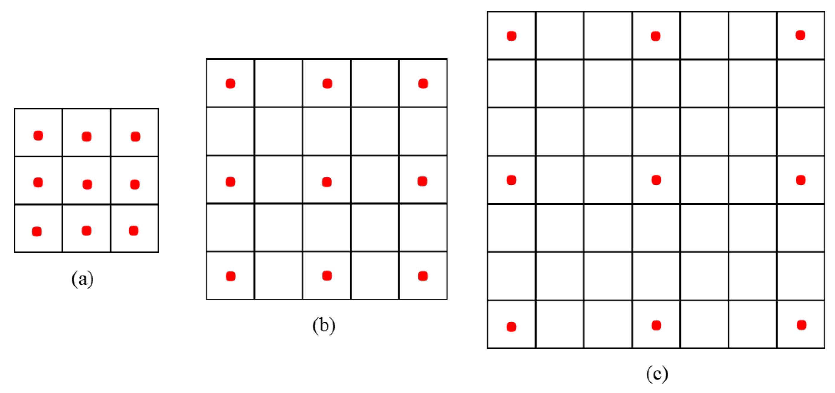
2.1. Dilated Convolution
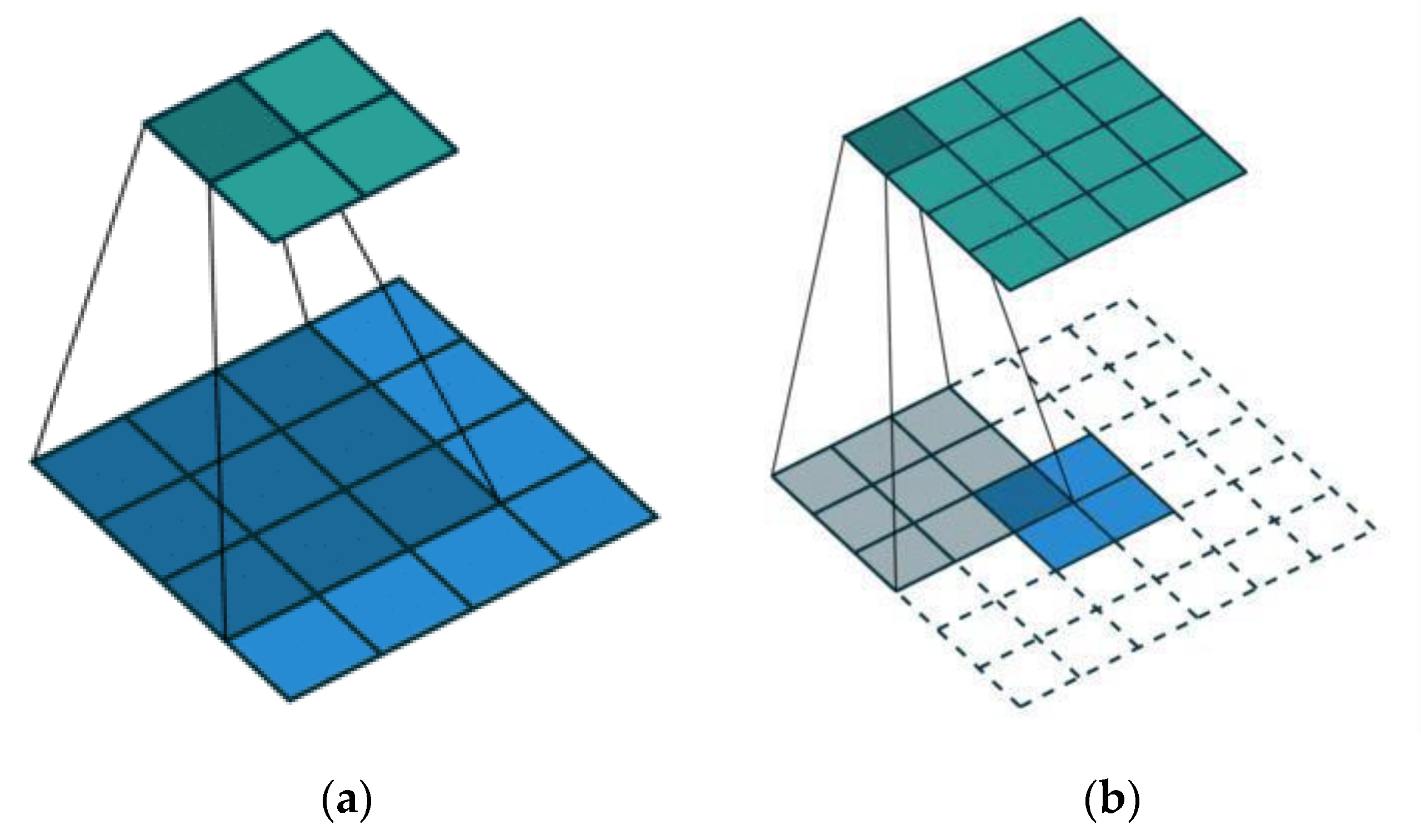
2.2. Transposed Convolution
2.3. Feature Fusion Methods
2.4. Skip Connection
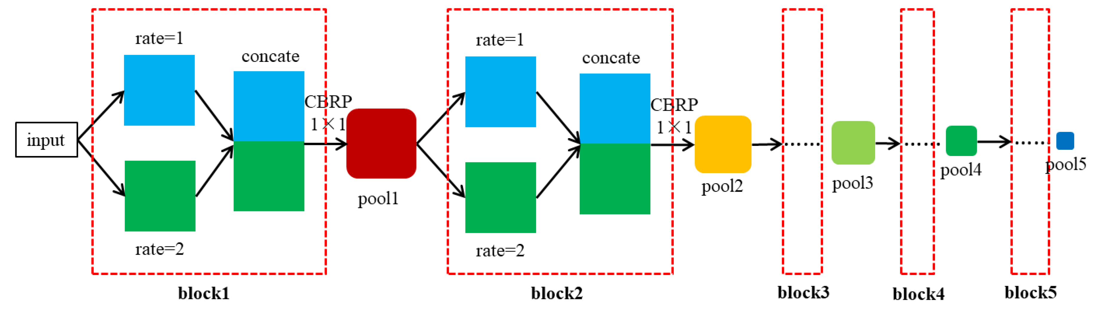
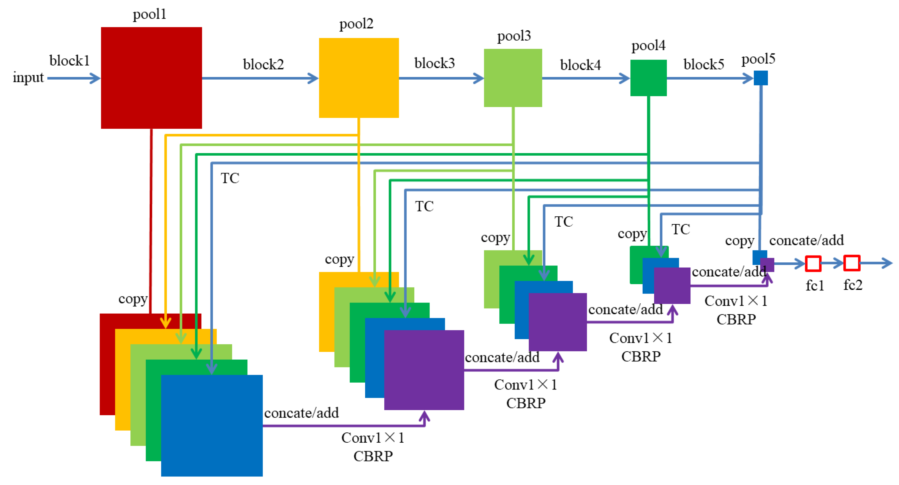
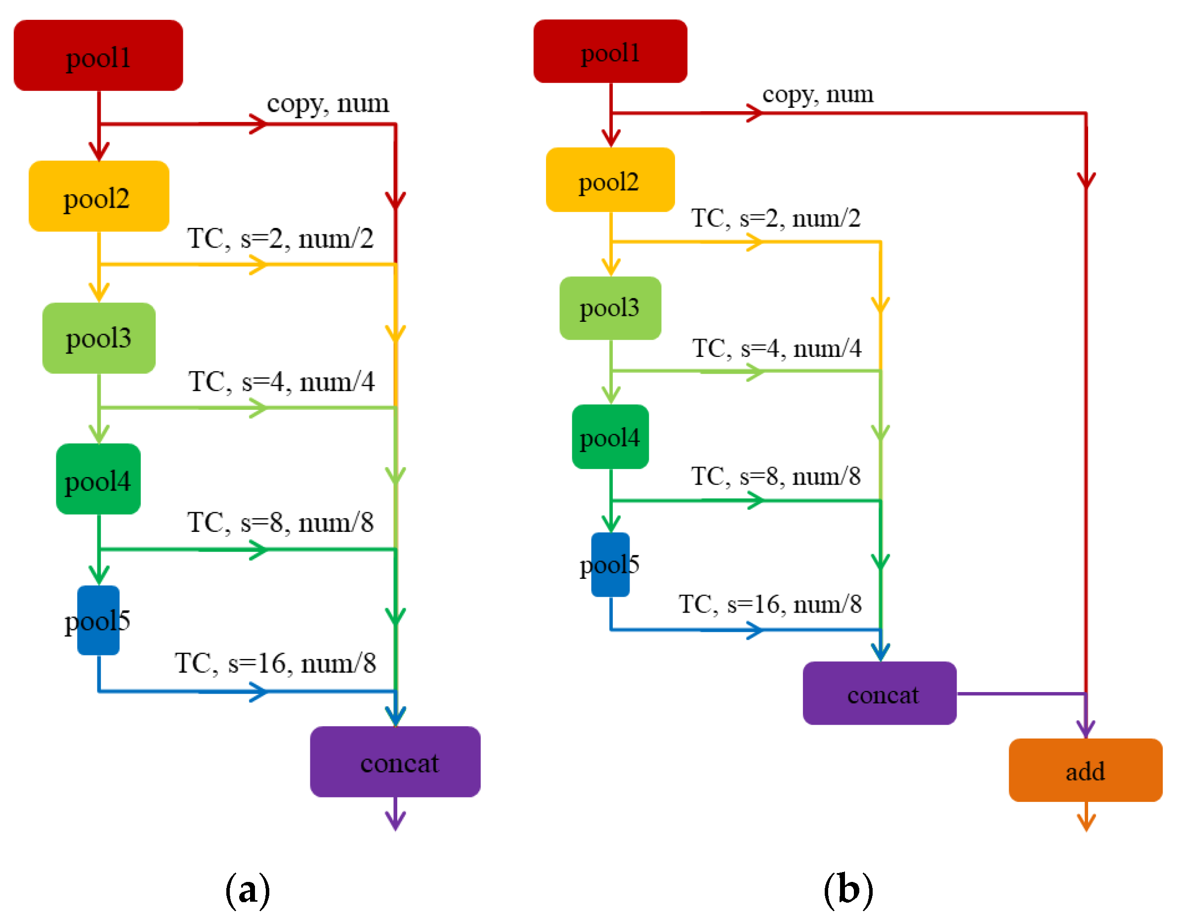
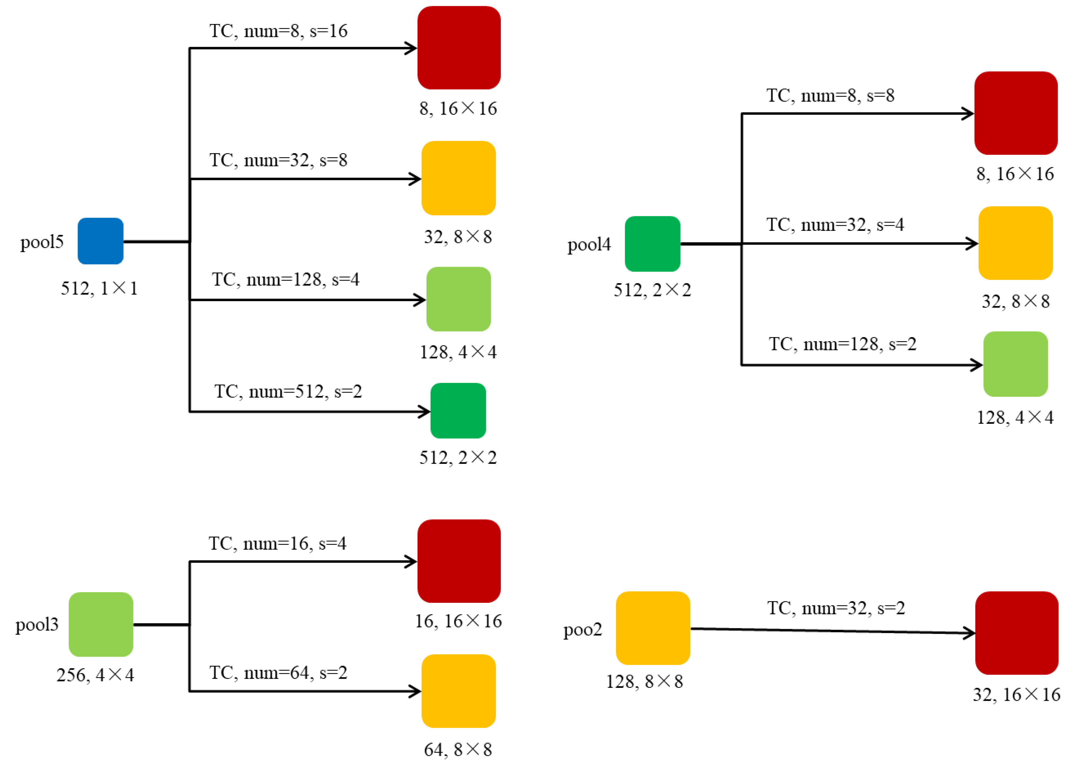
3. Fuse Different Features of CDTNet
4. Experiments
4.1. Datasets
4.2. Parameter Settings
4.3. Results and Discussion
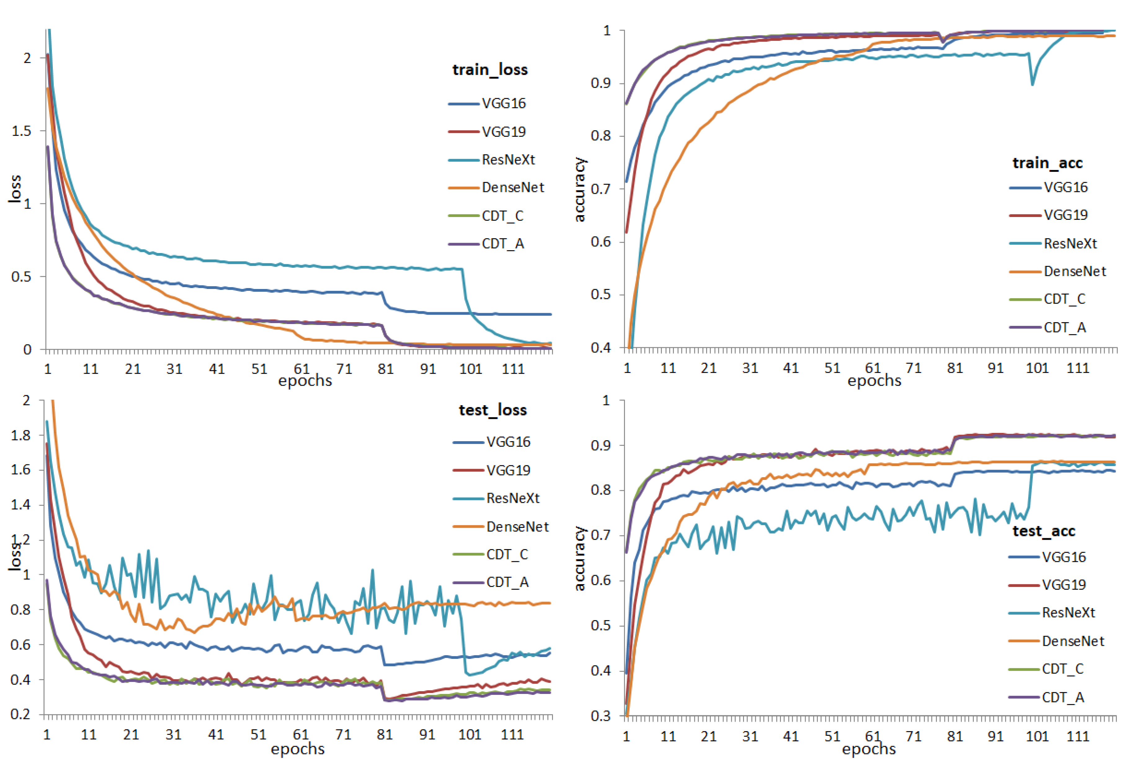
4.3.1. CIFAR-10
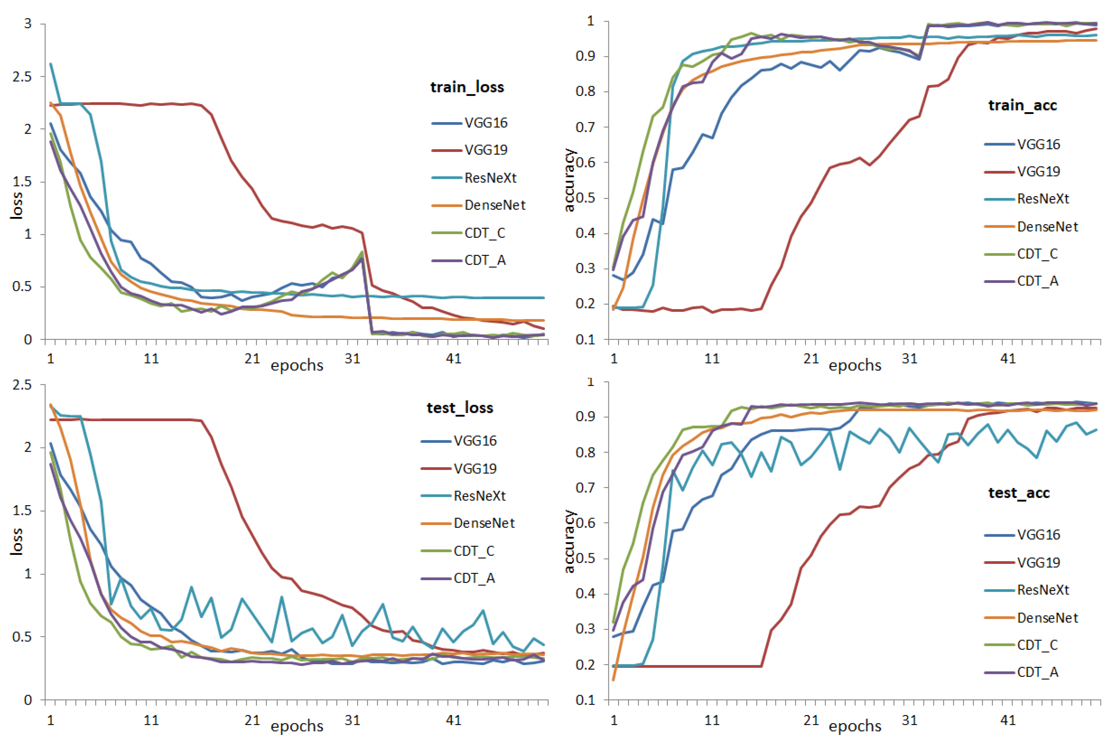
4.3.2. SVHN
4.3.3. FMNIST
4.3.4. Parameter of Models
5. Conclusions
Author Contributions
Funding
Informed Consent Statement
Conflicts of Interest
Abbreviations
References
- Lecun, Y.; Bottou, L.; Bengio, Y.; Haffner, P. Gradient-based learning applied to document recognition. Proc. IEEE 1998, 86, 2278–2324. [Google Scholar] [CrossRef]
- Krizhevsky, A.; Sutskever, I.; Hinton, G.E. Imagenet classification with deep convolutional neural networks. In Proceedings of the Advances in Neural Information Processing Systems, Carson, NV, USA, 3–6 December 2012; Volume 25, pp. 1097–1105. [Google Scholar]
- Simonyan, K.; Zisserman, A. Very deep convolutional networks for large-scale image recognition. arXiv 2014, arXiv:1409.1556. [Google Scholar]
- Szegedy, C.; Liu, W.; Jia, Y.; Sermanet, P.; Reed, S.; Anguelov, D.; Erhan, D.; Vanhoucke, V.; Rabinovich, A. Going deeper with convolutions. In Proceedings of the IEEE Conference on Computer Vision and Pattern Recognition (CVPR), Boston, MA, USA, 7–12 June 2015; pp. 1–9. [Google Scholar]
- Zhang, J.; Yu, J.; Tao, D. Local Deep-Feature Alignment for Unsupervised Dimension Reduction. IEEE Trans. Image Process. 2018, 27, 2420–2432. [Google Scholar] [CrossRef] [PubMed]
- Ren, S.; He, K.; Girshick, R.; Sun, J. Faster R-CNN: Towards Real-Time Object Detection with Region Proposal Networks. IEEE Trans. Pattern Anal. Mach. Intell. 2017, 39, 1137–1149. [Google Scholar] [CrossRef] [PubMed]
- Kim, Y. Convolutional Neural Networks for Sentence Classification. In Proceedings of the 2014 Conference on Empirical Methods in Natural Language Processing (EMNLP 2014), Doha, Qatar, 25–29 October 2014; pp. 1746–1751. [Google Scholar]
- Lin, T.Y.; Dollár, P.; Girshick, R.; He, K.; Hariharan, B.; Belongie, S. Feature pyramid networks for object detection. In Proceedings of the IEEE Conference on Computer Vision and Pattern Recognition, Honolulu, HI, USA, 21–26 July 2017; pp. 2117–2125. [Google Scholar]
- Huang, G.; Liu, Z.; Van Der Maaten, L.; Weinberger, K.Q. Densely connected convolutional networks. In Proceedings of the IEEE Conference on Computer Vision and Pattern Recognition, Honolulu, HI, USA, 21–26 July 2017; pp. 4700–4708. [Google Scholar]
- Tian, Z.; Shen, C.; Chen, H.; He, T. FCOS: Fully Convolutional One-Stage Object Detection. In Proceedings of the IEEE/CVF International Conference on Computer Vision (ICCV), Seoul, Korea, 27–28 October 2019; pp. 9626–9635. [Google Scholar] [CrossRef]
- Yilmazer, R.; Birant, D. Shelf Auditing Based on Image Classification Using Semi-Supervised Deep Learning to Increase On-Shelf Availability in Grocery Stores. Sensors 2021, 21, 327. [Google Scholar] [CrossRef]
- Zeng, J.; Zhang, D.; Li, Z.; Li, X. Semi-Supervised Training of Transformer and Causal Dilated Convolution Network with Applications to Speech Topic Classification. Appl. Sci. 2021, 11, 5712. [Google Scholar] [CrossRef]
- Lessmann, N.; Van Ginneken, B.; Zreik, M.; De Jong, P.A.; De Vos, B.D.; Viergever, M.A.; Isgum, I. Automatic Calcium Scoring in Low-Dose Chest CT Using Deep Neural Networks with Dilated Convolutions. IEEE Trans. Med. Imaging 2018, 37, 615–625. [Google Scholar] [CrossRef]
- Xia, H.; Sun, W.; Song, S.; Mou, X. Md-Net: Multi-scale Dilated Convolution Network for CT Images Segmentation. Neural Process. Lett. 2020, 51, 2915–2927. [Google Scholar] [CrossRef]
- Wang, T.; Sun, M.; Hu, K. Dilated Deep Residual Network for Image Denoising. In Proceedings of the IEEE 29th International Conference on Tools with Artificial Intelligence (ICTAI), Boston, MA, USA, 6–8 November 2017; pp. 1272–1279. [Google Scholar]
- Tian, C.; Xu, Y.; Li, Z.; Zuo, W.; Fei, L.; Liu, H. Attention-guided CNN for image denoising. Neural Netw. 2020, 124, 117–129. [Google Scholar] [CrossRef]
- Peng, Y.; Zhang, L.; Liu, S.; Wu, X.; Zhang, Y.; Wang, X. Dilated Residual Networks with Symmetric Skip Connection for image denoising. Neurocomputing 2019, 345, 67–76. [Google Scholar] [CrossRef]
- Shelhamer, E.; Long, J.; Darrell, T. Fully Convolutional Networks for Semantic Segmentation. IEEE Trans. Pattern Anal. Mach. Intell. 2017, 39, 640–651. [Google Scholar] [CrossRef] [PubMed]
- Peng, C.; Zhang, X.; Yu, G.; Luo, G.; Sun, J. Large Kernel Matters-Improve Semantic Segmentation by Global Convolutional Network. In Proceedings of the 2017 IEEE Conference on Computer Vision and Pattern Recognition (CVPR), Honolulu, HI, USA, 21–26 July 2017; pp. 1743–1751. [Google Scholar]
- Chen, L.; Papandreou, G.; Kokkinos, I.; Murphy, K.; Yuille, A.L. DeepLab: Semantic Image Segmentation with Deep Convolutional Nets, Atrous Convolution, and Fully Connected CRFs. IEEE Trans. Pattern Anal. Mach. Intell. 2018, 40, 834–848. [Google Scholar] [CrossRef] [PubMed]
- Zhou, Y.; Chang, H.; Lu, Y.; Lu, X.; Zhou, R. Improving the Performance of VGG Through Different Granularity Feature Combinations. IEEE Access 2021, 9, 26208–26220. [Google Scholar] [CrossRef]
- Dong, L.J.; Yi, W.X.; Yi, C.; Peng, Y.H. Structure optimization of convolutional neural networks: A survey. Acta Autom. Sin. 2020, 46, 24–37. [Google Scholar] [CrossRef]
- Li, Y.; Yin, G.; Zhuang, W.; Zhang, N.; Wang, J.; Geng, K. Compensating Delays and Noises in Motion Control of Autonomous Electric Vehicles by Using Deep Learning and Unscented Kalman Predictor. IEEE Trans. Syst. Man Cybern. 2020, 50, 4326–4338. [Google Scholar] [CrossRef]
- Wang, Q.; Huang, W.; Xiong, Z.; Li, X. Looking Closer at the Scene: Multiscale Representation Learning for Remote Sensing Image Scene Classification. IEEE Trans. Neural Netw. Learn. Syst. 2020, 33, 1414–1428. [Google Scholar] [CrossRef]
- He, K.; Zhang, X.; Ren, S.; Sun, J. Deep residual learning for image recognition. In Proceedings of the IEEE Conference on Computer Vision and Pattern Recognition (CVPR), Las Vegas, NV, USA, 27–30 June 2016; pp. 770–778. [Google Scholar] [CrossRef]
- Szegedy, C.; Vanhoucke, V.; Ioffe, S.; Shlens, J.; Wojna, Z. Rethinking the Inception Architecture for Computer Vision. In Proceedings of the IEEE Conference on Computer Vision and Pattern Recognition (CVPR), Las Vegas, NV, USA, 27–30 June 2016; pp. 2818–2826. [Google Scholar] [CrossRef]
- Wang, R.; Gong, M.; Tao, D. Receptive Field Size Versus Model Depth for Single Image Super-Resolution. IEEE Trans. Image Process. 2020, 29, 1669–1682. [Google Scholar] [CrossRef]
- Li, H.; Qi, F.; Shi, G.; Lin, C. A multiscale dilated dense convolutional network for saliency prediction with instance-level attention competition. J. Vis. Commun. Image Represent. 2019, 64, 102611. [Google Scholar] [CrossRef]
- Luo, W.; Li, Y.; Urtasun, R.; Zemel, R. Understanding the effective receptive field in deep convolutional neural networks. In Proceedings of the 30th International Conference on Neural Information Processing Systems, Barcelona, Spain, 5–10 December 2016; pp. 4898–4906. [Google Scholar]
- Huang, G.; Liu, S.; Maaten, L.V.D.; Weinberger, K.Q. CondenseNet: An efficient DenseNet using learned group convolutions. In Proceedings of the 2018 IEEE/CVF Conference on Computer Vision and Pattern Recognition, Salt Lake City, UT, USA, 18–23 June 2018; pp. 2752–2761. [Google Scholar] [CrossRef]
- Liu, Z.; Sun, M.; Zhou, T.; Huang, G.; Darrell, T. Rethinking the value of network pruning. arXiv 2018, arXiv:1810.05270. [Google Scholar]
- Zheng, Q.; Tian, X.; Yang, M. PAC-Bayesian framework based drop-path method for 2D discriminative convolutional network pruning. Multidim Syst. Sign Process. 2020, 31, 793–827. [Google Scholar] [CrossRef]
- Kendall, A.; Gal, Y. What uncertainties do we need in bayesian deep learning for computer vision? In Proceedings of the Advances in Neural Information Processing Systems (NIPS), Long Beach, CA, USA, 4–9 December 2017; pp. 5574–5584. [Google Scholar]
- Hinton, G.E.; Srivastava, N.; Krizhevsky, A.; Sutskever, I.; Salakhutdinov, R.R. Improving neural networks by preventing co-adaptation of feature detectors. Comput. Sci. 2012, 3, 212–223. [Google Scholar]
- Zheng, Q.; Zhao, P.; Li, Y. Spectrum interference-based two-level data augmentation method in deep learning for automatic modulation classification. Neural Comput. Appl. 2021, 33, 7723–7745. [Google Scholar] [CrossRef]
- Larsson, G.; Maire, M.; Shakhnarovich, G. Fractalnet: Ultra-deep neural networks without residuals. arXiv 2016, arXiv:1605.07648. [Google Scholar]
- Zheng, Q.; Tian, X.; Yang, M.; Wang, H. Differential learning: A powerful tool for interactive content-based image retrieval. Eng. Lett. 2019, 27, 202–215. [Google Scholar]
- Kobayashi, T. Flip-invariant motion representation. In Proceedings of the Proceedings of the IEEE International Conference on Computer Vision (ICCV), Venice, Italy, 22–29 October 2017; pp. 5628–5637. [Google Scholar]
- Zheng, Q.; Yang, M.; Tian, X.; Jiang, N.; Wang, D. A full stage data augmentation method in deep convolutional neural network for natural image classification. Discret. Dyn. Nat. Soc. 2020, 2020, 4706576. [Google Scholar] [CrossRef]
- He, Y.; Keuper, M.; Schiele, B.; Fritz, M. Learning Dilation Factors for Semantic Segmentation of Street Scenes. In German Conference on Pattern Recognition; Roth, V., Vetter, T., Eds.; Springer: Berlin/Heidelberg, Germany, 2017; pp. 41–51. [Google Scholar] [CrossRef]
- Qu, J.; Su, C.; Zhang, Z.; Razi, A. Dilated Convolution and Feature Fusion SSD Network for Small Object Detection in Remote Sensing Images. IEEE Access 2020, 8, 82832–82843. [Google Scholar] [CrossRef]
- Heo, W.-H.; Kim, H.; Kwon, O.-W. Source Separation Using Dilated Time-Frequency DenseNet for Music Identification in Broadcast Contents. Appl. Sci. 2020, 10, 1727. [Google Scholar] [CrossRef]
- Heo, W.-H.; Kim, H.; Kwon, O.-W. Integrating Dilated Convolution into DenseLSTM for Audio Source Separation. Appl. Sci. 2021, 11, 789. [Google Scholar] [CrossRef]
- Ronneberger, O.; Fischer, P.; Brox, T. Invited Talk: U-Net: Convolutional Networks for Biomedical Image Segmentation. In Bildverarbeitung für die Medizin; Fritzsche, K., Deserno, G., Lehmann, T., Handels, H., Tolxdorff, T., Eds.; Springer: Berlin, Germany, 2017. [Google Scholar] [CrossRef]
- Zeiler, M.D.; Taylor, G.W.; Fergus, R. Adaptive deconvolutional networks for mid and high level feature learning. In Proceedings of the 2011 International Conference on Computer Vision, Barcelona, Spain, 6–13 November 2011; pp. 2018–2025. [Google Scholar] [CrossRef]
- Xie, S.; Girshick, R.; Dollar, P.; Tu, Z.; He, K. Aggregated Residual Transformations for Deep Neural Networks. In Proceedings of the 2017 IEEE Conference on Computer Vision and Pattern Recognition (CVPR), Honolulu, HI, USA, 21–26 July 2017; pp. 5987–5995. [Google Scholar] [CrossRef]
- Yu, F.; Koltun, V. Multi-scale context aggregation by dilated convolutions. arXiv 2016, arXiv:1511.07122. [Google Scholar]
- Wang, F.; Zhu, H.; Li, W.; Li, K. A hybrid convolution network for serial number recognition on banknotes. Inf. Sci. 2020, 512, 952–963. [Google Scholar] [CrossRef]
- Lu, Z.; Bai, Y.; Chen, Y. The classification of gliomas based on a Pyramid dilated convolution resnet model. Pattern Recognit. Lett. 2020, 133, 173–179. [Google Scholar] [CrossRef]
- Yao, S.; Chen, Y.; Tian, X.; Jiang, R.; Ma, S. An Improved Algorithm for Detecting Pneumonia Based on YOLOv3. Appl. Sci. 2020, 10, 1818. [Google Scholar] [CrossRef]
- Lian, X.; Pang, Y.; Han, J.; Pan, J. Cascaded hierarchical atrous spatial pyramid pooling module for semantic segmentation. Pattern Recognit. 2021, 110, 107622. [Google Scholar] [CrossRef]
- Zeiler, M.D.; Krishnan, D.; Taylor, G.W.; Fergus, R. Deconvolutional networks. In Proceedings of the IEEE Computer Society Conference on Computer Vision and Pattern Recognition, San Francisco, CA, USA, 13–18 June 2010; pp. 2528–2535. [Google Scholar] [CrossRef]
- Gulrajani, I.; Kumar, K.; Ahmed, F.; Taiga, A.A.; Visin, F.; Vazquez, D.; Courville, A. Pixelvae: A latent variable model for natural images. arXiv 2016, arXiv:1611.05013. [Google Scholar]
- Pu, Y.; Yuan, W.; Stevens, A.; Li, C.; Carin, L. A deep generative deconvolutional image model. Artif. Intell. Stat. 2016, 51, 741–750. [Google Scholar]
- Dumoulin, V.; Visin, F. A guide to convolution arithmetic for deep learning. arXiv 2016, arXiv:1603.07285. [Google Scholar]
- Yang, J.; Zhang, T.; Song, W.; Song, C. Fuzzy license plate restoration method based on convolution and transposed convolution. Sci. Technol. Eng. 2018, 18, 241–249. [Google Scholar]
- Bukka, S.R.; Gupta, R.; Magee, A.R. Assessment of unsteady flow predictions using hybrid deep learning based reduced order models. arXiv 2020, arXiv:2009.04396. [Google Scholar] [CrossRef]
- Fu, J.; Liu, J.; Li, Y. Contextual Deconvolution Network for Semantic Segmentation. Pattern Recognit. 2020, 101, 107152. [Google Scholar] [CrossRef]
- Noh, H.; Hong, S.; Han, B. Learning deconvolution network for semantic segmentation. In Proceedings of the 2015 IEEE International Conference on Computer Vision (ICCV), Santiago, Chile, 7–13 December 2015; pp. 1520–1528. [Google Scholar]
- Cui, Z.; Chang, H.; Shan, S.; Zhong, B.; Chen, X. Deep network cascade for image super-resolution. In Proceedings of the European Conference on Computer Vision, Zurich, Switzerland, 6–12 September 2014; pp. 49–64. [Google Scholar]
- Lin, G.; Wu, Q.; Qiu, L.; Huang, X. Image super-resolution using a dilated convolutional neural network. Neurocomputing 2018, 275, 1219–1230. [Google Scholar] [CrossRef]
- Li, W.; Li, B.; Yuan, C.; Li, Y.; Wu, H.; Hu, W.; Wang, F. Anisotropic Convolution for Image Classification. IEEE Trans. Image Process. 2020, 29, 5584–5595. [Google Scholar] [CrossRef] [PubMed]
- Fu, J.; Liu, J.; Wang, Y. Stacked deconvolutional network for semantic segmentation. IEEE Trans. Image Process. 2019, 1–13. [Google Scholar] [CrossRef] [PubMed]
- Mozaffari, M.H.; Lee, W.-S. Bownet: Dilated convolution neural network for ultrasound tongue contour extraction. J. Acoust. Soc. Am. 2019, 146, 2940–2941. [Google Scholar] [CrossRef]
- Chen, H.; Sun, K.; Tian, Z. BlendMask: Top-Down Meets Bottom-Up for Instance Segmentation. In Proceedings of the IEEE Conference on Computer Vision and Pattern Recognition, Seattle, WA, USA, 13–19 June 2020; pp. 8573–8581. [Google Scholar]
- Hu, J.; Shen, L.; Albanie, S.; Sun, G.; Wu, E. Squeeze-and-Excitation Networks. IEEE Trans. Pattern Anal. Mach. Intell. 2020, 42, 2011–2023. [Google Scholar] [CrossRef] [PubMed]
- Zhang, Z.; Wang, X.; Jung, C. DCSR: Dilated Convolutions for Single Image Super-Resolution. IEEE Trans. Image Process. 2019, 28, 1625–1635. [Google Scholar] [CrossRef]
- Dai, Y.; Zhuang, P. Compressed sensing MRI via a multi-scale dilated residual convolution network. Magn. Reson. Imaging 2019, 63, 93–104. [Google Scholar] [CrossRef]
- Yu, F.; Wang, D.; Shelhamer, E.; Darrell, T. Deep Layer Aggregation. In Proceedings of the 2018 IEEE/CVF Conference on Computer Vision and Pattern Recognition, Salt Lake City, UT, USA, 18–23 June 2018; pp. 2403–2412. [Google Scholar] [CrossRef]
- Ioffe, S.; Szegedy, C. Batch normalization: Accelerating deep network training by reducing internal covariate shift. In Proceedings of the 32nd International Conference on Machine Learning, Lille, France, 7–9 July 2015; pp. 448–456. [Google Scholar]
- Nair, V.; Hinton, G. Rectified linear units improve restricted Boltzmann machines. In Proceedings of the 27th International Conference on International Conference on Machine Learning, Haifa, Israel, 21–24 June 2010; pp. 807–814. [Google Scholar]
- Krizhevsky, A.; Hinton, G. Learning Multiple Layers of Features from Tiny Images; Technical Report; University of Toronto: Toronto, ON, Canada, 2009. [Google Scholar]
- Netzer, Y.; Wang, T.; Coates, A.; Bissacco, A.; Wu, B.; Ng, A.Y. Reading digits in natural images with unsupervised feature learning. In Proceedings of the Conference on Neural Information Processing Systems (NIPS), Granada, Spain, 12–15 December 2011; pp. 1–9. [Google Scholar]
- Xiao, H.; Rasul, K.; Vollgraf, R. Fashion-MNIST: A Novel Image Dataset for Benchmarking Machine Learning Algorithms. arXiv 2017, arXiv:1708.07747. [Google Scholar]
- Shafiq, S.; Azim, T. Introspective analysis of convolutional neural networks for improving discrimination performance and feature visualisation. PeerJ Comput. Sci. 2021, 7, e497. [Google Scholar] [CrossRef]
- Li, X.; Li, F.; Fern, X.; Raich, R. Filter shaping for convolutional neural networks. In Proceedings of the ICLR 2017 Conference, Toulon, France, 24–26 April 2017. [Google Scholar]


| Model | Baseline | Training Loss | Training Accuracy | Test Loss | Test Accuracy |
|---|---|---|---|---|---|
| CDT_C | VGG16 | 55.3% ↓ | 3.99% ↑ | 36.76% ↓ | 9.43% ↑ |
| CDT_C | VGG19 | 20.3% ↓ | 2.42% ↑ | 14.1% ↓ | 1.48% ↑ |
| CDT_C | ResNeXt | 67.17% ↓ | 6.84% ↑ | 54.36% ↓ | 19.92% ↑ |
| CDT_C | DenseNet | 28.4% ↓ | 7.61% ↑ | 56% ↓ | 8.89% ↑ |
| CDT_A | VGG16 | 55.15% ↓ | 3.96% ↑ | 37.57% ↓ | 9.61% ↑ |
| CDT_A | VGG19 | 20.05% ↓ | 2.39% ↑ | 15.19% ↓ | 1.65% ↑ |
| CDT_A | ResNeXt | 67.06% ↓ | 6.81% ↑ | 54.94% ↓ | 20.13% ↑ |
| CDT_A | DenseNet | 28.16% ↓ | 7.58% ↑ | 56.6% ↓ | 9.07% ↑ |
| Model | Baseline | Training Loss | Training Accuracy | Test Loss | Test Accuracy |
|---|---|---|---|---|---|
| CDT_C | VGG16 | 25.55% ↓ | 9.83% ↑ | 18.14% ↓ | 9.13% ↑ |
| CDT_C | VGG19 | 68.83% ↓ | 58.73% ↑ | 62.85% ↓ | 54.81% ↑ |
| CDT_C | ResNeXt | 42.16% ↓ | 5.54% ↑ | 40.8% ↓ | 17.49% ↑ |
| CDT_C | DenseNet | 13.84% ↓ | 5.92% ↑ | 17.68% ↓ | 3.82% ↑ |
| CDT_A | VGG16 | 23.3% ↓ | 7.71% ↑ | 15.98% ↓ | 6.79% ↑ |
| CDT_A | VGG19 | 67.89% ↓ | 55.67% ↑ | 61.87% ↓ | 51.48% ↑ |
| CDT_A | ResNeXt | 40.41% ↓ | 3.50% ↑ | 39.24% ↓ | 14.97% ↑ |
| CDT_A | DenseNet | 11.24% ↓ | 3.87% ↑ | 15.51% ↓ | 1.59% ↑ |
| Models | VGG16 | VGG19 | ResNeXt | DenseNet | CDT_C | CDT_A |
|---|---|---|---|---|---|---|
| Accuracy | 0.9213 | 0.9207 | 0.9172 | 0.9133 | 0.9337 | 0.9331 |
Publisher’s Note: MDPI stays neutral with regard to jurisdictional claims in published maps and institutional affiliations. |
© 2022 by the authors. Licensee MDPI, Basel, Switzerland. This article is an open access article distributed under the terms and conditions of the Creative Commons Attribution (CC BY) license (https://creativecommons.org/licenses/by/4.0/).
Share and Cite
Zhou, Y.; Chang, H.; Lu, Y.; Lu, X. CDTNet: Improved Image Classification Method Using Standard, Dilated and Transposed Convolutions. Appl. Sci. 2022, 12, 5984. https://doi.org/10.3390/app12125984
Zhou Y, Chang H, Lu Y, Lu X. CDTNet: Improved Image Classification Method Using Standard, Dilated and Transposed Convolutions. Applied Sciences. 2022; 12(12):5984. https://doi.org/10.3390/app12125984
Chicago/Turabian StyleZhou, Yuepeng, Huiyou Chang, Yonghe Lu, and Xili Lu. 2022. "CDTNet: Improved Image Classification Method Using Standard, Dilated and Transposed Convolutions" Applied Sciences 12, no. 12: 5984. https://doi.org/10.3390/app12125984