The Relationship between Process Capability and Quality of Measurement System

Abstract

This article deals with the design of appropriate measures that had to be taken for the implemented measurement system. The measurement result was significantly negatively affected by several factors. Forty-five samples of shafts used in the production of surgical drills were measured. Measurements were performed by metrological appraisers with a calibrated digital micrometer. Measurement and subsequent data processing revealed low process capability (CP and PP indices). A large portion of the shafts had an observed size below the lower specific limit (LSL). Therefore, it was necessary to take corrective action. This paper focuses on the corrective measures implemented in the measurement system. The micrometer met the requirements of the standard and was metrologically capable. The shafts were measured by eight metrological appraisers, so attention was focused on the potential impact of the metrological appraiser. The measured data were evaluated by uncertainty analysis, paired t-tests, measurement systems analysis (MSA) and Cohen’s kappa. The number of non-compliant shafts was shown to increase with decreasing measurement capability. The measurement system was evaluated as conditionally capable, even incapable. One possibility was to identify the optimal pair of metrological appraisers. The pair of metrological appraisers E and F appeared to be the most suitable combination for most methods. Due to the relatively high %EV index, the second option was to improve the work with the measuring instrument, that is, improve the training and supervision of metrological appraisers in the measurement process. Repeated measurements by the pair with the highest capability (metrological appraisers E and F) resulted in an increase in the value of the capability indices and a decrease in the number of shafts out of tolerance for the same shafts. As the value of these indices was lower than 1.33 during repeated measurements, corrective measures had to be taken, not only in the measurement system, but also in the production system.

1. Introduction

After setting up the CNC machine (lathe), a trial production of shafts (for surgical drills) was started. Dimension d₂ was measured by metrological appraiser A on the first 45 products. Each measurement was repeated three times. A digital screw micrometer Kinex with resolution d* = 0.001 mm was used as the measurement equipment.

The measured values were compared with the value specifically required by the customer. This represented the target value T = 7.98 mm, LSL = 7.958 mm and USL = 7.98 mm. The calculated values of descriptive statistics (arithmetic mean, standard deviation, test for outliers and normality) and process capability indices are given in

Table 1. Descriptive statistics, capability indices and numbers of noncompliant shafts.

Metrological Appraiser	A	B	C	D	E	F	G	H
$\overline{x}$ (mean)	7.9577	7.9593	7.9547	7.9552	7.9571	7.9575	7.9575	7.9579
SD	0.0062	0.0061	0.0056	0.0065	0.0061	0.0062	0.0095	0.0050
Max	7.9740	7.9750	7.9713	7.9720	7.9723	7.97267	7.9850	7.9710
Min	7.9417	7.9473	7.9430	7.9420	7.9450	7.9447	7.9417	7.9477
Distribution	N	N	N	N	N	N	N	N
p-value of distribution test	0.5498	0.6979	0.4096	0.6918	0.6491	0.4269	0.4739	0.2153
Outliers	0	0	0	0	0	0	0	0
Capability Statistics
CP	0.8834	0.9855	0.8478	0.8584	0.8136	0.9397	0.4531	1.0519
CPL	−0.0214	0.1188	−0.2546	−0.2156	−0.0641	−0.0386	−0.0204	−0.0064
CPU	1.7883	1.8522	1.9501	1.9325	1.6914	1.9120	0.9266	2.1102
CPK	−0.0214	0.1188	−0.2546	−0.2156	−0.0641	−0.0386	−0.0204	−0.0064
PP	0.5958	0.6034	0.6550	0.5602	0.6002	0.5949	0.3841	0.7297
PPL	−0.0144	0.0727	−0.1967	−0.1407	−0.0473	−0.0244	−0.0173	−0.0044
PPU	1.2061	1.1341	1.5067	1.2610	1.2477	1.2142	0.7856	1.4638
PPK	−0.0144	0.0727	−0.1967	−0.1407	−0.0473	−0.0244	−0.0173	−0.0044
Parts Per Million
ppm < LSL	555,556	400,000	800,000	688,889	600,000	577,778	600,000	600,000
ppm > USL	0	0	0	0	0	0	22222	0
ppm Total	555,556	400,000	800,000	688,889	600,000	577,778	622,222	600,000
Short-Term Defects
ppm < LSL	525,614	360,784	777,517	741,134	576,252	546,094	524,450	507,630
ppm > USL	0.0405	0.0138	0.0025	0.0034	0.1946	0.0044	2719.97	0.0001
ppm Total	525,614	360,784	777,517	741,134	576,252	546,094	527,170	507,630
Overall or Long-Term Defects
ppm < LSL	517,282	413,638	722,458	663,525	556,407	529,220	520,732	505,293
ppm > USL	148.305	334.268	3.0899	77.4525	90.8837	134.940	9220.48	5.6315
ppm Total	517,430	413,972	72,246	663,602	556,498	529,355	529,952	505,298

. The presented calculation assumed that the investigated parameter (shaft diameter) followed the normal distribution.

Quantum XL software (Quantum XL 2016 v5.60, Orlando, FL, USA) was used for the calculation. The results are shown in Table 1. Outliers were determined by the Grubbs’ test (at the selected significance level α = 0.05) using GraphPad software (https://www.graphpad.com/quickcalcs/index.cfm, accessed on 26 January 2021). The test confirmed that the measurement was subject to gross errors and was not under statistical control. The Anderson–Darling test was used to test for normality. If the value in Table 1 was p > 0.05, the analyzed file had a normal distribution.

The most common explanation of the C_P and P_P indices is this: C_P is the short-term capability of a process, and P_P is its long-term capability. The truth is that these statistical indices are much more than that, and it is important to understand what the process and capability statistics really mean. However, in order to reveal the true state of the process, obtained data must be accurately assessed and interpreted (B).

Process capability studies are conducted for three reasons:

• To assess the potential capability of a process at a specific point or points in time in order to obtain values within a specification;
• To predict the future potential of a process in order to create a value within specifications with the use of meaningful metrics;
• To identify improvement opportunities in the process by reducing or possibly eliminating sources of variability [1].

C_P and C_PK are considered short-term potential capability metrics for a process. P_P is a process index that numerically describes the long-term capability of a process assuming that it was analyzed and stayed in control. It is a simple and straightforward indicator of process performance. It is used when a process is initially starting out [2].

The long-term examination of process capability serves to determine the qualitative capability of the process under real production conditions. It is performed over a longer period (e.g., 20 production days of series production) to take into account all significant effects causing process variability.

C_PL or P_PL are measures of the potential capability of the process based on its lower specification limit. They are ratios that compare two values: the distance from the process mean to the lower specification limit (LSL) and the one-sided spread of the process (the 3-σ variation) based on the within-subgroup standard deviation. C_PU or P_PU are measures of the potential capability of a process based on its upper specification limit. C_PU is a ratio that compares two values: the distance from the process mean to the upper specification limit (USL) and one-sided spread of the process (the 3-σ variation) based on the variation within the subgroups. Because it considers both the process mean and the process spread, it evaluates both the location and variation (within subgroups) of the process [3].

After evaluating the data measured by metrological appraiser A, it was found that all 45 shafts met the USL tolerance requirement. On the other hand, up to 57.78% of shafts had a diameter smaller than LSL. As can be seen from Table 1, as a result, the C_P capability index was very low (0.8834), as was the C_PK index, which signaled a process deviation. This was also confirmed by the average value of the observed dimension (7.9588). It exceeded the LSL value by only 0.0003 mm. This would represent a failure rate of 550,000 ppm.

The same shafts have already been produced in the past. The nonconformities also occurred at that time, but not to such an extent. Customers complained about increased noise and disturbing sound effects. According to regulations [4,5], the upper permissible noise level of the drill is 90 dB. A noise level of 93.3 dB was measured for the drills complained about by the customer. The measurement was tentative, as an uncertified measuring instrument was used. In addition to the excessive noise, an unpleasant, disturbing noise also occurred. The cause of these disturbing sound effects may have been the excessive clearance between the shaft and the bearing, allowing the shaft to vibrate.

Due to the large number of nonconforming products, production was stopped. It was necessary to analyze the causes of nonconforming product occurrence. Based on the analysis, effective corrective action had to be taken. A cause-and-effect diagram was used in the analysis to determine the causes and consequences (Figure 1). This diagram has been used by several authors, such as Girman et al. [6,7,8,9,10], as the basis of fault analysis. It allows for a “clarification” of the problem and is often used to identify the sources that contribute to the analyzed problem and the relationships between them [11,12,13,14].

As can be seen in Figure 1, the consequence—problem statement—is a high number of nonconforming (defective) shafts (high ppm of defective shafts). The categories were modified according to actual problems in the process of shaft production (Manpower, Materials, Methods, Measurement, Environment and Machine).

The category “Manpower” is extremely important because the factors involved also influence other categories. It mainly represents the appraiser of the CNC lathe (metrological appraiser is included in the Measurement category). Possible sub-causes are incompetence, setting error, inappropriate interventions into the CNC machine during production, no input and output control and noncompliance with regulations.

Two possible causes have been identified in the category “Materials”: inappropriate material or material swap (mismatch), either in terms of its composition or dimensions. This may be due to poor records or a poor measurement system.

Two possible causes were also identified in the category “Methods”: incorrect method of metrological traceability maintenance and incorrect use of the metrological procedure of the organization. It should be noted that the metrological order is confusing, difficult to understand and can lead to errors.

Regarding the category “Measurement”, three possible causes of nonconformity of the final product were identified, related to the measurement system and measurement process:

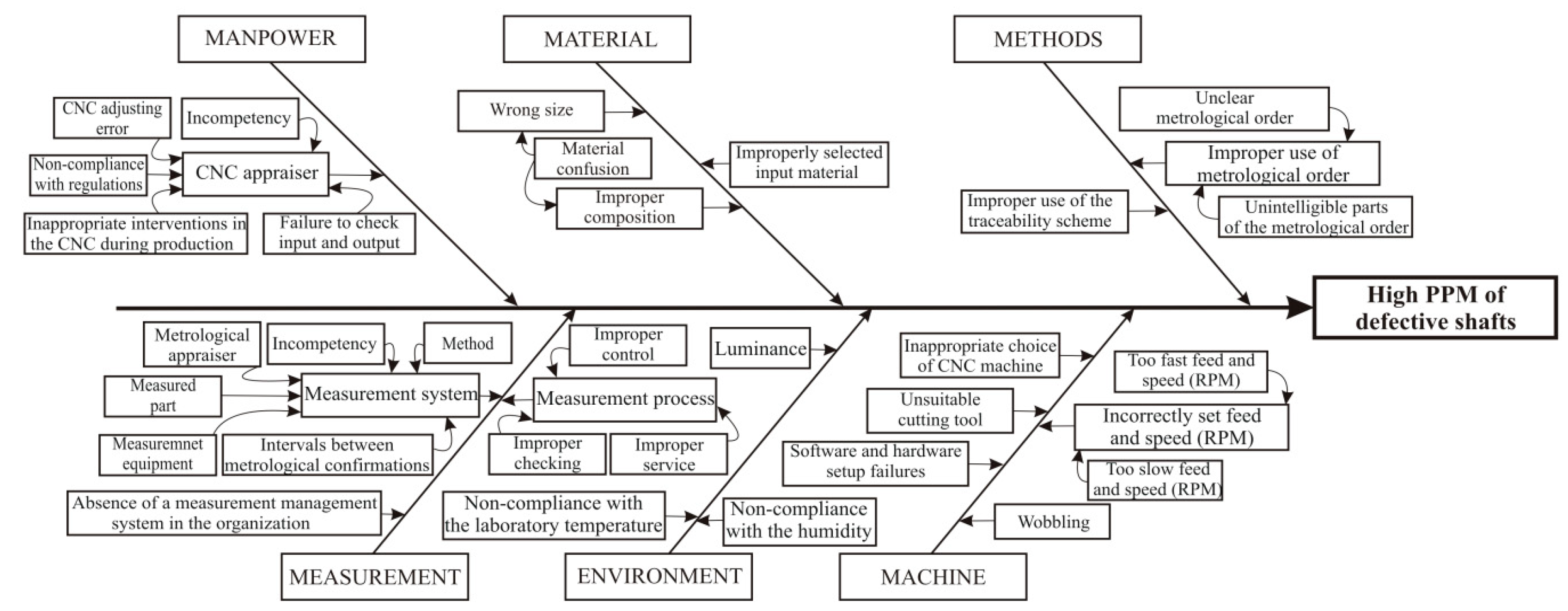
• The measurement system can be influenced by the measurement equipment, the measured part, the metrological appraiser, the measurement methods, the intervals between metrological confirmations and the environment;
• The measurement process is influenced by the way of its management, organizational and material support and control;
• The root cause for this rib is the absence of a measurement management system in the organization.

The category “Environment” has two possible causes: noncompliance with the laboratory temperature and noncompliance with the humidity. The location of the CNC lathe and the measuring place met the conditions for a class IV calibration laboratory in terms of temperature, humidity and lighting [15], i.e., temperature (20 ± 2) °C, relative humidity (20–60)%, sound level ≤ 70 dB and illuminance min. 800 lx.

Causes identified in the “Machine” category: improper machine selection, wobbling, improper feed setting (too fast), improper cutting tool (poor quality, poorly clamped, bad geometry), incorrectly selected cutting speed and software and hardware settings faults.

This research focused mainly on the “Measurement” category. Before addressing the causes specified in the other categories, it was necessary to make sure that the measured values were accurate, precise and true.

It is possible that metrological appraiser A performed the measurement process incorrectly. To check his results, a measurement system was used, where the dimension d₂ was measured on ten shafts. Each shaft was measured three times, and the measurement was performed by a pair of metrological appraisers: A and B. The measurement results were evaluated using the R&R (repeatability and reproducibility) method, the main output of which is the %GRR index [16]. The value of the index was %GRR = 27.53%; therefore, it could be stated that the measurement system was only conditionally capable and needed corrective measures. The dominant reason for its low capability was the measuring equipment (%EV = 27.48%), while the “discrepancy” between appraisers was low (%AV = 1.76%). Based on the above, it is clear that the measuring equipment used was not suitable for the measurement. However, the value of the %PV index indicated the opposite (96.14%, when ideally it should have had a value in the range of 95–99%) [17]. In terms of the recommended rule of thumb (1:10) for the resolution to tolerance ratio (tolerance zone and number of digits), the measurement equipment complied with this rule, but not for the ratio to the total standard deviation (SD in Table 1). On the other hand, the measurement equipment, calibrated by an external accredited laboratory, showed at both calibration points 7.7 mm and 12.9 mm a bias of 0.0 mm and a standard uncertainty u_micrometer = 0.0005 mm. The error and uncertainty of the micrometer were taken into account when calculating the total uncertainty of the measurement result u_cal and u_h, and the results of the calculation are given in

Table 2. Mean value ${\overline{X}}_g$ and standard deviation SD measured during calibration, standard uncertainty of calibration u_cal and average value of standard uncertainty of measured dimension d₂ u_h.

Metrological Appraisers	A	B	C	D	E	F	G	H
${\overline{X}}_g$ (mm)	10.0040	10.0066	10.0026	10.0028	9.9972	10.0016	10.0028	10.0044
SD (mm)	0.0007	0.0005	0.0005	0.0011	0.0016	0.0005	0.0004	0.0015
ucal (mm)	0.0026	0.0041	0.0017	0.0019	0.0018	0.0012	0.0018	0.0028
uh (mm)	0.0029	0.0041	0.0024	0.0019	0.0019	0.0013	0.0020	0.0030

. The results of the calibration showed that the measurement equipment micrometer met the requirements of ISO 3611 [15,18]. At the time of measurement, the measurement equipment had valid calibration.

For more reliable identification of the factors affecting the measurement system, it was necessary to perform a broader analysis of the system with the involvement of other metrological appraisers.

The ISO 10012 standard [19] requires measurement instruments to be metrologically capable and measurement processes to be controlled. The measuring system includes the measured object (parts), metrological appraisers, measuring equipment, measuring method, environment (temperature, humidity, lighting), applicable standards and regulations used, software, etc. It is assumed that, if the system is capable, the process will also be capable. The capability of the measurement system can be evaluated and subsequently quantified by various methods, for example, using Measurement Systems Analysis (MSA) [20]. Their outputs are the indices that characterize the system as a whole as well as its constituent parts. A repeatability and reproducibility (R&R) assessment approach was used in the analysis. Analysis of variance (ANOVA) offered more indices, but through more complicated calculations.

To assure the efficiency of resource spending, it was appropriate to first eliminate the undesirable influence of appraisers on the measurement system, provided that the measurement instrument is accurate and reliable. Dimension d₂ was measured again on 45 shafts, the same ones measured by appraiser A. Eight metrological appraisers (A–H) were involved in the measurement using the already presented values measured by appraiser A. The age of the appraisers and condition of their vision are shown in

Table 3. The age of the appraisers and condition of their vision (in diopters).

Metrological Appraisers		A	B	C	D	E	F	G	H
Male/Female		M	F	M	M	M	M	F	F
Age (years)		48	38	41	60	61	32	25	37
Optical power (D)	Left eye	−0.0/ +1.0	−0/ +0	−0/ +0	−2.5/ +0.25	−0.5/ +1.5	−0/ +0	−0.75/ +0	−0/ +0
	Right eye	−0.0/ +1.0	−0/ +0	−0/ +0	−4.0/ +1.75	−0.5/ +2.5	−0/ +0	−0.75/ +0	−0/ +0

. The measurement was repeated three times in random order of the appraisers and shafts, and the results are given in the already mentioned Table 1. The sets of measured values of all appraisers had a normal distribution and were without outliers.

The use of a precise measurement instrument did not guarantee accurate and precise measurement results. The measurement could be significantly affected by the incompetence of the metrological appraiser, noncompliance with the correct measurement procedure, incorrectly selected measurement method, noncompliance with the correct pressing force, zeroing, etc.

To determine the “individuality” of the metrological appraiser, each performed a calibration using the end gauge (Johansson’s gauges) as a standard of the second-class precision and the fourth grade according to the traceability scheme of length gauges [21] with nominal value (standard length) x_n = 10 mm. The calibration took into account the true value of the end gauge x_s, which was calculated according to Equation (1).

$$x_s=x_n-{\epsilon }_{standard}$$

(1)

where ${\epsilon }_{standard}$ = 0.0002 mm, and the end gauge error was detected during its calibration (bias of the standard).

The first source of uncertainty of the calibration was the uncertainty of the used measurement instrument micrometer found during its calibration (u_micrometer = 0.0005 mm).

The second source of calibration uncertainty was the uncertainty of the true value of the end gauge u_standard = 0.0001 mm. From the five repeated measurements of the end gauge performed by each of the metrological appraisers, the mean and the standard deviation SD were calculated and are given in Table 2.

The third source of uncertainty was the systematic error of the micrometer (bias) detected during calibration. It was calculated using Equation (2) as the difference between the average value of the five repeated measurements of the end gauge and its actual value x_s.

$$u_{sys}=0.6 · \left(\left|{\overline{x}}_g-x_s\right|\right)$$

(2)

The fourth source of calibration uncertainty was type A measurement uncertainty. The standard uncertainty u_A was calculated using Equation (3).

$$u_A=\frac{SD}{\sqrt{5}}$$

(3)

where:

SD—standard deviation;

5—number of trials.

A simplified procedure according to Equation (4) was used to calculate the standard calibration uncertainty, which was based on the instructions given in [22] and took into account the above sources of uncertainty.

$$u_{cal}=\sqrt{u_{micrometer}^2 · u_{standard}^2 · u_A^2}$$

(4)

whereas in the range of temperatures at which the calibration took place, the influence of ambient temperature on uncertainty was negligible (on average 0.069%), and it was not taken into account in the calculations. The calculated values of the standard uncertainty of the u_cal calibration for all appraisers are given in the already mentioned Table 2. The standard uncertainty of the u_calXY calibration for the pair of appraisers was calculated as the geometric mean using Equation (5) and the uncertainties of the calibration are given in Table 2. As follows from

Table 4. u_calXY calibration uncertainty values for pairs of metrological appraisers (mm).

B	C	D	E	F	G	H
0.0048	0.0031	0.0032	0.0031	0.0028	0.0031	0.0038	A
	0.0044	0.0045	0.0045	0.0042	0.0045	0.0050	B
		0.0026	0.0025	0.0021	0.0025	0.0033	C
			0.0026	0.0022	0.0026	0.0034	D
				0.0021	0.0026	0.0034	E
					0.0022	0.0031	F
						0.0034	G

, metrological appraiser B showed the highest uncertainty, and metrological appraiser F and the pairs CF, EF and FG showed the lowest uncertainty. However, due to the fact that the uncertainty u_calXY of the calibration affected the results only indirectly, the values given in Table 4 were considered only as ancillary.

$$u_{calXY}=\sqrt{u_{calX}^2 · u_{calY}^2}$$

(5)

Metrological appraiser B appeared to be critical, and the pairs CF, EF and FG showed the lowest uncertainty.

As can be seen from Figure 2, the value of the calibration uncertainty u_cal of the metrological appraisers generally increased with age. For the two oldest metrological appraisers (D and E), the uncertainty was lower, despite their age. Their many years of practice and experience could have contributed to this fact. Using the Grubbs test with significance level α = 0.05, it was found that no value of calibration uncertainty was an outlier.

The calibration was followed by the measurement of the diameter of shafts no. 1 to no. 45. The arithmetical average of the measured dimensions was calculated from three measurements. The mean values $\overline{x_1}$ to $\overline{x_{45}}$ and the standard deviations SD₁ to SD₄₅ were calculated. Each appraiser obtained a set of 135 measured values. Table 1 shows the values for this set: average value $\overline{x}$ (mean), standard deviation SD, normality (p value) and, in Table 2, average standard uncertainty of shaft diameter measurement u_h.

As shown in Table 1, we could assume that all sets had a normal distribution, because all p values were greater than 0.05. The Grubbs test found that there were no outliers in the sets. These would occur if the sets were not in a statistically controlled state. This assumption was subsequently tested using control charts.

In determining the standard uncertainty of the measured values of shaft diameters u_h, the uncertainty was first calculated for each shaft, measured by an individual metrological appraiser using Equation (6).

$$u_{measurement}=\sqrt{u_{cal}^2 · u_{A measurement}^2}$$

(6)

where:

u_cal is the standard uncertainty of calibration of the relevant metrological appraiser (Table 2).

u_A measurement was calculated using Equation (7).

$$u_{A measurement}=\frac{SD}{\sqrt{3}}$$

(7)

where:

SD_1-45—standard deviation;

Number 3—number of trials.

Table 2 shows the average standard uncertainty u_h measurements of all 45 shafts for each metrological appraiser, which were calculated using Equation (8).

$$u_h=\frac{{{\displaystyle \sum }}_{i=1}^{45}{u}_{measurement}}{45}$$

(8)

The age of the appraisers had a similar effect on the average standard uncertainty of the measurement u_h as it had on the standard uncertainty of the u_cal calibration, as shown in Figure 2.

2. Results

2.1. Paired t-Test

Frequently, questions are asked as to whether there is a difference between two quantities, whether one make of engine performs more efficiently than another or whether one machine is producing components with different dimensions to another. These questions can be answered by using the t-test to compare the means of observations, which are measurements. Sometimes, there are two samples and the data arise in pairs, one half of each pair being influenced by one factor and the other half by a different factor [23,24,25].

The mean value of $\overline{x}$ (mean, Table 1) of individual pairs of metrological appraisers was compared by a paired t-test. The results are shown in

Table 5. Paired t-test, p-values and gross/red numbers showing a statistically significant difference.

B	C	D	E	F	G	H
0.0047	0.0	0.0	0.2950	0.7666	0.8593	0.7830	A
	0.0	0.0	0.0	0.0	0.1848	0.1054	B
		0.2049	0.0	0.0	0.0215	0.0001	C
			0.0003	0.0	0.1057	0.0020	D
				0.3206	0.7939	0.4044	E
					0.9744	0.6811	F
						0.7418	G

. Metrological appraisers C, D and B showed a high degree of remoteness (statistically significant difference). The pairs of metrological appraisers FG, AG, EG, AH, AF, GH and FH showed a high degree of agreement. The pair FG showed the smallest difference. Metrological appraiser G appeared to be the most appropriate for this analysis.

Before evaluating the capability of the shaft production process, it was necessary to determine whether the process was in a statistically controlled state. Because the number of possible samplings was limited, it was not possible to create rational subgroups. For this reason, a control chart for the individual values and the moving range (MR) was used.

Table 6. Shafts out of control limits indicated by $\overline{x}$ and MR control charts (the shaft No.).

Metrological Appraiser	A	B	C	D	E	F	G	H
$\overline{x}$	31; 42	31	31; 42	31; 42	31	26; 31	4	33
MR	-	-	-	-	-	-	4	5; 33

shows shafts that are outside the control limits. Shaft no. 31 was critical, as five metrological appraisers agreed that it was outside the control limits. Three metrological appraisers agreed that shaft no. 42 was outside the control limits. Shaft no. 4, 33 and 26 were identified as outside the control limits by one metrological appraiser.

2.2. Measurement System Analysis

The R&R (repeatability and reproducibility) method was used again to calculate the capability of the measurement system, comprising 8 metrological appraisers and 45 shafts. Dimension d₂ was measured. The measurement was repeated three times in random order of the metrological appraisers and shafts. Capability was calculated for pairs of metrological appraisers by Quantum XL software according to the procedure described in more detail in [16]. The data sets of all metrological appraisers showed a normal distribution, with no outliers. The control charts showed that the processes were not in a statistically controlled state. This could, to some extent, affect the reliability of the shaft production process indices of C_P and P_P, which are given in Table 1. A process that is not under statistical control may, to some extent, also affect the values of the measurement system (and process) capability indices—the values are given in

Table 7. Values of %EV (%).

B	C	D	E	F	G	H
22.76	35.01	19.31	24.59	21.16	52.93	34.30	A
	27.21	10.62	16.21	12.62	49.11	25.83	B
		27.32	31.15	27.35	57.21	39.33	C
			13.11	9.34	45.90	19.65	D
				14.59	51.06	28.21	E
					48.32	23.75	F
						57.19	G

,

Table 8. Values of %AV (%).

B	C	D	E	F	G	H
16.9	29.5	25.5	6.1	0.8	0.0	0.0	A
	46.41	42.9	25.31	20.63	16.98	19.54	B
		5.53	26.50	30.68	23.97	38.70	C
			21.56	25.83	21.02	33.53	D
				4.78	0.0	11.20	E
					0.0	5.15	F
						0.0	G

,

Table 9. Values of %PV (%).

B	C	D	E	F	G	H
95.91	88.90	94.74	96.74	97.73	84.84	93.93	A
	84.30	89.71	95.38	97.03	85.44	94.61	B
		96.04	91.25	91.16	78.44	83.40	C
			96.76	96.15	86.32	92.14	D
				98.81	85.98	95.28	E
					87.55	97.00	F
						82.03	G

and

Table 10. Values of %GRR (%).

B	C	D	E	F	G	H
28.3	45.8	32.0	25.3	21.2	52.9	34.3	A
	53.8	44.19	30.06	24.19	51.97	32.39	B
		27.87	40.9	41.1	62.03	55.18	C
			25.23	27.47	50.48	38.87	D
				15.35	51.06	30.35	E
					48.32	24.3	F
						57.19	G

.

The %EV index quantifies the effect of the measuring instrument. Although the same measuring instrument was used for all measurements, its effect was not constant, as shown in Table 7. Metrological appraisers G and C showed a high degree of remoteness. The pairs of metrological appraisers DF, BD, BF, DE, EF and BE showed a high degree of agreement. The DF pair showed the smallest difference. Metrological appraiser F was the most appropriate for this analysis.

The %AV index quantified the impact of the difference between metrological appraisers. A higher value indicated higher “disharmony” between the appraisers in the group. The index values are provided in Table 8. A high degree of remoteness was found in appraiser C. Complete agreement was found for the metrological appraisers AG, AH, EG, FG and GH. A negligible difference was found for the pairs AF, EF, FH, CD, AE, EH, AB and BH. Metrological appraisers A, G and E appeared to be the most appropriate for this analysis.

The %PV index represents the suitability of a measuring instrument that can distinguish the differences between the measured parts. The optimal value of the index is in the range of 90 to 99%. As can be seen from Table 9, an optimal degree of resolution was found in several pairs, especially the pair of metrological appraisers EF.

The %GRR index quantifies the capability of the measurement system. As can be seen from Table 10, the value of the index was higher than 10% for all pairs. This required corrective action. The best capability was shown by the pair EF (15.35%), and conditional capability was shown by the pairs AF, BF, FH, DE, AE, CD and AB. Pairs marked with bold text had an incapable measurement system.

2.3. Cohen’s Kappa

To determine the level of agreement, the team used (Cohen’s) kappa, which measures the agreement between the evaluations of two metrological appraisers when both are rating the same object. A value of 1 indicates perfect agreement. A value of 0 indicates that agreement is no better than chance. Kappa is only available for tables in which both variables use the same category values and both variables have the same number of categories. Kappa is a measure of interappraiser agreement that tests if the counts in the diagonal cells (the parts that receive the same rating) differ from those expected by chance alone. Kappa is a measure, rather than a test. Kappa takes no account of the size of disagreement between the raters, but only whether they agree or not. When observations are measured on an ordinal categorical scale, a weighted kappa can be used to better measure agreement. Agreement between the two raters is treated as for kappa, but disagreements are measured by the number of categories by which the raters differ [16].

The measured dimensions of 45 shafts, which were used in the previous section (overall total = 45), were used for testing. The size of each shaft was classified by the metrological appraiser with regard to the required tolerance into one of the three groups, I, II and III, according to the scheme:

• $\overline{x}<LSL$;
• $\overline{x}\in LSL, USL$;
• $USL<\overline{x}$.

The classification of dimensions for the pair of metrological appraisers A–B, given as an example, is in

Table 11. Classification of measured values into groups with respect to the tolerance field (tolerance zone and space), metrological appraisers A and B.

Shaft No.	1	2	3	4	5	6	7	8	9	…	43	44	45
Metrological appraiser A	II	III	II	III	III	II	III	II	II	…	II	II	III
Metrological appraiser B	II	III	III	III	II	II	III	II	II	…	II	III	III

. The same procedure was followed for the other pairs of metrological appraisers (a total of 28 combinations of pairs).

Table 12. Number of dimensional agreements/disagreements with respect to the tolerance field, metrological appraisers A and B.

		Metrological Appraiser A
		I	II	III	Row Total
Metrological appraiser B	I	0	0	0	0
	II	0	19	1	20
	III	0	7	18	25
	Column total	0	26	19	Overall total (45)

shows the agreement/disagreement of metrological appraisers A–B from Table 11. Cell (II-II) contains a number of shaft dimensions that metrological appraisers A and B have equally assigned to group II (e.g., shafts No. 1, 6, 8, …, 43); cell (III-II) contains the number of shafts that metrological appraiser A assigned to group III, but metrological appraiser B to group II (shaft no. 5). Table 12 shows the sum of the shafts by row (row total), column (column total) and the total sum of shafts (overall total = 45). The same procedure was applied to all pairs of metrological appraisers.

Using Equation (9), the total number of agreements was calculated by adding the values on the diagonal of the table, i.e., agreement I-I, II-II and III-III.

$${{\displaystyle \sum }}^{}a=0+19+18=37$$

(9)

Then, the percentage of agreement %agr was determined by Equation (10).

$${\%}_{agr}=\frac{{{\displaystyle \sum }}^{}a}{overall total}·100\%=\frac{37}{45}·100\%=82.2\%$$

(10)

The values of the percentage of agreement %agr are given in

Table 13. Values of %agr.

B	C	D	E	F	G	H
0.82	0.78	0.80	0.76	0.80	0.56	0.69	A
	0.64	0.71	0.84	0.84	0.42	0.56	B
		0.84	0.80	0.67	0.60	0.62	C
			0.78	0.73	0.58	0.67	D
				0.87	0.49	0.53	E
					0.49	0.53	F
						0.64	G

.

Table 13 shows the calculated %agr values for the analyzed pairs of appraisers. The pair EF (0.87) showed the best agreement. Conversely, the disagreement was attributed to appraiser G, with the pair BG (0.42) having the lowest agreement.

Next, the expected frequency (ef) of the number of agreements for cells on the diagonal of the table (II, II-II and III-III) was calculated using Equations (11)–(13).

$$e{f}_{\mathrm{I}-\mathrm{I}}=\frac{rowtotal\times columntotal}{overall total}=\frac{0\times 0}{45}=0.0$$

(11)

$$e{f}_{\mathrm{II}-\mathrm{II}}=\frac{20\times 26}{45}=11.56$$

(12)

$$e{f}_{\mathrm{III}-\mathrm{III}}=\frac{19\times 25}{45}=10.56$$

(13)

Subsequently, the total expected frequency for the number of agreements (sum of the expected frequency) ${{\displaystyle \sum }}^{}ef$ was calculated using Equation (14).

$${{\displaystyle \sum }}^{}ef=0.0+11.56+10.56=22.11$$

(14)

The value of Cohen’s kappa (κ) for the respective pair of metrological appraisers was calculated using Equation (15).

$$\mathsf{\kappa }=\frac{{{\displaystyle \sum }}^{}a-{{\displaystyle \sum }}^{}ef}{overall total-{{\displaystyle \sum }}^{}ef}=\frac{37-22.11}{45-22.11}=0.6505$$

(15)

Cohen’s kappa values are given in

Table 14. Cohen’s kappa values (κ).

B	C	D	E	F	G	H
0.65	0.53	0.58	0.50	0.60	0.10	0.37	A
	0.35	0.45	0.69	0.69	−0.08	0.14	B
		0.62	0.56	0.34	0.06	0.17	C
			0.53	0.47	0.08	0.29	D
				0.73	−0.05	0.04	E
					0.01	0.07	F
						0.26	G

. If the value of Cohen’s kappa (κ) is greater than 0.70, the interappraiser reliability is satisfactory, which means good to excellent agreement.

According to Delgado and Tibau, the principle states that kappa values less than 0.4 represent poor agreement [26]. This statement is also supported by [16,27].

Table 14 shows the calculated Cohen’s kappa values (κ) for the analyzed pairs of metrological appraisers. A kappa value above 0.7, which indicates good agreement, occurred only for the EF pair (0.73). On the other hand, disagreement was tied to metrological appraisers G and H, with the lowest agreement being between BG and EG.

Similar to the individual metrological appraisers, there were large differences between the capability indices C_P and P_P (Figure 3), and the number of nonconforming products in ppm (Figure 4).

3. Discussion

In an organization with higher production and especially with a multi-shift operation, it is usually necessary to employ more metrological appraisers, especially in product inspection. Ideally, there should be no major differences in the quality of their work; thus, they should be mutually replaceable and employable in all positions that require measurement in the organization.

The article presents methods commonly used to evaluate the quality of metrological appraisers. Cohen’s kappa method, which has a large correlation with the %GRR index (Pearson’s coefficient r² = −0.6382), as seen in Figure 5, appeared to be the most complex.

Figure 6 shows the relationship between the measurement process capability (%GRR) and the proportion of noncompliant shafts (ppm), the proportion of which increased with decreasing measurement capability. Due to the low value of the Pearson coefficient r² = 0.3142, the correlation was moderate, indicating a trend. As the %GGR index increased (and thus the capability of the measurement process decreased), the number of products (shafts and parts) that were discarded as nonconforming increased. However, the measurement was performed on the same products (shafts), so the number of truly non-conforming products was always the same. Incapable, i.e., poor-quality measurement, therefore, led to an overestimation of the number of non-conforming products (shafts), which led to their unnecessary disposal, thereby leading to losses. If a reduction in the %GRR index is achieved by improving the measurement technique, this loss will be reduced. This means that we will not discard shafts that are actually good, but that have been evaluated as nonconforming by poor-quality measurements.

The results of the analysis of the R&R measurement systems are debatable. The %PV index was not a problem, since, besides the CG pair, the suitability of the used measuring instrument was proven for all other pair combinations. The problem arose when interpreting the %AV and %EV indices, which were components of the %GRR index. As already mentioned, the value of the %AV index increased with increasing disagreement of metrological appraisers. The %EV index depended on the measuring instrument and included two components.

The first component was the metrological properties of the instrument (sensitivity, accuracy, precision, uncertainty, systematic bias and stability). These properties were not expected to change during the measurement, i.e., to deteriorate. This component should be handled by a correctly determined calibration interval.

The second component was the handling of the measuring instrument, which was related to metrological appraisers. If the instructions for the correct operation of the measuring instrument are not followed, if the metrological appraiser does not have sufficient competence and skill, then the quality of the measuring instrument loses its significance. Since metrological appraisers are living organisms, their measurement results may not be constant. As such they are influenced by physical and mental conditions, not only on their own, but also in a team (a pair of metrological appraisers), and may even be under the influence of drugs or addictive substances [28,29,30,31].

By comparing the results of the individual methods, it can be stated that the best combination was the pair of metrological appraisers E and F (men aged 61 and 32), or pair E and G (male 61 and female 25). In this case, gender and age did not have a statistically significant effect. These three (E, F and G) metrological appraisers were instructed on how to use the micrometer correctly as follows: prior to the measurement, the contact faces must be inspected to exclude the presence of impurities. A ratchet speeder must be used to finalize the tightening, not a thimble sleeve. The same number of “clicks” of the ratchet ensures the same pressing force of the jaws between the anvil and spindle faces on the part/shaft. The micrometer must be mounted in a holder during the measurement (metrological appraisers, contrary to the regulations, often held the micrometer in hand in order to speed up the work). The micrometer must be reset between the measurement series.

After the instruction, the appraisers from the EF and EG pairs repeated the measurements and, using the software QUANTUM XL, calculated parameters (average, C_P and P_P indices and the ratio of defective shafts). The calculated results of these measurements are given in

Table 15. Mean, C_P, P_P and the proportion of defective shafts in repeated measurements of pairs EF and EG.

	EF	EG	EF	EF	EG	EF	EG
Measurement No.	1	1	2	3	2	4	3
$\overline{x}$ (mean)	7.9573	7.9573	7.9738	7.9790	7.9648	7.9650	7.9600
CP	0.85341	0.571	1.2175	0.972052	0.693945	1.2688	0.64955
PP	0.60056	0.46001	0.76548	0.935867	0.695018	1.1495	0.66134
Defects per Million (ppm)	588,889	611,111	22,222.2	400,000	100,000	22,222.2	44,444.4

, (measurements No. 2, 3 and 4 are repeated). It is clear that, after instructing, the values of the C_P and P_P indices increased and, at the same time, the share of noncompliant shafts decreased. Nevertheless, the value of no index exceeded the minimum standard of 1.33 and corrective action had to be taken for the production system as well.

Besides professional knowledge and skills, it was possible to state that the measurement results may have been affected by the personality characteristics of the operators, i.e., their similarity or discrepancy. The “Big Five” personality tests, which were used for this purpose, are the best accepted and most commonly used model of personality in academic psychology. This has been conducted with many samples from all over the world and the general result is that, while there seem to be unlimited personality variables, five stand out from the pack in terms of explaining a lot of a person’s answers to questions about their personality: extraversion, neuroticism, agreeableness, conscientiousness and openness to experience. The “Big Five” are not associated with any particular test—a variety of measures have been developed to measure them. This test used the Big Five Factor Markers from the International Personality Item Pool, developed by Goldberg (1992) [32].

The online version of the Big Five test was used, and the extraversion, agreeableness, conscientiousness, neuroticism and openness to experience of individual metrological appraisers were evaluated [33]. For the pair, the difference or geometric mean of the tested value and their effect on the %AV index and the proportion of noncompliant shafts (in ppm) were taken into account. In the vast majority of comparisons, a negligible correlation (trivial or weak) was found. These characteristics of the appraisers did not have a statistically significant effect on the measurement results.

4. Conclusions

This research focused on the relationship between the quality of the measurement process and the quality of production. The poor-quality measurement process distorted reality. In the first case, it was unable to intercept non-compliant products and distributed them downstream. The result was restrictions from the customer in the form of economic, legal or moral sanctions. In the second case, complying products were discarded unnecessarily, which, again, brought about further economic losses. Since the measurement system is usually not possible without an operator (metrological appraiser), the article also paid attention to the choice of operator. The results of the practical tests were evaluated by several statistical methods, and their advantages and disadvantages were analyzed. The result was the selection of two optimal pairs of operators.

From the individual measurements, analyses and calculations, it can be stated that, in an organization with a larger scope of production and especially with multi-shift operation, it is usually necessary to employ more metrological appraisers. Metrological appraisers affect not only the capability of the measurement process, but also the capability of the production process. Commonly used methods for determining the statistical significance of differences between metrological appraisers do not provide the same results. Some proved to be insufficiently sensitive, others too sensitive. An inappropriate combination of pairs reduced the observed capability of the process. This can lead to undesirable attempts to “improve” it through interventions in the production process. This entails unnecessary costs and may ultimately be a counterproductive activity (e.g., Deming’s Funnel Experiment [34]). If metrological appraisers with close agreement are selected, the resulting process capability is closer to reality (as evidenced by the lower value of the %GRR index). It was shown that the number of noncompliant shafts appeared to increase with decreasing measurement capability. One way this could be improved is the optimal composition of a pair of metrological appraisers. In this case, E and F appeared to be the best combination of appraisers. Due to the relatively high %EV index, another alternative is to improve the work with the measuring instrument, i.e., to improve the training of metrological appraisers and to supervise their work.

The quality of the discussion and thus of the whole research would be certainly increased by comparison with works of a similar nature. It is to the detriment of the endeavor that published scientific works are mostly generally focused. They evaluate the relationship between the measurement system and the capability of the production process, e.g., Czarski and Matusiewicz [35] or Darestani et al. [36]. Our current research primarily assesses the relationship between the quality of the measurement process and the capability of the production process, as did Darestani. In addition, it analyzes the operator’s influence on the measurement process using several methods (from MSA to uncertainty analysis). Similarly, Al-Refaie and Bata [37] dealt with a procedure for assessing a measurement system and manufacturing process capabilities using Gage Repeatability and Reproducibility (GR&R) with quality measures: analysis of variance, precision-to-tolerance ratio, signal-to-noise ratio, discrimination ratio, and process capability index (Cp or Cpk). Unfortunately, even with this paper, we lack a common point regarding focus on the selection of operators. We can say that our current research, to some extent, fills the gap related to the research of the chain: operator selection–operator selection methods–quality of the measurement process–quality of the production process.

As Kaasinen [38] and Holman [39] suggest, it is likely that the capability of the pairs of operators presented in the paper is not stable. The development trend of the quality of work of operators can change due to a large number of factors, for example changes in health status, age and current well-being, which are closely related to the person of the operator. It is not possible to overlook society-wide factors either. The taxonomy of job types suggests that there are different types of high- and low-quality jobs, and job quality varies across countries. The results of a multilevel analysis indicated that national differences in institutional regimes (for example social democratic or liberal) result in cross-national variation in both the level of job quality (i.e., the overall proportions of high- and low-quality jobs) and the nature of job quality (i.e., the particular types of high- and low-quality jobs found) [39]. In further research, we will focus, as far as the operator is concerned, on the analysis of their stability over time. It is possible that the pair’s capability determined by the procedure presented in the paper is not stable, but changes over time, for example due to changes in health, age and current well-being. The inspiration for further research in this area, focusing more on the research of machine (CNC lathe) operators, is the work of Wenbin [40], which focused on the analysis of availability and importance evaluation for CNC machine tools under minimal repair. Similarly, the work of Istotskiy [41], which addressed the use of worm milling cutters in modern engineering in the form of CNC milling machines or lathes, can be an inspiration.

References

1. Eberle, F. The Real Truth Behind Cpk and Ppk Capability and Potential Process Studies. Gear Solutions Magazine. 6 December 2012. Available online: https://gearsolutions.com/media/uploads/uploads/assets/PDF/Articles/Dec_12/1212_HiLex.pdf (accessed on 12 January 2020).
2. Hessing, T. Process Capability & Performance (Pp, Ppk, Cp, Cpk). Six Sigma Study Guide Articles. 2018. Available online: http://sixsigmastudyguide.com/process-capability-pp-ppk-cp-cpk (accessed on 12 January 2020).
3. Minitab, LLC. Potential (within) capability for Normal Capability Analysis. Minitab 18 Support. 2022. Available online: https://support.minitab.com/en-us/minitab/18/help-and-how-to/quality-and-process-improvement/capability-analysis/how-to/capability-analysis/normal-capability-analysis/interpret-the-results/all-statistics-and-graphs/potential-within-capability/ (accessed on 12 January 2020).
4. Praamsma, M.; Carnahan, H.; Backstein, D.; Veillette, C.J.H.; Gonzalez, D.; Dubrowski, A. Drilling Sounds Are Used by Surgeons and Intermediate Residents, but Not Novice Orthopedic Trainees, to Guide Drilling Motions. Can. J. Surg. 2008, 51, 6. [Google Scholar]
5. Hickey, S.A.; Fitzgerald O’connor, A.F. Measurement of Drill-Generated Noise Levels during Ear Surgery. J. Laryngol. Otol. 1991, 105, 732–735. [Google Scholar] [CrossRef] [PubMed]
6. Girmanová, L.; Mikloš, V.; Palfy, P.; Petrík, J.; Sütoová, A.; Šolc, M. Nástroje a Metódy Manažérstva Kvality; ELFA, s.r.o.: Košice, Slovakia, 2009; ISBN 978-80-553-0144-0. (In Slovak) [Google Scholar]
7. Markulik, S.; Nagyova, A.; Turisova, R.; Villinsky, T. Improving Quality in the Process of Hot Rolling of Steel Sheets. Appl. Sci. 2021, 11, 5451. [Google Scholar] [CrossRef]
8. Kučera, P.; Píštěk, V.; Prokop, A.; Řehák, K. Measurement of the Powertrain Torque. In Proceedings of the 24th International Conference Engineering Mechanics, Svratka, Czech Republic, 14–17 May 2018; pp. 449–452. [Google Scholar] [CrossRef] [Green Version]
9. Kotus, M.; Holota, T.; Paulicek, T.; Petrik, M.; Sklenar, M. Quality and Reliability of Manufacturing Process in Automation of Die-Casting. Adv. Mater. Res. 2013, 801, 103–107. [Google Scholar] [CrossRef]
10. Bujna, M.; Kielbasa, P. Objectification of FMEA Method Parameters and Their Implementation on Production Engineering. In Proceedings of the 7th International Conference on Trends in Agricultural Engineering, Prague, Czech Republic, 17–20 September 2019; pp. 75–80. [Google Scholar]
11. Novakova, R.; Paulikova, A.; Sujanova, J. The Impact of the ISO 9001:2015 Requirements the Control of Externally Provided Processess, Products and Services in the Small and Medium Wood Industry Organizations. In Proceedings of the 11th Annual International Scientific Conference on Increasing the Use of Wood in the Global Bio-Economy, Belgrade, Serbia, 26–28 September 2018; pp. 316–322. [Google Scholar]
12. Hnilica, R.; Jankovský, M.; Dado, R.; Messingerová, V.; Schwarz, M.; Veverková, D. Use of the Analytic Hierarchy Process for the Complex Assessment of the Work Environment. Qual. Quant. Int. J. Methodol. 2017, 51, 93–101. [Google Scholar] [CrossRef]
13. Hurna, S.; Teplicka, K.; Straka, M. Use of statistical quantitative methods for monitoring quality parameters of raw materials. Przem. Chem. 2018, 97, 59–63. [Google Scholar] [CrossRef]
14. Nagyová, A.; Pacaiova, H.; Gobanová, A.; Turisová, R. n Empirical Study of Root-Cause Analysis in Automotive Supplier Organisation. Qual. Innov. Prosper. 2019, 23, 34–45. [Google Scholar] [CrossRef] [Green Version]
15. Doršic, P.; Fodreková, A.; Mates, P.; Mokroš, J. Metrológia Geometrických Veličín, Modul G1–Dĺžka; SMÚ: Bratislava, Slovakia, 2009. [Google Scholar]
16. Chrysler Group. Measurement Systems Analysis: Reference Manual, 4th ed.; Chrysler Group: Detroit, MI, USA, 2010; ISBN 978-1-60534-211-5. [Google Scholar]
17. Petrík, J.; Palfy, P.; Mikloš, V.; Horváth, M.; Havlík, M. The Influence of Operators and Applied Load on Micro-Hardness of the Standard Block. Acta Polytech. Hung. 2014, 11, 14. [Google Scholar]
18. ISO 3611; Geometrical Product Specifications (GPS)—Dimensional Measuring Equipment: Micrometers for External Measurements—Design and Metrological Characteristics. International Organization for Standardization ISO: Geneva, Switzerland, 2011.
19. ISO 10012; Measurement Management Systems—Requirements for Measurement Processes and Measuring Equipment. International Organization for Standardization ISO: Geneva, Switzerland, 2003.
20. Klaput, P.; Vykydal, D.; Tosenovský, F.; Halfarová, P.; Plura, J. Problems of application of measurement system analysis (MSA) in metallurgical production. Metalurgija 2016, 55, 535–537. [Google Scholar]
21. TPM 0120-94; Schéma Nadväznosti Meradiel Dĺžky. Slovenský Metrologický Ústav SMU: Bratislava, Slovakia, 1994.
22. Dietrich, E. Es geht auch einfach—Messunsicherheit in Analogie zur Prüfmittelfähigkeit bestimmen. QZ Mag. 2001, 46, 264–265. [Google Scholar]
23. Betteley, G. (Ed.) Using Statistics in Industry: Quality Improvement through Total Process Control; The Manufacturing Practitioner Series; Prentice Hall: New York, NY, USA, 1994; ISBN 978-0-13-457862-0. [Google Scholar]
24. Jones, D.H. Book Review: Statistical Methods, 8th Edition George W. Snedecor and William G. Cochran Ames: Iowa State University Press, 1989. xix + 491 pp. J. Educ. Stat. 1994, 19, 304–307. [Google Scholar] [CrossRef]
25. Guthrie, W.F. NIST/SEMATECH e-Handbook of Statistical Methods (NIST Handbook 151); National Institute of Standards and Technology: Gaithersburg, MD, USA, 2020. [Google Scholar] [CrossRef]
26. Delgado, R.; Tibau, X.-A. Why Cohen’s Kappa Should Be Avoided as Performance Measure in Classification. PLoS ONE 2019, 14, e0222916. [Google Scholar] [CrossRef] [PubMed] [Green Version]
27. Glen, S. "Cohen’s Kappa Statistic" From StatisticsHowTo.com. Elementary Statistics for the Rest of Us! 2014. Available online: https://www.statisticshowto.com/cohens-kappa-statistic/ (accessed on 20 January 2022).
28. Petrík, J.; Mikloš, V. Vplyv použitia alkoholu na spôsobilosť systému merania tvrdosti konštrukčnej ocele STN 11 373. Bezpečná Práca 2005, 16, 6–9. [Google Scholar]
29. Petrík, J.; Mikloš, V. Vplyv rozpadových produktov alkoholu na kvalitu merania. Bezpečná Práca 2009, 20–22. [Google Scholar]
30. Monkova, K.; Hric, S.; Knapčikova, L.; Vagaska, A.; Matiskova, D. Application of simulation for product quality enhancement. In Proceedings of the International Conference on Informatics, Management Engineering and Industrial Application (IMEIA), Phuket, Thailand, 24–25 April 2016; pp. 216–220. [Google Scholar]
31. Tosenovsky, F.; Vykydal, D.; Klaput, P.; Halfarova, P. Stochastic optimization of laboratory test workflow at metallurgical testing centers. Metalurgija 2016, 55, 779–782. [Google Scholar]
32. Goldberg, L.R. The Development of Markers for the Big-Five Factor Structure. Psychol. Assess. 1992, 4, 26–42. [Google Scholar] [CrossRef]
33. Big Five Test. Pokyny k Testu Big Five. Kvízy.eu. 2022. Available online: https://www.kvizy.eu/osobnostne-testy/online-eq-testy/big-five-test-osobnosti (accessed on 20 January 2022).
34. Mostafa, M.M. Deming’s Funnel Experiment In Quality Improvement—A Computer Simulation. OR Insight 2003, 16, 25–31. [Google Scholar] [CrossRef]
35. Czarski, A.; Matusiewicz, P. Influence of measurement system quality on the evaluation of process capability indices. Metall. Foundry Eng. 2012, 38, 25. [Google Scholar] [CrossRef]
36. Darestani, S.A.; Ghane, N.; Ismail, M.Y.; Tadi, A.M. Developing Fuzzy Tool Capability Measurement System Analysis. J. Optim. Ind. Eng. 2021, 14, 79–92. [Google Scholar] [CrossRef]
37. Al-Refaie, A.; Bata, N. Evaluating measurement and process capabilities by GR&R with four quality measures. Measurement 2010, 43, 842–851. [Google Scholar] [CrossRef]
38. Kaasinen, E.; Schmalfuß, F.; Özturk, C.; Aromaa, S.; Boubekeur, M.; Heilala, J.; Heikkilä, P.; Kuula, T.; Liinasuo, M.; Mach, S.; et al. Empowering and engaging industrial workers with Operator 4.0 solutions. Comput. Ind. Eng. 2020, 139, 105678. [Google Scholar] [CrossRef]
39. Holman, D. Job types and job quality in Europe. Hum. Relat. 2012, 66, 475–502. [Google Scholar] [CrossRef] [Green Version]
40. Wenbin, Z.; Guixiang, S.; Frenkel, I.B.; Khvatsckin, L.; Bolvashenkov, I.; Kammermann, J.; Herzog, H. On Non-Homogeneous Markov Reward Model to Availability and Importance Analysis for CNC Machine Tools. Int. J. Math. Eng. Manag. Sci. 2021, 6, 30–43. [Google Scholar] [CrossRef]
41. Istotskiy, V.; Protasev, V. Design and Manufacture of Hob Mills for the Formation of Straight Slots Using the Principles of Screw Backing. Int. J. Math. Eng. Manag. Sci. 2019, 4, 936–945. [Google Scholar] [CrossRef]
Figure 1. Cause-and-effect diagram (Ishikawa) for the shaft production.
Applsci 12 05825 g001
Figure 2. Dependence of calibration uncertainty (ucal) and average uncertainty of dimension d2 (uh) on age of metrological appraisers.
Applsci 12 05825 g002
Figure 3. Value of CP and PP indices calculated from data measured by pairs of metrological appraisers.
Applsci 12 05825 g003
Figure 4. Proportion of nonconforming shafts calculated from data measured by pairs of metrological appraisers.
Applsci 12 05825 g004
Figure 5. Relationship between Cohen’s kappa and %GRR.
Applsci 12 05825 g005
Figure 6. Relationship between %GRR and defective shafts (ppm).
Applsci 12 05825 g006