
Analyzing the Seasonal Deformation of the Sichuan–Yunnan Region Using GNSS, GRACE, and Precipitation Data


Abstract
:1. Introduction
2. Materials and Methods
2.1. Data Processing
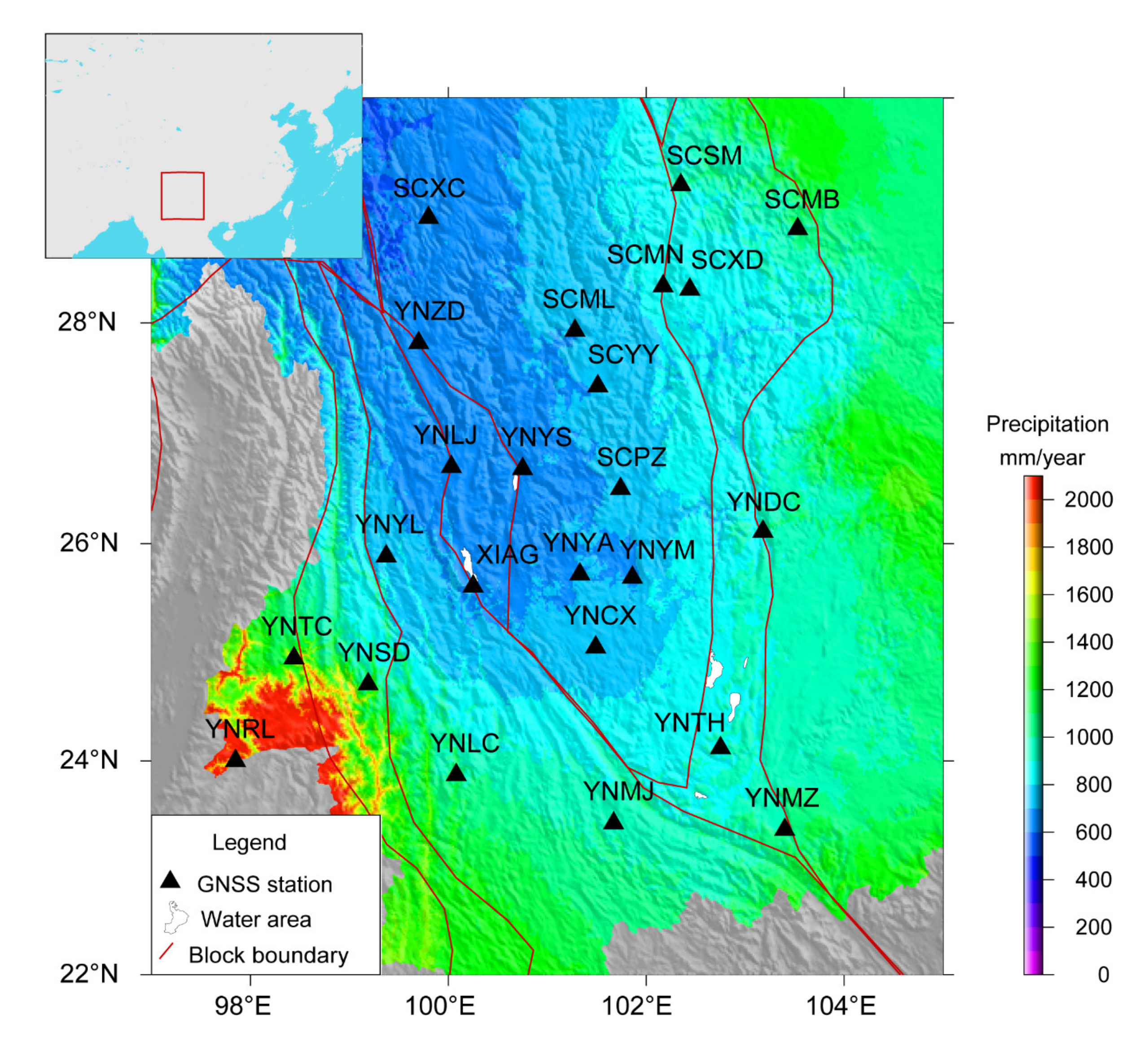
2.1.1. GNSS Data and Pre-Processing
2.1.2. GRACE Data and Processing
2.1.3. Precipitation Data
2.2. WT Method
3. Results
3.1. Periodic Term Composition Analysis
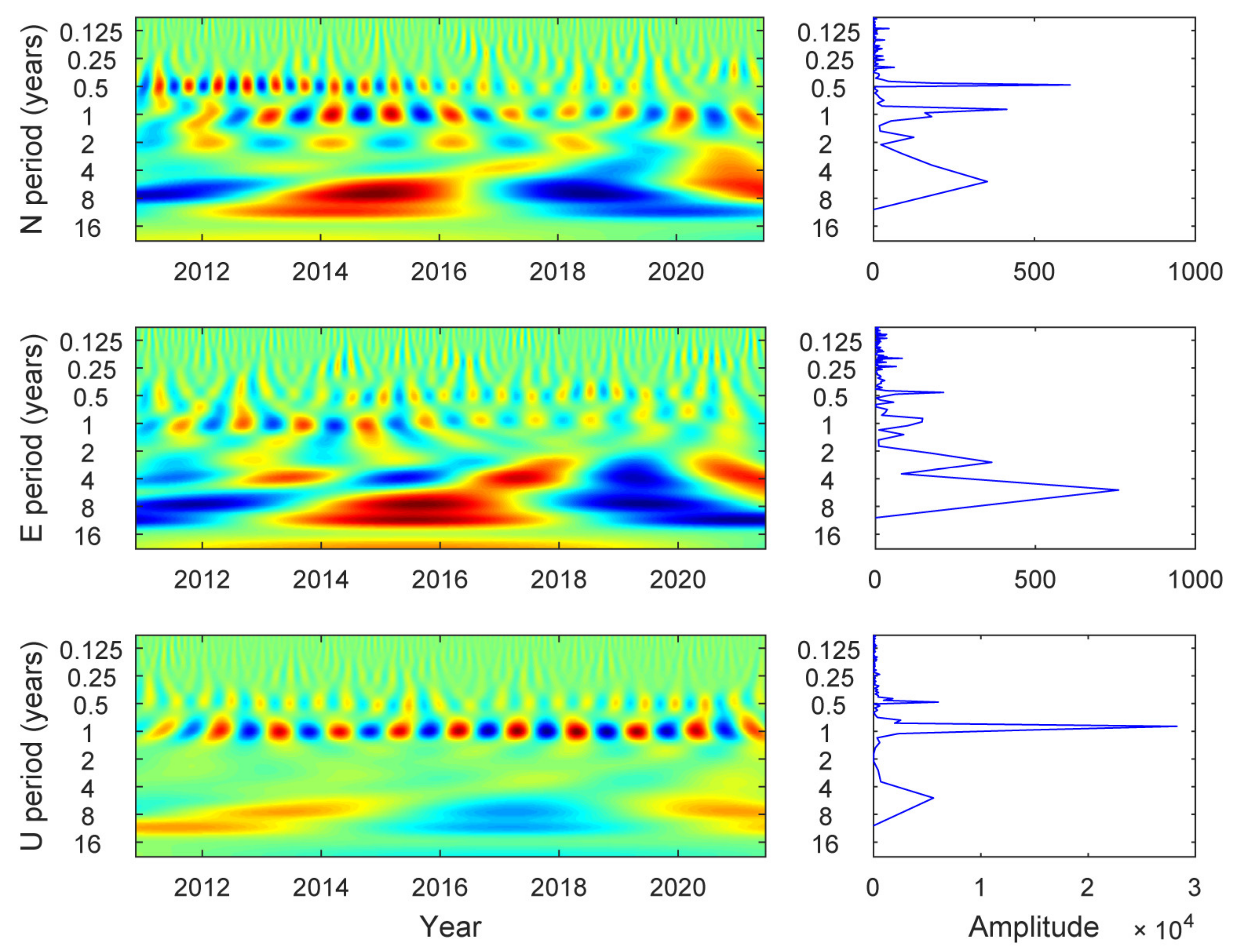
3.1.1. GNSS Data
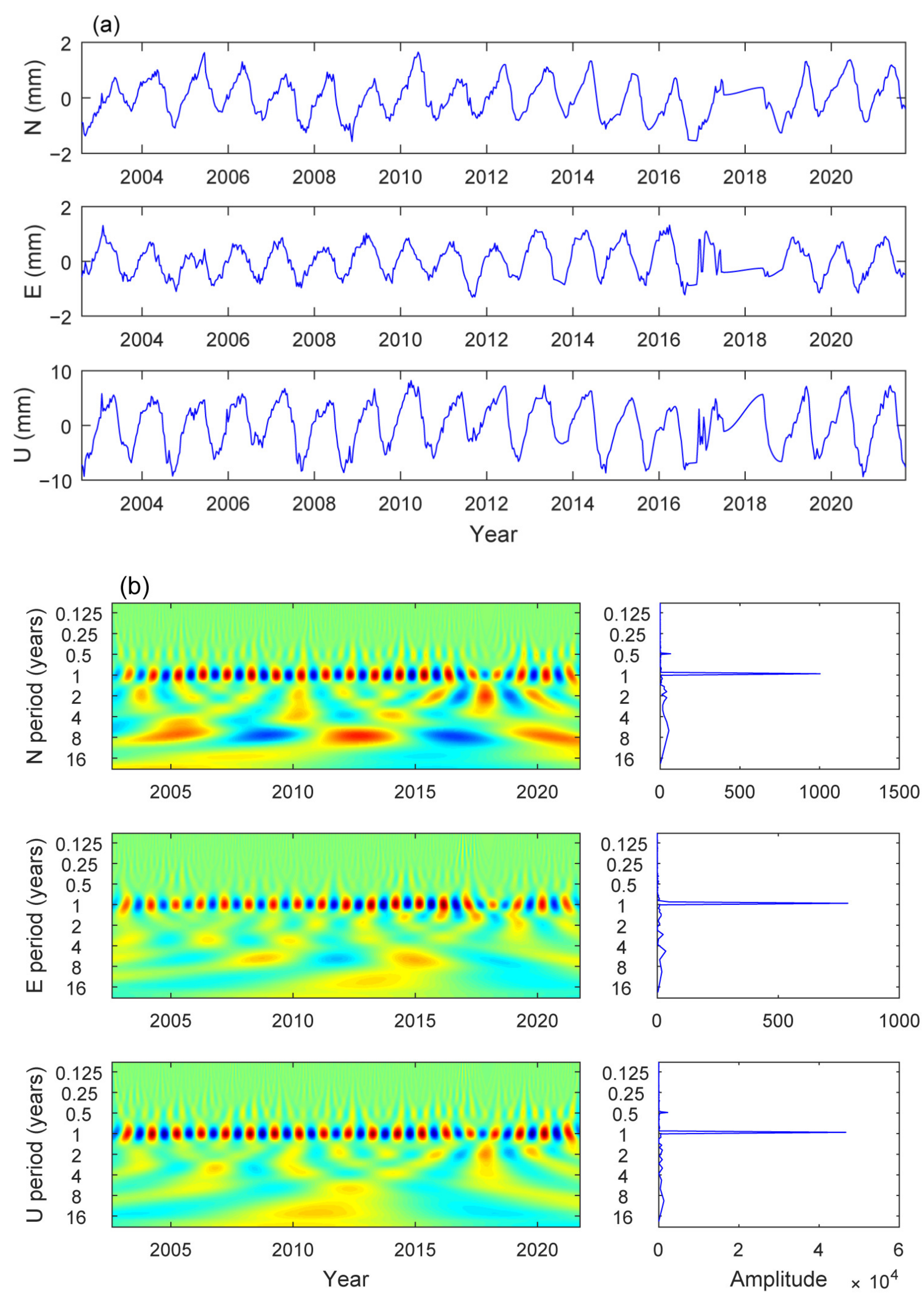
3.1.2. GRACE Data
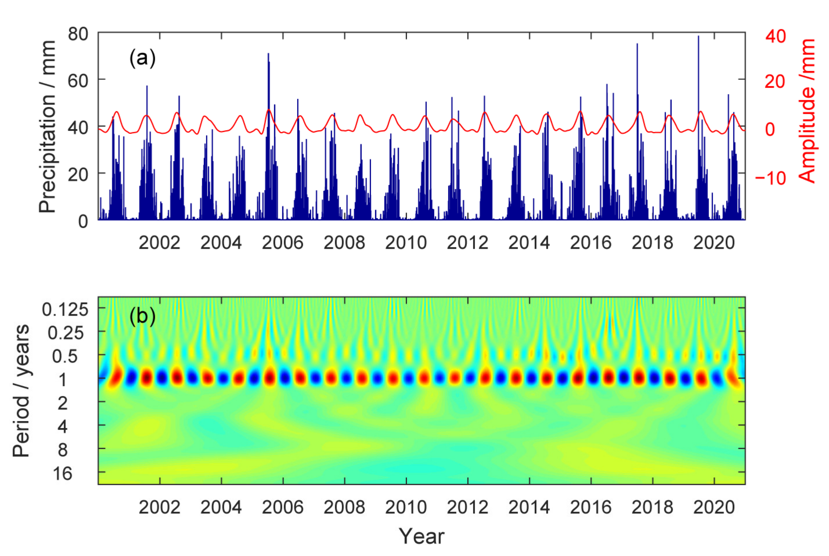
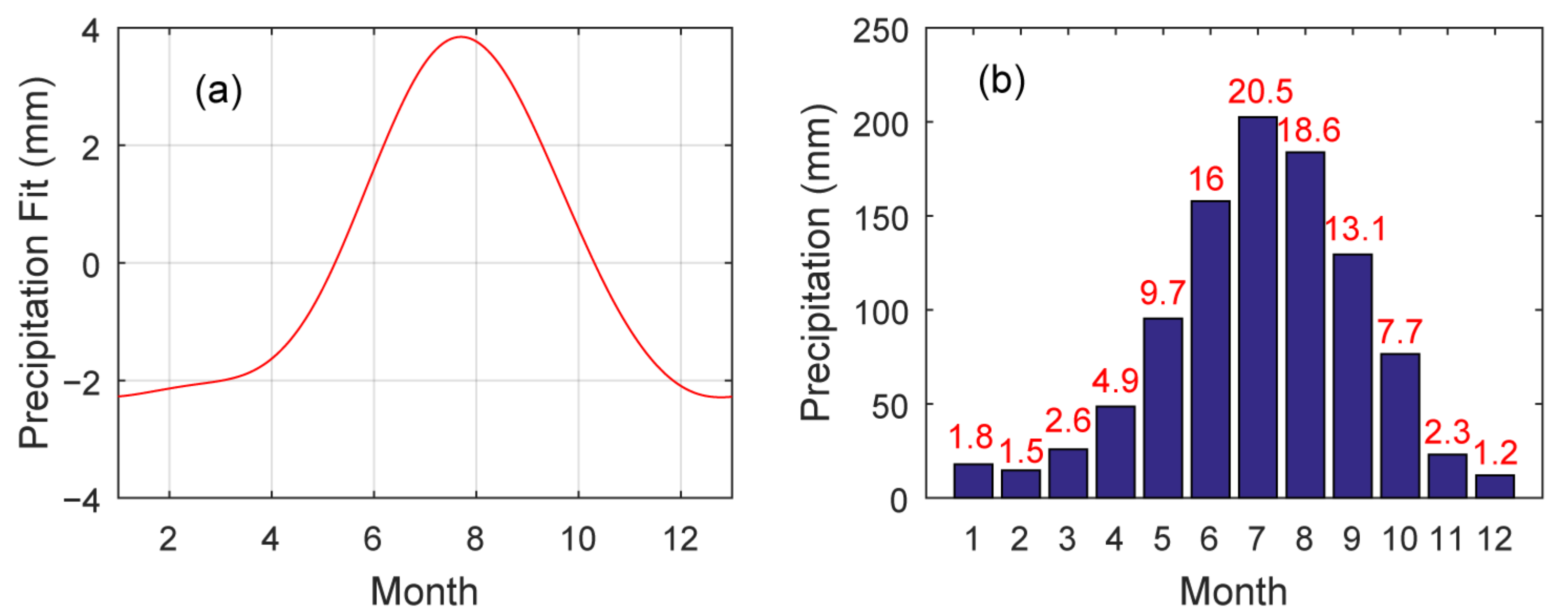
3.1.3. Precipitation Data
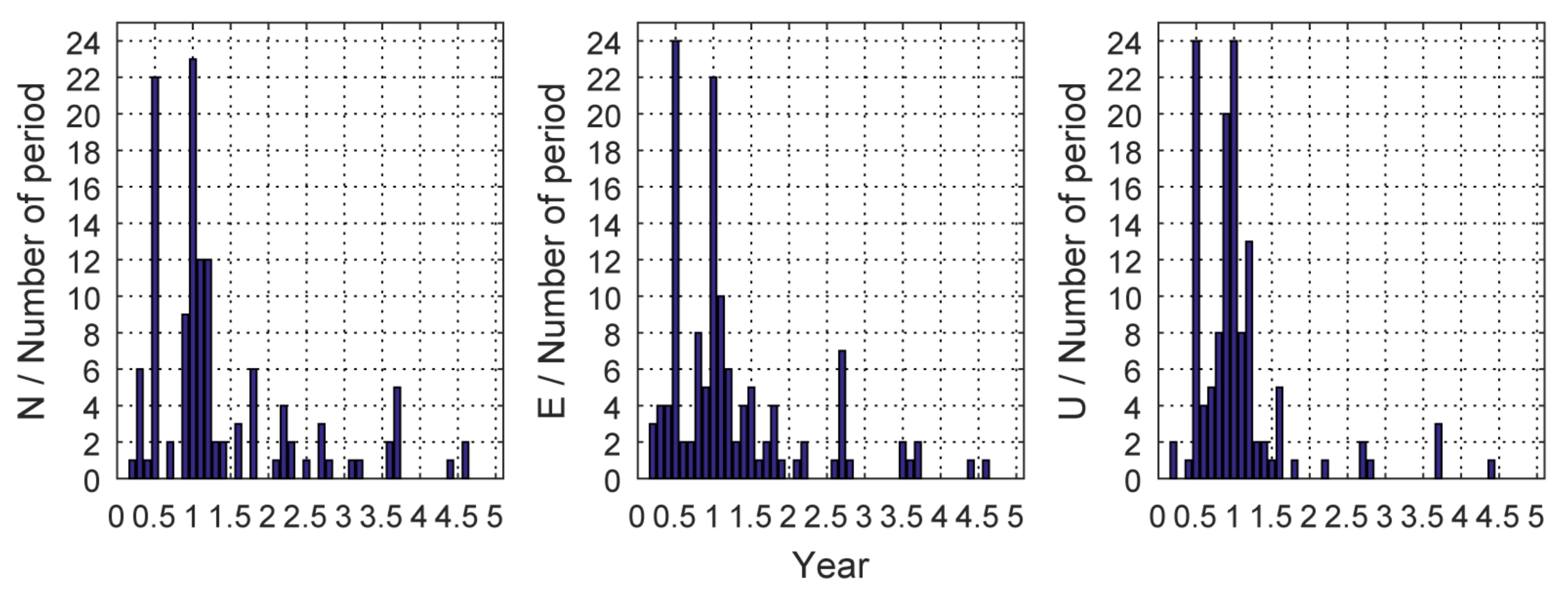
3.2. Seasonality Analysis
4. Discussion
5. Conclusions
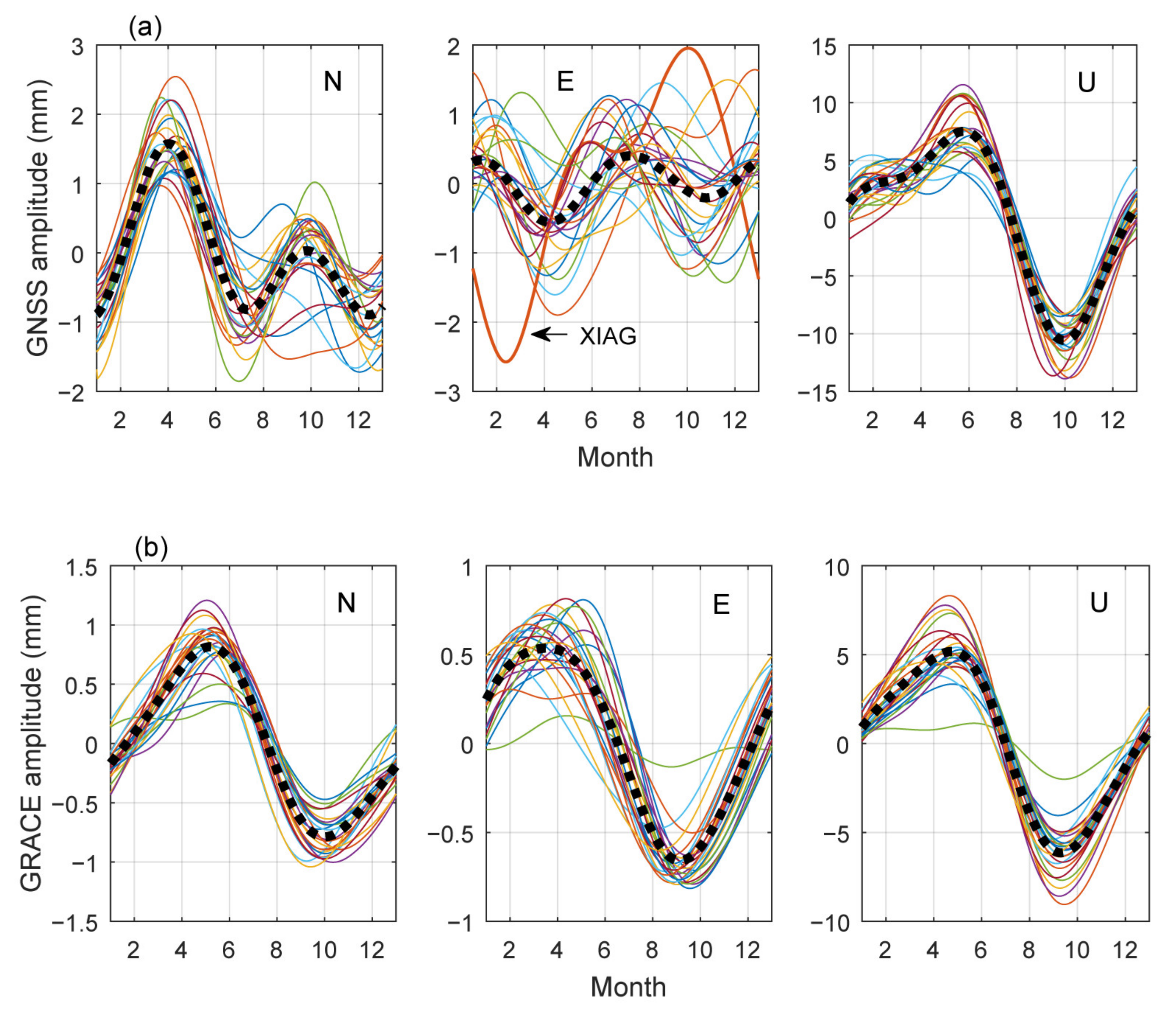
- The three data types for Sichuan and Yunnan have significant annual seasonality. The GNSS time series not only has a notable annual cycle but also an evident semi-annual cycle, and thus, the impact of the semi-annual cycle on the horizontal component should not be overlooked. Moreover, there are other shorter and longer periodic signals.
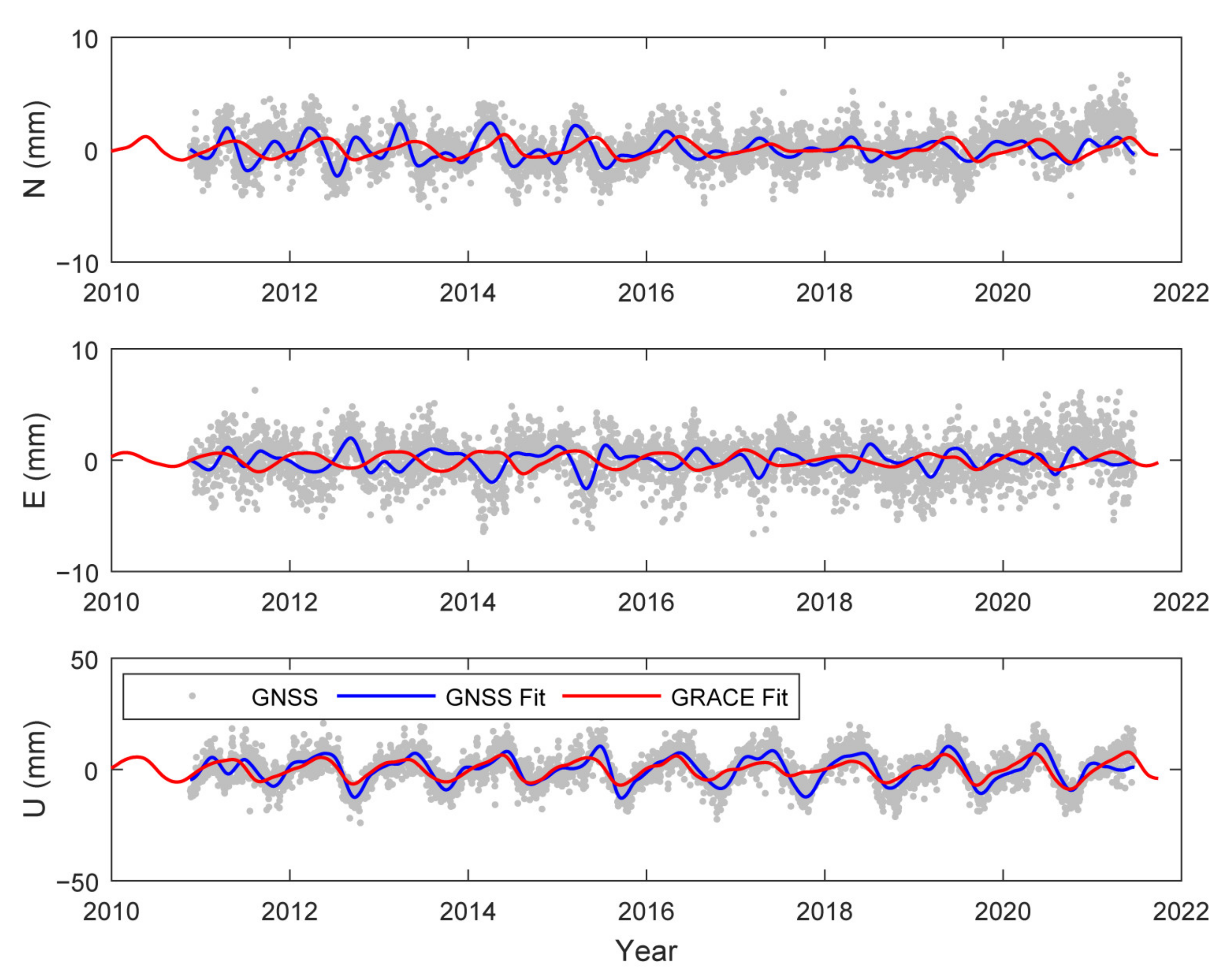
- A comparative analysis of GNSS and GRACE revealed that the vertical components are largely consistent, but the horizontal components differed considerably. GRACE provides comprehensive observation results for large areas, and has better vertical resolution than horizontal resolution. Regarding the actual observations, GNSS was affected by non-structural factors of large areas, and was easily influenced by the local observation environment.
- The seasonality of the vertical component of the GNSS three components was strong. The horizontal N component was stronger than the E component, and both were strongly negatively correlated. Seasonal deformation was mainly affected by instantaneous loading deformation and changes in the pore pressure due to precipitation.
- Regarding seasonal deformation, this study mainly discussed the influence of precipitation. Nevertheless, the GNSS observation stations were also affected by other factors, such as atmospheric pressure load, non-tidal ocean load, thermal expansion effect of bedrock at observation points, and data processing errors, which are also important factors that cause differences between GNSS and GRACE in terms of amplitude and phase.
- The correction of seasonal deformation of GNSS time series has important theoretical significance and application value for obtaining accurate information of surface movement and accurate use of observation data.
- Through the integrated application of GNSS and GRACE, it can also effectively monitor the regional land water storage changes or precipitation changes, and make up for the lack of weakness of professional technical means in some research areas.
Author Contributions
Funding
Institutional Review Board Statement
Informed Consent Statement
Data Availability Statement
Acknowledgments
Conflicts of Interest
References
- Farrell, W.E. Deformation of the Earth by Surface Loads. Rev. Geophys. Space Phys. 1972, 10, 761–797. [Google Scholar] [CrossRef]
- Wahr, J.; Khan, S.A.; van Dam, T.; Liu, L.; van Angelen, J.H.; Broeke, M.R.V.D.; Meertens, C.M. The use of GPS horizontals for loading studies, with applications to northern California and southeast Greenland. JGR Solid Earth 2013, 118, 1795–1806. [Google Scholar] [CrossRef] [Green Version]
- Jiang, W.P.; Li, Z.; Liu, H.F.; Zhao, Q. Cause Analysis of the Non-linear Variation of the IGS Reference Station Coordinate Time Series inside China. Chin. J. Geophys. 2013, 56, 2228–2237. [Google Scholar] [CrossRef]
- Chanard, K.; Avouac, J.P.; Ramillien, G.; Genrich, J. Modeling deformation induced by seasonal variations of continental water in the Himalaya region: Sensitivity to Earth elastic structure. JGR Solid Earth 2014, 119, 5097–5113. [Google Scholar] [CrossRef] [Green Version]
- Zhan, W.; Li, F.; Hao, W.F.; Yan, J.G. Regional characteristics and influencing factors of seasonal vertical crustal motions in Yunnan, China. Geophys. J. Int. 2017, 210, 1295–1304. [Google Scholar] [CrossRef]
- Ding, Y.H.; Huang, D.F.; Shi, Y.L.; Jiang, Z.S.; Chen, T. Determination of vertical surface displacements in Sichuan using GPS and GRACE measurements. Chin. J. Geophys. 2018, 61, 4777–4788. [Google Scholar] [CrossRef]
- Wang, M.; Sheng, Z.K. Present-day Tectonic Deformation in Continental China: Thirty Years of GPS Observation and Research. Earthq. Res. China 2020, 36, 660–683. [Google Scholar] [CrossRef]
- Liu, X.K.; Ding, Z.F.; Li, Y.; Liu, Z.G. Application of EMD in GNSS Time Series Periodic Term Processing. Geomat. Inf. Sci. Wuhan Univ. 2021. [Google Scholar] [CrossRef]
- Xiang, L.W.; Wang, H.S.; Steffen, H.; Wu, P.; Jia, L.L.; Jiang, L.M.; Shen, Q. Groundwater Storage Changes in the Tibetan Plateau and Adjacent Areas Revealed from GRACE Satellite Gravity Data. Earth Planet. Sci. Lett. 2016, 449, 228–239. [Google Scholar] [CrossRef] [Green Version]
- Wang, L.S.; Chen, C.; Zou, R.; Du, J.S.; Chen, X.D. Using GPS and GRACE to Detect Seasonal Horizontal Deformation Caused by Loading of Terrestrial Water: A Case Study in the Himalayas. Chin. J. Geophys. 2014, 57, 1792–1804. [Google Scholar] [CrossRef]
- Davis, J.L.; Elósegui, P.; Mitrovica, J.X.; Tamisiea, M.E. Climate-driven deformation of the solid Earth from GRACE and GPS. Geophys. Res. Lett. 2004, 31, L24605. [Google Scholar] [CrossRef] [Green Version]
- Fu, Y.N.; Donald, F.A.; Jeffrey, T.F.; Michael, B.H. Horizontal motion in elastic response to seasonal loading of rain water in the Amazon Basin and monsoon water in Southeast Asia observed by GPS and inferred from GRACE. Geophys. Res. Lett. 2013, 40, 6048–6053. [Google Scholar] [CrossRef]
- Chen, J.L.; Wilson, C.R.; Blankenship, D.; Tapley, B.D. Accelerated Antarctic Ice Loss from Satellite Gravity Measurements. Nat. Geosci. 2009, 2, 859–862. [Google Scholar] [CrossRef]
- Luthcke, S.B.; Arendt, A.A.; Rowlands, D.D.; McCarthy, J.J.; Larsen, C.F. Recent glacier mass changes in the Gulf of Alaska region from GRACE mascon solutions. J. Glaciol. 2008, 54, 767–777. [Google Scholar] [CrossRef] [Green Version]
- Ming, F.; Yang, Y.X.; Zeng, A.M.; Jing, Y.F. Analysis of Seasonal Signals and Long-Term Trends in the Height Time Series of IGS Sites in China. Sci. China Earth Sci. 2016, 46, 834–844. [Google Scholar] [CrossRef]
- Jiang, W.P.; Yuan, P.; Chen, H.; Cai, J.Q.; Li, Z. Annual Variations of Monsoon and Drought Detected by GPS: A Case Study in Yunnan, China. Sci. Rep. 2017, 7, 5874. [Google Scholar] [CrossRef]
- Zhan, W.; Li, J.W. Extraction and Analysis of the Common-Mode Component of GNSS Time Series in Yunnan. J. Seismol. Res. 2021, 44, 56–63. [Google Scholar]
- Liang, H.B.; Zhan, W.; Li, J.W. Vertical Surface Displacement of Mainland China from GPS Using the Multisurface Function Method. Adv. Space Res. 2021, 68, 4898–4915. [Google Scholar] [CrossRef]
- Herring, T.A.; King, R.W.; McClusky, S.C. GAMIT Reference Manual: GPS Analysis at MIT; Version 10.4; Massachusetts Institute of Technology: Cambridge, MA, USA, 2010. [Google Scholar]
- Van Dam, T.M.; Blewitt, G.; Heflin, M.B. Detection of atmospheric pressure loading using the Global Positioning System. JGR Solid Earth 1994, 99, 23939–23950. [Google Scholar] [CrossRef]
- Ponte, R.M.; Ray, R.D. Atmospheric pressure correction in geodesy and oceanography: A strategy for handling air tides. Geophys. Res. Lett. 2002, 29, 2153. [Google Scholar] [CrossRef]
- Dobslaw, H.; Thomas, M. Simulation and observation of global ocean mass anomalies. JGR Ocean. 2007, 112, C05040. [Google Scholar] [CrossRef]
- Shen, Y.Q.; Yan, H.M.; Peng, P.; Bai, X.F.; Tian, D.H. Comparative Study of Green’s Function and Spherical Harmonic Function Methods on Surface Deformation Caused by Mass Loading. Geomat. Inf. Sci. Wuhan Univ. 2017, 42, 1008–1014. [Google Scholar] [CrossRef]
- Guo, J.Y.; Li, Y.B.; Huang, Y.; Deng, H.T.; Xu, S.Q.; Ning, J.S. Green’s function of the deformation of the Earth as a result of atmospheric loading. Geophys. J. Int. 2004, 159, 53–68. [Google Scholar] [CrossRef] [Green Version]
- Bruinsma, S.; Lemoine, J.M.; Biancale, R.; Valès, N. CNES/GRGS 10-day gravity field models (release 02) and their evaluation. Adv. Space Res. 2010, 45, 587–601. [Google Scholar] [CrossRef]
- Torrence, C.; Compo, G.P. A practical guide to wavelet analysis. Bull. Am. Meteorol. Soc. 1998, 79, 61–78. [Google Scholar] [CrossRef] [Green Version]
- Xu, H.J.; Liu, L.T.; Hsu, H.T.; Sun, H.P. Wavelet approach to study the secular gravity variation. Chin. J. Geophys. 2008, 51, 735–742. [Google Scholar] [CrossRef]
- Li, J.W.; Song, X.D.; Yang, Y.; Li, M.K.; Li, J.T.; Li, Y.E. Strong seasonal variations of seismic velocity in eastern margin of Tibetan Plateau and Sichuan Basin from ambient noise interferometry. JGR Solid Earth 2021, 126, e2021JB022600. [Google Scholar] [CrossRef]
- Li, P. Analysis on adjustment of characteristic water level of Erhai Lake in Dali City. Pearl River 2008, 29, 46–48. [Google Scholar] [CrossRef]
- Liu, C.Y.; Aslam, K.S.; Daub, E.G. Seismic velocity changes caused by water table fluctuation in the New Madrid seismic zone and Mississippi embayment. JGR Solid Earth 2020, 125, e2020JB019524. [Google Scholar] [CrossRef]
- Jia, L.L.; Wang, Y.B.; Lian, W.P.; Xiang, L.W. Comparison and Analysis of Crustal Vertical Deformation in Mainland China Observed by GPS from CMONOC and GRACE. Acta Geod. Et Cartogr. Sin. 2018, 47, 899–906. [Google Scholar] [CrossRef]
- Liang, Y.; Qian, H.S.; Zhang, L. Regionalization of the annual precipitation change in the last 50 years in China (1961–2010). Acta Meteorol. Sin. 2016, 74, 31–45. [Google Scholar] [CrossRef]
- Xiong, M.Q. Climate regionalization and characteristics of daily precipitation in China in recent 60 years. Chin. J. Atmos. Sci. 2017, 41, 933–948. [Google Scholar] [CrossRef]
- Zhou, B.; Wang, C.X.; Zhang, S.Q. Quasi biennial Period Characteristics of Extreme Summer Drought Days and Its Possible Causes in Sichuan Basin During 1961–2018. J. Arid. Meteorol. 2021, 39, 727–733. [Google Scholar] [CrossRef]


| Station | N GNSS/GRACE | E GNSS/GRACE | U GNSS/GRACE | ||||||
|---|---|---|---|---|---|---|---|---|---|
| Phase (DOY) | Amplitude (mm) | CC | Phase (DOY) | Amplitude (mm) | CC | Phase (DOY) | Amplitude (mm) | CC | |
| SCMB | 112/130 | 1.84/0.90 | 0.63/0.94 | 24/131 | 1.76/0.65 | 0.28/0.94 | 169/115 | 7.01/3.63 | 0.85/0.95 |
| SCML | 81/127 | 1.44/1.02 | 0.35/0.96 | 360/46 | 2.10/0.57 | 0.67/0.94 | 142/113 | 11.55/4.95 | 0.93/0.96 |
| SCMN | 101/131 | 1.62/1.07 | 0.63/0.95 | 24/67 | 0.94/0.53 | 0.23/0.93 | 150/117 | 7.18/4.66 | 0.90/0.96 |
| SCPZ | 92/140 | 1.71/0.96 | 0.73/0.94 | 202/67 | 1.22/0.68 | 0.20/0.95 | 156/123 | 8.46/5.44 | 0.90/0.96 |
| SCSM | 103/150 | 1.71/0.42 | 0.63/0.91 | 226/117 | 1.41/0.23 | 0.57/0.52 | 153/145 | 7.85/1.66 | 0.89/0.84 |
| SCXC | 86/106 | 2.01/0.91 | 0.65/0.96 | 240/19 | 1.86/0.49 | 0.85/0.94 | 30/88 | 6.92/4.31 | 0.89/0.96 |
| SCXD | 102/132 | 2.01/1.07 | 0.66/0.95 | 216/93 | 1.20/0.56 | 0.28/0.93 | 136/119 | 7.69/4.63 | 0.84/0.96 |
| SCYY | 95/132 | 2.23/1.01 | 0.77/0.95 | 17/51 | 1.17/0.62 | 0.14/0.94 | 144/117 | 9.16/5.19 | 0.89/0.96 |
| XIAG | 99/125 | 1.91/1.08 | 0.53/0.95 | 275/75 | 2.79/0.76 | 0.60/0.96 | 146/111 | 9.50/6.42 | 0.84/0.97 |
| YNCX | 92/135 | 2.37/0.86 | 0.61/0.92 | 160/87 | 1.62/0.82 | 0.29/0.96 | 153/123 | 10.13/6.09 | 0.89/0.96 |
| YNDC | 87/149 | 1.71/0.87 | 0.58/0.91 | 197/127 | 1.83/0.74 | 0.46/0.95 | 128/130 | 7.89/5.15 | 0.86/0.95 |
| YNLC | 83/122 | 2.38/0.95 | 0.76/0.94 | 15/96 | 2.00/0.74 | 0.51/0.95 | 145/114 | 11.83/7.89 | 0.87/0.97 |
| YNLJ | 92/119 | 2.56/1.07 | 0.66/0.96 | 23/53 | 1.23/0.66 | 0.59/0.96 | 148/100 | 8.79/5.71 | 0.86/0.97 |
| YNMJ | 87/120 | 1.40/0.73 | 0.51/0.87 | 166/95 | 1.52/0.87 | 0.41/0.96 | 151/120 | 10.63/6.73 | 0.92/0.96 |
| YNMZ | 102/138 | 1.72/0.54 | 0.47/0.79 | 175/126 | 1.75/0.91 | 0.52/0.96 | 89/126 | 7.66/5.18 | 0.84/0.93 |
| YNRL | 77/135 | 2.11/1.08 | 0.63/0.96 | 173/143 | 1.88/0.43 | 0.45/0.86 | 140/113 | 11.16/8.93 | 0.92/0.98 |
| YNSD | 96/123 | 1.90/1.22 | 0.62/0.96 | 26/94 | 1.48/0.64 | 0.33/0.94 | 139/109 | 9.07/8.04 | 0.94/0.98 |
| YNTC | 89/124 | 1.76/1.35 | 0.57/0.97 | 253/109 | 1.63/0.52 | 0.01/0.92 | 145/108 | 13.01/8.29 | 0.91/0.98 |
| YNTH | 92/140 | 1.79/0.65 | 0.67/0.84 | 181/116 | 1.24/0.85 | 0.59/0.96 | 143/128 | 8.04/5.61 | 0.84/0.94 |
| YNYA | 84/136 | 1.85/0.92 | 0.75/0.94 | 29/77 | 1.25/0.77 | 0.35/0.96 | 150/122 | 8.73/5.82 | 0.87/0.96 |
| YNYL | 96/119 | 2.37/1.24 | 0.82/0.97 | 356/71 | 1.44/0.65 | 0.29/0.95 | 142/102 | 12.11/6.77 | 0.85/0.97 |
| YNYM | 94/142 | 1.68/0.88 | 0.40/0.93 | 210/85 | 1.67/0.74 | 0.49/0.95 | 157/126 | 9.37/5.68 | 0.80/0.96 |
| YNYS | 101/127 | 2.75/0.99 | 0.82/0.95 | 215/57 | 1.00/0.69 | 0.23/0.96 | 135/111 | 9.26/5.49 | 0.90/0.97 |
| YNZD | 89/107 | 2.22/1.01 | 0.62/0.97 | 326/30 | 2.15/0.58 | 0.44/0.95 | 150/85 | 7.99/5.04 | 0.78/0.96 |
| Mean Value | 93/130 | 1.96/0.95 | 0.63/0.93 | 170/85 | 1.59/0.66 | 0.41/0.93 | 139/115 | 9.21/5.72 | 0.87/0.96 |
Publisher’s Note: MDPI stays neutral with regard to jurisdictional claims in published maps and institutional affiliations. |
© 2022 by the authors. Licensee MDPI, Basel, Switzerland. This article is an open access article distributed under the terms and conditions of the Creative Commons Attribution (CC BY) license (https://creativecommons.org/licenses/by/4.0/).
Share and Cite
Liu, X.; Liang, H.; Ding, Z. Analyzing the Seasonal Deformation of the Sichuan–Yunnan Region Using GNSS, GRACE, and Precipitation Data. Appl. Sci. 2022, 12, 5675. https://doi.org/10.3390/app12115675
Liu X, Liang H, Ding Z. Analyzing the Seasonal Deformation of the Sichuan–Yunnan Region Using GNSS, GRACE, and Precipitation Data. Applied Sciences. 2022; 12(11):5675. https://doi.org/10.3390/app12115675
Chicago/Turabian StyleLiu, Xikang, Hongbao Liang, and Zhifeng Ding. 2022. "Analyzing the Seasonal Deformation of the Sichuan–Yunnan Region Using GNSS, GRACE, and Precipitation Data" Applied Sciences 12, no. 11: 5675. https://doi.org/10.3390/app12115675