Specific Emitter Identification Based on Ensemble Neural Network and Signal Graph

Abstract

Specific emitter identification (SEI) is a technology for extracting fingerprint features from a signal and identifying the emitter. In this paper, the author proposes an SEI method based on ensemble neural networks (ENN) and signal graphs, with the following innovations: First, a signal graph is used to show signal data in a non-Euclidean space. Namely, sequence signal data is constructed into a signal graph to transform the sequence signal from a Euclidian space to a non-Euclidean space. Hence, the graph feature (the feature of the non-Euclidean space) of the signal can be extracted from the signal graph. Second, the ensemble neural network is integrated with a graph feature extractor and a sequence feature extractor, making it available to extract both graph and sequence simultaneously. This ensemble neural network also fuses graph features with sequence features, obtaining an ensemble feature that has both features in Euclidean space and non-Euclidean space. Therefore, the ensemble feature contains more effective information for the identification of the emitter. The study results demonstrate that this SEI method has higher SEI accuracy and robustness than traditional machine learning methods and common deep learning methods.

1. Introduction

Specific emitter identification (SEI) is a process to extract individual features from signals of the same model and batch of communication emitters and identify the specific emitter [1]. The manufacturing process of emitters is random, so emitters, even of the same model and batch, do not have completely identical electrical characteristics [2]. With different electrical parameters, each emitter has unique characteristics and is thus called a fingerprint. The fingerprint characteristics [3] of the signal are due to the effects of in-phase and quadrature-phase imbalance(IQ imbalance), phase noise, harmonic distortion, and nonlinear distortion [4]. As the fingerprint of an emitter is unique, steady, and difficult to imitate, SEI based on the fingerprint feature extracted from an emitter is an effective method to identify the identity of the communication emitter.

The SEI methods can be divided into two categories: manual-feature-based methods and deep learning-based methods. Manual-feature-based methods extract manual features from the emitter signal and then use the machine learning classifier to Identify the specific emitter. Different from manual-feature-based methods, the deep learning-based methods automatically extract the features of the specific emitter signal to perform specific emitter identification.

At present, various methods have already been proposed for extracting the features of an emitter signal [5]. Specifically, the features obtained by spectral analysis of the signal include power spectrum features [6], frequency spectrum features [7], Hilbert spectrum features [8], and variational mode decomposition spectrum features [9]. The features generated in modulation–demodulation include non-linear features of the power amplifier [10], phase error, IQ offset [11], and carrier frequency offset [12,13]. Moreover, there are also many other emitter signal feature extraction and identification methods. For example, in [6], SEI was realized by extracting the signal’s fractal feature. In [14], the authors put forward an FID model for mathematical modeling of an emitter based on the emitter type and used this model to identify the undetermined signal. Wong et al. clustered IQ signals directly to identify specific emitters [15].

However, the manual feature extraction-based method has many shortcomings: First, the SEI system’s identification effect is limited by the effectiveness of the manual feature; additionally, the extraction of the manual feature necessitates that the researchers have sufficient prior knowledge of communication theory on emitters [4]. Second, this method has poor generalizability. A feature extraction method valid for the identification of one emitter is often invalid for the identification of other emitters. Hence, researchers usually need to find a new feature extraction method for identifying a new emitter. Third, many traditional SEI methods perform poorly and cannot meet the practical demands. Many recent studies have shown that deep learning outperformed traditional methods in SEI [16]. The shortcomings of traditional methods are being solved by deep learning.

Deep learning is undergoing rapid development and has been widely used in image processing, natural language processing, and speech recognition, obtaining excellent results. Currently, researchers are applying deep learning technology to SEI. Furthermore, some study results have proved that deep learning is feasible and has great potential in SEI. For example, T. O’Shea et al. [17] systematically analyzed the studies on deep neural networks in radio modulation identification. Robyns et al. [7] identified 22 LoRa devices in the multi-layer perceptron (MLP) and convolutional neural network (CNN) supervised learning methods. Sankhe et al. [18] identified five 802.11 protocol emitters by using CNN. Following that, Guanxiong Shen et al. identified 25 LoRa emitters by using CNN, MLP, and Long Short-Term Memory (LSTM), respectively. However, in the existing deep learning methods, signal features are generally extracted from Euclidean space directly, and then a simple neural network structure is used to identify the emitter. There is still a large room for improving the data representation and network structure.

To effectively extract the features of the signal, we propose signal graph (a new data representation method) and ensemble neural network (ENN). The main innovations in this paper are as follows:

(1)

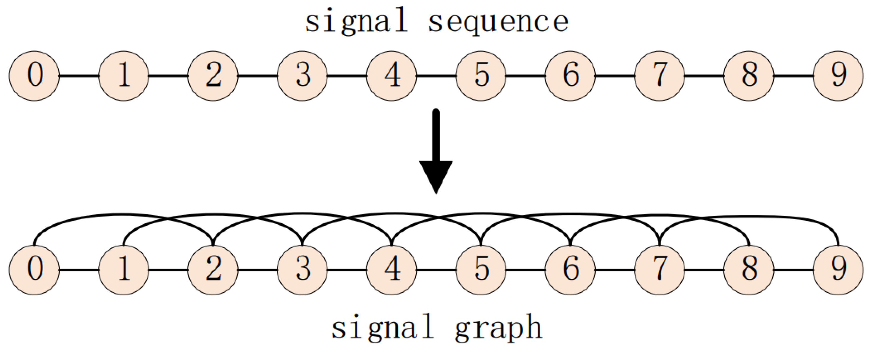
By constructing a signal graph, the sequence signal is transformed from a Euclidean space to a non-Euclidean space. As a result, the graph convolution method can be used to extract a signal’s non-Euclidean feature from its signal graph. Signal graph provides a new method, different from a signal sequence, for emitter signal representation.

(2)

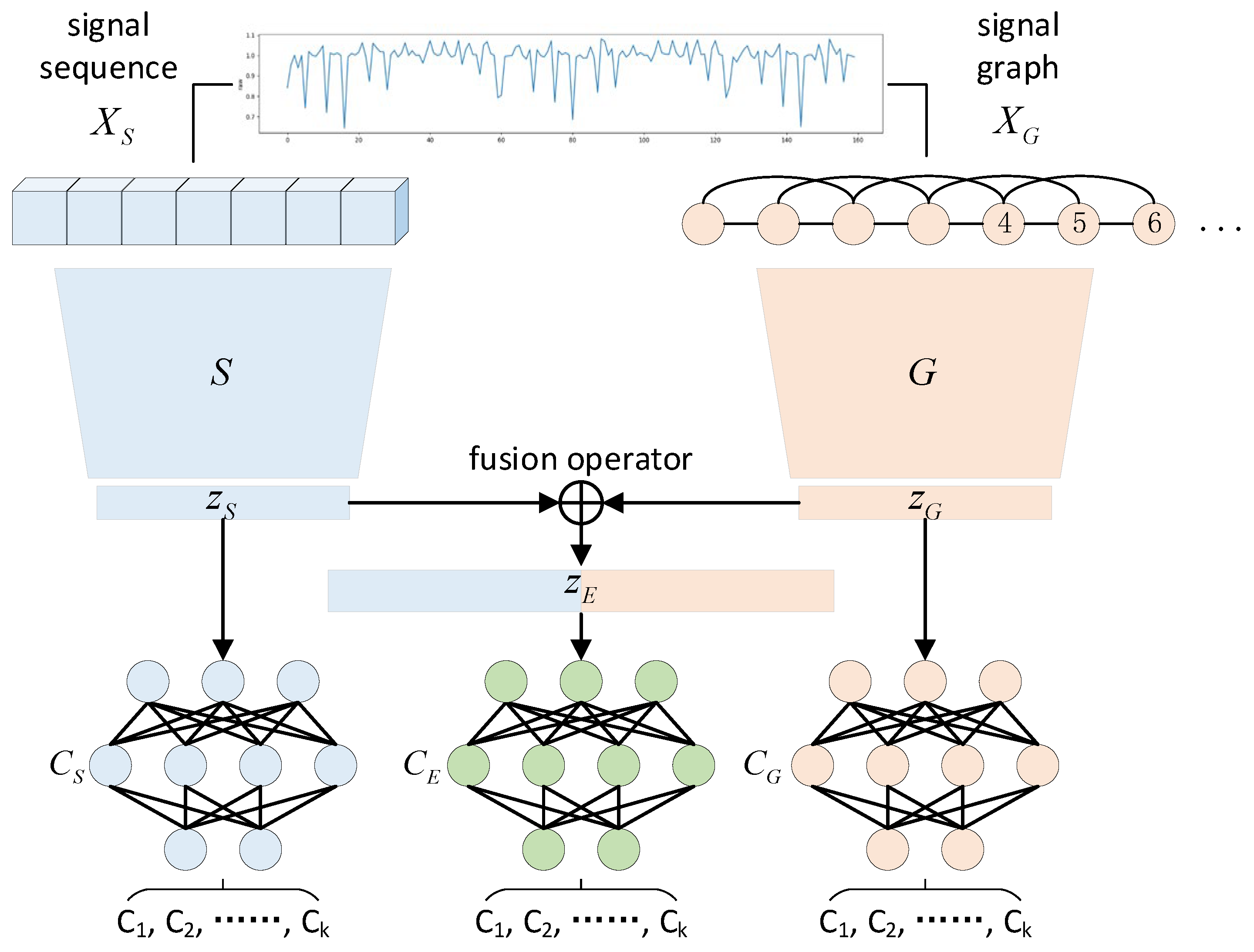
The ENN is designed with a sequence feature extractor and a graph feature extractor. Hence, it can extract sequence features from Euclidean space and graph features from non-Euclidean space and fuse the two features together to enrich the feature information extracted from the signal and better identify the emitter.

We conduct extensive experiments on ESP20 Dataset and RML2016a Dataset. Experimental results show that the proposed ENN outperforms the state-of-the-art methods for SEI tasks.

2. Ensemble Neural Network and Signal Graph-Based SEI

2.1. Signal Graph and Improved Graph Convolution

2.1.1. Signal Graph

An emitter signal can be input into a neural network directly or after being converted into another form. In this paper, the raw signal without any processing is called a signal sequence, which has two channels (i.e., components I and Q of the emitter signal) and a length of N. A signal sequence is data in Euclidean space; its elements are arranged as per the relations in the time sequence, and the geometric position relationships between the elements are specific. In order to represent the relationship between the nodes of a signal sequence, adjacent edges were added between the nodes to constitute a signal graph and obtain the signal sequence transformed from a Euclidean space to a non-Euclidean space. Then, a non-Euclidean feature of the signal can be extracted from the signal graph by graph convolution.

Figure 1 shows a signal sequence with a length of 10. The signal graph is constructed by adding adjacent edges between the nodes. After that, the nodes in the signal graph do not have the positional relationship in the signal sequence anymore but only the connection relationship.

2.1.2. Improved Graph Convolution for the Signal Graph

The formula for the original graph convolution can be defined as:

$$H^{l+1}=GConv(H,W)=\sigma \left(L{H}^l{W}^l\right)=\sigma \left(D^{-\frac{1}{2}}A{D}^{-\frac{1}{2}}{H}^l{W}^l\right)$$

(1)

where H is the output of the l-th layer graph convolution, W is the parameter matrix of the l-th layer graph convolution, A is the adjacency matrix of the graph, D is the degree matrix of the adjacency matrix A. In the original signal graph, all the adjacent nodes have the same impacts on the central node. However, different adjacent nodes have different impacts on the central node due to their different positions in the signal sequence [19].

In this regard, the standard graph convolution formula was improved in this study. Each adjacent edge of the adjacent matrix was given a weight parameter to adjust the impact of different adjacent nodes on the central node in the summation and updating. The weight parameter of the adjacent edge is determined by the following formula:

$$k\left(d\right)=\frac{1}{\sqrt{2\pi }}exp(-\frac{d^2}{2{\sigma }^2})$$

(2)

In the formula, k represents the weight parameter of the adjacent edge; d represents the distance between an adjacent node and the central node in the signal sequence; and $\sigma$ is the shape parameter. The distance between the adjacent node and the central node is inversely proportional to the impact of the former on the latter and vice versa. The set of the weight parameters is written as a weight matrix K ($length\times length$). The following formula exhibits the relation between the weight matrix K and the element $k_{ij}$:

$$K=\sum _{d\in [-160,160]}diag(length,d,k_{\left|d\right|})=\left[\begin{array}{cccccc}{k}_0& k_1& k_2& \cdots & k_{m-1}& k_m\\ k_1& k_0& k_1& \cdots & k_{m-2}& k_{m-1}\\ k_2& k_1& k_0& \cdots & k_{m-3}& k_{m-2}\\ ⋮& ⋮& ⋮& \ddots & ⋮& ⋮\\ k_{m-1}& k_{m-2}& k_{m-3}& \cdots & k_0& k_1\\ k_m& k_{m-1}& k_{m-2}& \cdots & k_1& k_0\end{array}\right]$$

(3)

In the formula, $diag$ is a diagonal matrix generator, where $length$ controls the dimensions of the diagonal matrix generated, d controls the position of the diagonal relative to the principal diagonal, $k_{\left|d\right|}$ controls the value of the diagonal element. Finally, weight matrix K and adjacent matrix A were used to calculate the Hadamard product and assign corresponding weight to each adjacent edge so as to control the impact of the different adjacent nodes on the central node in its updating. Therefore, the improved graph convolution for extracting features from the signal graph is written as the following formula:

$$H^{l+1}=Gonv(H,W)=\sigma (D^{-\frac{1}{2}}K\odot A{D}^{-\frac{1}{2}}{H}^l{W}^l)$$

(4)

where H is the output of the l-th layer graph convolution, W is the parameter matrix of the l-th layer graph convolution, A is the adjacency matrix of the graph, D is the degree matrix of the adjacency matrix A, and K is the proposed weight matrix.

2.2. The Proposed Ensemble Neural Network

In this study, an ensemble neural network (ENN) (Figure 2) was designed to make full use of sequence features and graph features, which are in two different spaces. It integrates sequence feature extractor with graph feature extractor and has a sequence classifier, a graph classifier, and an ensemble classifier.

Based on the two feature extractors, the ENN can extract sequence features in Euclidean space and graph features in non-Euclidean space from a signal sequence and a signal graph simultaneously and then fuse the two features together, obtaining the ensemble feature. As the ensemble feature contains the features in both Euclidean space and non-Euclidean space, it has more sufficient feature information for SEI than a single sequence feature or a graph feature.

The sequence classifier can identify a specific emitter based on the sequence feature extracted by the sequence feature extractor, and the graph classifier can identify a specific emitter based on the graph feature extracted by the graph feature extractor. However, the ensemble classifier can use the combination of sequence features and graph features to identify a specific emitter. The ENN treats the result obtained by the ensemble classifier as the final result. The sequence classifier and graph classifier support the training of ENN. Section 2.2.3 will show how to help the ENN obtain better SEI performance.

2.2.1. Components of the Modules

Sequence feature extractor: Sequence feature extractor is used to extract the features of the signal from Euclidean space. To this end, we use three cascaded convolutional layers with kernel size of 3 × 3 to form the feature extractor. In the selection the number of convolutional layers, we consider the overfitting and underfitting of the model. When the model capacity is too large, the model will over-fit, and when the model capacity is insufficient, the model is prone to under-fitting. In our model, three is a suitable value, which is obtained through cross-validation. In addition, the number of output channels of the three convolutional layers is set to 32, which is also the result of multiple attempts. Defining the sequence feature extractor as $S(·)$, the sequence signal as $X_s$, the output feature $z_S$ can be expressed as:

$$z_S=S\left(X_S\right)$$

(5)

Graph feature extractor: Graph feature extractor is used to extract the features of the signal from non-Euclidean space. Graph feature consists of one graph convolution layer (input layer) connected with two convolution layers with kernel size of 3 × 3. Corresponding to the sequence feature extractor, we also set the number of output channels of the graph convolutional layer and the convolutional layer to 32. Defining the graph feature extractor as $G(·)$, the sequence signal as $X_s$, the output feature $z_G$ can be expressed as:

$$z_G=G\left(X_S\right)$$

(6)

For the graph feature extractor, the first layer is the graph convolution layer, and the extracted feature is a graph, so the second layer cannot process graph structure data directly. In view of this state, the features extracted by the first layer can be transformed before being subjected to convolution. Specifically, all of the node connections in the graph feature are removed, and the node information is kept. Then, all of the nodes are reconstructed into a sequence based on their time sequences in the signal. Finally, the other two convolution layers are used to extract more of the feature and complete the extraction of the graph feature.

Feature fusion module: Feature fusion module is used to fuse $z_S$ and $z_G$, which can be written as:

$$z_E=\left[z_S,z_G\right]$$

(7)

where $[.]$ denotes feature concat, $z_E$ denotes the fused feature.

Classifier: Classifier is used to predict the classification results. To train the model efficiently, we classify and supervise the sequence feature, graph feature and fused feature. The classification results of the three classifiers can be expressed as:

$$p_S=C_S\left(z_S\right)$$

(8)

$$p_G=C_G\left(z_G\right)$$

(9)

$$p_E=C_E\left([{\mathrm{z}}_S,{\mathrm{z}}_G]\right)$$

(10)

where $C_s(.)$ denotes the sequence feature classifier, $C_G(.)$ denotes the graph feature classifier and $C_E(.)$ denotes the fused feature classifier. $P_S$, $P_G$, $P_E$ denotes the corresponding classification results, respectively. The three classifiers all adopt three-layer MLP structures, the number of neurons in each layer are 256, 80, and 20, respectively.

2.2.2. Loss Function

The ENN has three outputs which are from the sequence classifier, graph classifier, and ensemble classifier, respectively. In this paper, three sub-loss functions $L_S$, $L_G$ and $L_E$ are set for supervising the sequence classifier, graph classifier, and ensemble classifier, respectively. They are all cross-entropy loss functions as expressed in Formulas (11), (12), and (13), respectively:

$$L_S=-\frac{1}{N}\sum _{i=1}^N\sum _{j=1}^k{y}_{C_i}log\left[p_{y_{C_i}}\left(j\right)\right]$$

(11)

$$L_G=-\frac{1}{N}\sum _{i=1}^N\sum _{j=1}^k{y}_{G_i}log\left[p_{y_{G_i}}\left(j\right)\right]$$

(12)

$$L_E=-\frac{1}{N}\sum _{i=1}^N\sum _{j=1}^k{y}_{E_i}log\left[p_{y_{E_i}}\left(j\right)\right]$$

(13)

where N is the number of samples; k is the number of classes; y is the sample label; p is the result predicted by the model.

2.2.3. Training

The ENN was trained in two steps: local classifier supervision and global classifier supervision. In the first step, the outputs from the sequence classifier and the graph classifier were supervised by the loss functions at the same time. Hence, the total loss function $L_{step1}$ in this step was the sum of $L_S$ and $L_G$. The purpose was to enable the sequence/graph feature extractor and classifier to extract and classify corresponding features.

$$L_{step1}=L_S+L_G$$

(14)

The second step started after the training passed 90% of the whole epoch. In this step, the total loss function $L_{step2}$ include $L_S$, $L_G$, and $L_E$. Over the training in the first step, the sequence feature extractor and graph feature extractor of the ENN had been able to extract feature; on this basis, a good ensemble classifier was obtained just over a fine adjustment.

$$L_{step2}=L_S+L_G+L_E$$

(15)

To summarize, the ENN first used a sequence feature extractor and a graph feature extractor to extract sequence and graph features, respectively, and then fused the two features into an ensemble feature. During training, the first step was to supervise the outputs from the sequence classifier and the graph classifier to make the sequence feature extractor and the graph feature extractor able to extract corresponding features effectively. In the second step, the output from the ensemble classifier was also supervised, and the network was fine-tuned on the basis of the first step, obtaining the optimum SEI performance.

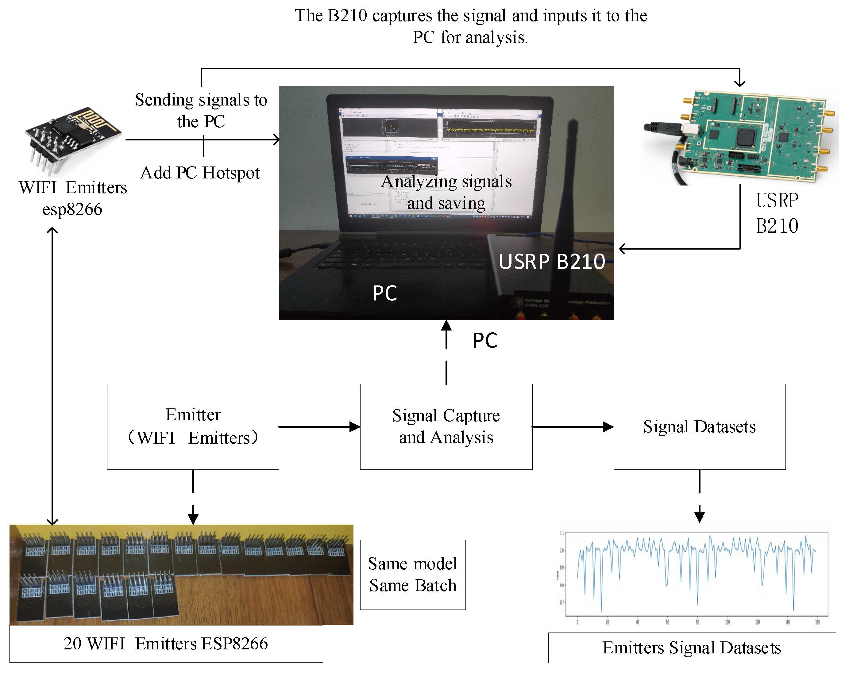
3. Experimental Data

ESP20 Dataset. ESP20 is a WIFI emitter signal dataset acquired by the authors. It contains the signal data acquired from 20 WIFI emitters of the same model (ESP8266) and batch. The acquisition process is presented in Figure 3. The dimension of each sample signal is 160 × 2. Specifically, 160 corresponds to the time dimension of the signal, and 2 corresponds to the in-phase and quadrature-phase of the signal.

RML2016a Dataset. An open-source RML2016a dataset was used to test the performance of ENN in emitter modulation method recognition. This dataset is a modulation signal dataset developed by O’Shea et al. using the GNU Radio signal simulation software [20]. Through this software, they generated 11 emitter signals with different modulation methods. The information of the ESP20 dataset and RML2016a dataset are summarized in

Table 1. Information summary of ESP20 dataset and RML2016a dataset.

Dataset Name	ESP20	RML2016a
Emitter model	WIFI device signal	Software simulation signal of different modulation method
Number of classes	20	11
Number of each class of samples	1300	1000
Sample size	Length = 160; number of channels = 2	Length = 128; number of channels = 2
Training set division	1–1000 per class is divided into training set	1–700 per class is divided into training set
Test set division	1001–1300 per class is divided into test set	701–1000 per class is divided into test set
Remarks	The 20 WIFI devices have the same model (ESP8266) and batch. The retained signal is the LLTF signal part in the complete WIFI signal.	The 11 modulation methods are 8PSK, AM-DSB, AM-SSB, BPSK, CPFSK, GFSK, PAM4, QAM16, QAM64, QPSK, and WBFM.

.

4. Experiment and Result Analysis

An SEI experiment was conducted on the self-acquired ESP20 dataset, and an emitter modulation method recognition experiment was carried out on the open source RML2016a dataset. The evaluation indicators of the experiment include accuracy, precision, recall, F1-score, and confusion matrix. The first experiment followed the following steps: First, noiseless raw data was used to train the ENN; second, the above evaluation indicators were used to evaluate the basic performance of the network; third, the additive white Gaussian noise was used to adjust the SNR of the data and test the robustness of the network at different SNRs. In the second experiment, as there was no noiseless raw signal, the different noise modulation signals provided in the dataset were directly used to train the ENN, which then was tested by the test set signal corresponding to the SNR.

Comparison methods. To demonstrate the superiority of the method proposed in this paper, the ENN was compared with two deep learning methods and two traditional machine learning methods in the experiment. For the deep learning method, we compare our model with CNN and GCN. The structure of CNN is consistent with the network structure constituted by the sequence feature extractor and sequence classifier of the ENN, while the structure of GCN accords with the network structure constituted by the graph feature extractor and graph classifier of the ENN. Therefore, GCN and CNN are not only state-of-the-art deep-learning based classifiers, but also part of our model. The comparison with CNN and GCN is also an ablation study of the effectiveness of the ENN structure. In addition, the ENN was also compared with the traditional decision tree and k-Nearest Neighbor algorithms. Both KNN and tree are implemented using sklearn. For the KNN algorithm, we select all samples in the training set as known classes, select all samples in the test set as test samples, and set the value of K to 3. For the decision tree method, we adopted the default values from sklearn. For CNN and GCN, the number of network layers and the number of neurons use the configuration described in Section 2.2.1. All hyperparameters are obtained by cross-validation. The results showed that the method proposed in this paper has better SEI performance than traditional methods and existing deep learning methods.

Training details. The ENN was trained in two steps. During training, the ENN was tested and trained on an NVIDIA GeForce GTX 950M GPU based on the PyTorch deep learning framework under Windows 10. The entire network was optimized by an ADAM optimizer with an initial learning rate of 0.001 and 50 epochs of iteration. It should be noted that in the experiments on the ESP20 dataset, the ENN was trained with a noiseless raw signal merely and tested with signals of various SNRs.

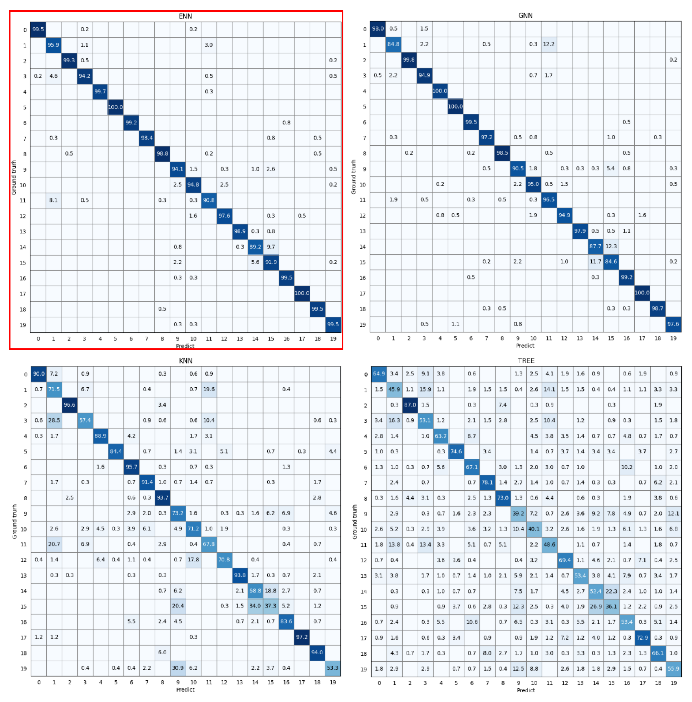
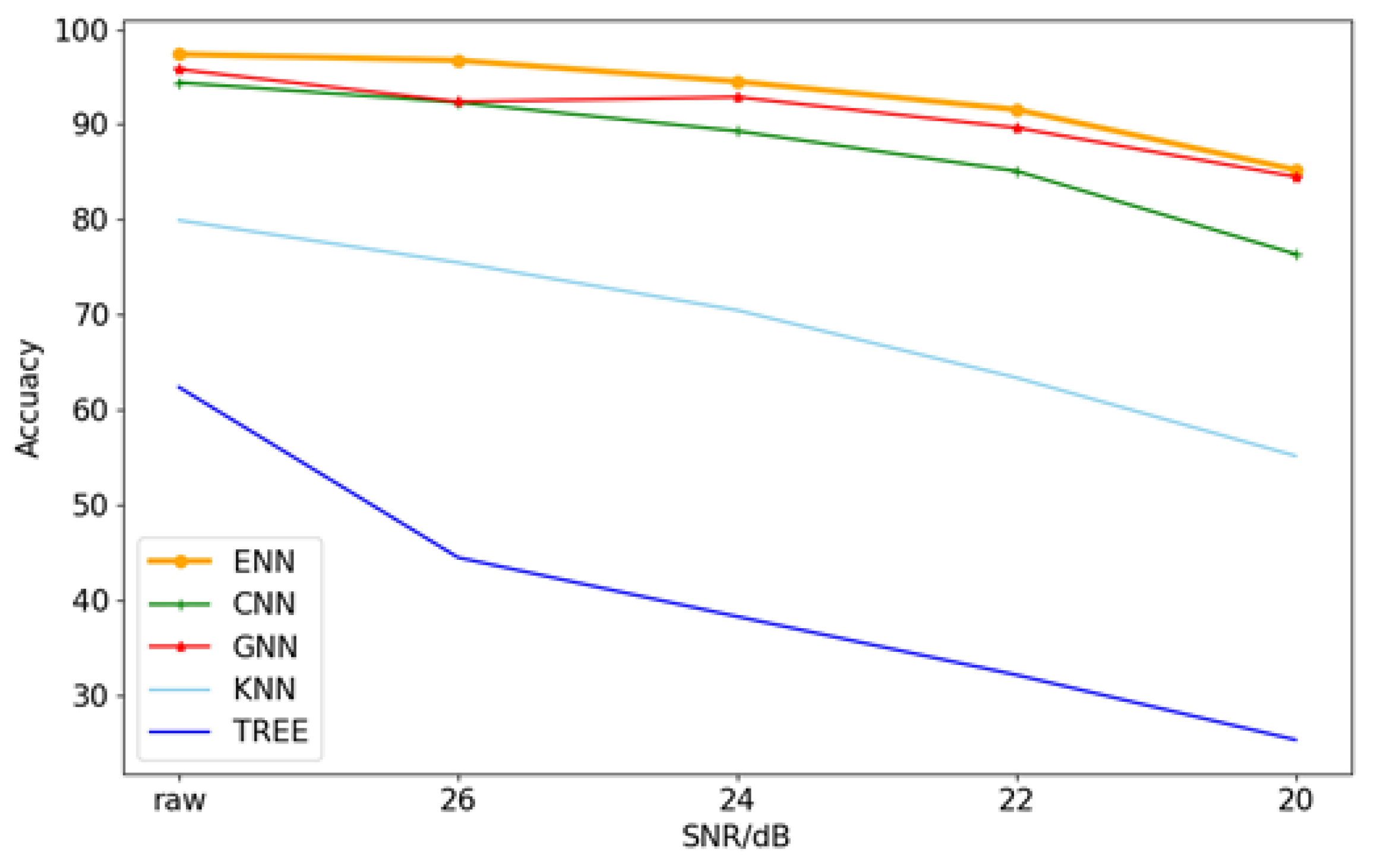
4.1. Results of SEI Experiment on the ESP20 Dataset

(1) Analysis of comprehensive performance indicators. This section analyzes the evaluated comprehensive indicators and robustness of the proposed method for the ESP20 dataset.

Table 2. A Summary of the evaluated indicators of different methods at various SNRs. Experimental results of our model are bolded.

SNR	Index	ENN	CNN	GCN	KNN	TREE
raw	Accuracy	97.38	94.4	95.78	79.91	62.9
	Precision	97.33	93.76	94	80.61	63.17
	Recall	97.41	93.56	94.45	79.79	62.77
	F1-Score	97.14	93.08	93.47	79.68	62.71
26 dB	Accuracy	96.73	92.31	92.38	84.52	47.23
	Precision	96.07	93.76	94.33	85.14	47.65
	Recall	98.53	95.61	92.41	84.73	47.19
	F1-Score	96.7	93.98	91.84	84.48	47.37
24 dB	Accuracy	94.51	89.3	92.87	85.18	41.67
	Precision	96.2	89.96	94.85	86.06	41.6
	Recall	95.69	88.56	95.7	85.02	41.57
	F1-Score	95.22	88.13	93.93	85.09	41.53
22 dB	Accuracy	91.56	85.1	89.65	84.12	34.47
	Precision	93.55	81.03	84.29	84.72	34.31
	Recall	93.37	83.94	80.68	83.95	34.53
	F1-Score	92.21	80.44	80.68	83.86	34.36
20 dB	Accuracy	85.23	76.38	84.51	83.23	25.55
	Precision	90.62	74.44	84.64	84.07	25.42
	Recall	89.27	71	82.06	83.2	25.56
	F1-Score	88.97	70.02	80.03	83.16	25.33

lists the experimental results of different evaluation indicators of the proposed method and other comparison methods at various SNRs. The optimum results have been bolded. As shown in Table 2, ENN had optimum performance in four evaluation indicators compared with other comparison methods. GCN performed second in the indicators, which was better than CNN. Through a comparison between GCN and CNN, it is concluded that the signal graph proposed in this paper is effective for signal data representation. Moreover, ENN performed better than CNN and GCN in SEI, which indicated that ENN can effectively extract the fingerprint feature of a signal and identify the specific emitter. Figure 4 shows the confusion matrices of the methods, where the pixels of ENN concentrate on the diagonal clearly, while those of the confusion matrix of the comparison methods are distributed beyond the diagonal area vaguely. This case intuitively explains that the ENN has the optimum SEI performance.

(2) Robustness analysis at various SNRs. As shown in Table 2, the classification indicators of the ENN were obviously superior to those of CNN and GCN at different SNRs. Figure 5 illustrates that the proposed method has higher accuracy than the comparison methods at all the SNRs. This proves that this method has excellent robustness at different SNRs. Especially in poor signal environments, for example, when the SNR was 20 dB, the experimental results better reflected the robustness of the proposed method. At this time, the identification accuracy of CNN was 76.38%, that of GCN was 84.51%, and that of the proposed method was 85.23%. The accuracy of GCN based on signal graph and improved graph convolution was about 8% higher than that of CNN, which implied that signal graph was effective for representing signal data. Meanwhile, the accuracy of ENN was about 1% higher than that of GCN, further indicating the excellent robustness of ENN.

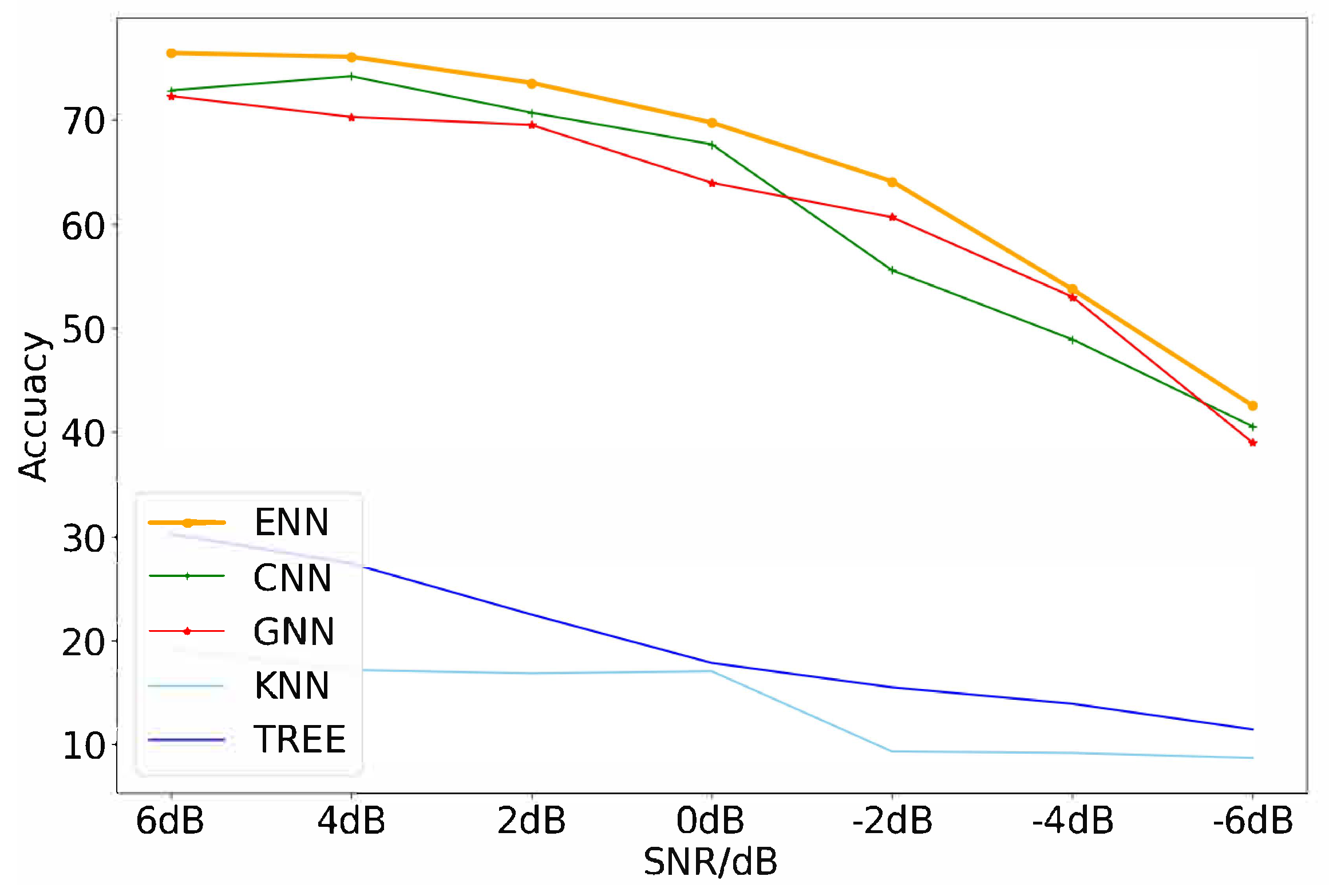
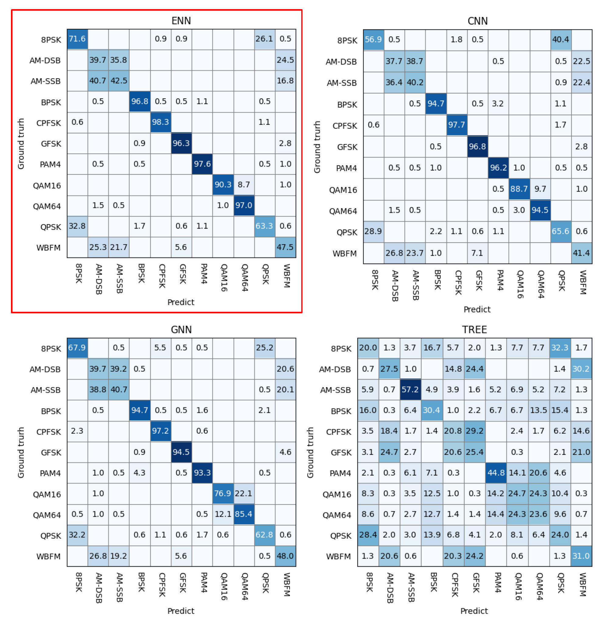
4.2. Results of Emitter Modulation Method Recognition Experiment on the RML2016a Dataset

This section analyzes the effectiveness of the proposed method for emitter modulation method identification based on the open source RML2016a dataset.

Table 3. Experimental results of the indicators at various SNRs. Experimental results of our model are bolded.

SNR	Index	ENN	CNN	GCN	KNN	TREE
6 dB	Accuracy	76.41	72.82	72.27	19.15	30.21
	Precision	77.61	72.55	72.09	25.09	30.84
	Recall	77.14	72.37	71.86	19.3	29.95
	F1-Score	77.24	72.41	71.87	16.28	30.31
4 dB	Accuracy	76.05	74.18	70.27	17.15	27.39
	Precision	76.63	73.81	69.98	26	27.96
	Recall	75.95	73.67	69.92	17.64	27.31
	F1-Score	76.07	73.71	69.86	15.06	27.54
2 dB	Accuracy	73.55	70.68	69.5	16.82	22.48
	Precision	73.63	71.48	70.28	25.76	22.96
	Recall	73.49	71.32	70.04	16.98	22.46
	F1-Score	73.49	71.29	70.1	14.46	22.59
0 dB	Accuracy	69.73	67.64	63.95	17.03	17.82
	Precision	70.43	67.77	63.98	23.51	18.26
	Recall	70.54	67.93	64.3	17.51	17.94
	F1-Score	70.38	67.79	64.07	12.29	18
−2 dB	Accuracy	64.09	55.55	60.64	9.33	15.48
	Precision	64.93	56	60.41	15.42	15.65
	Recall	64.68	55.57	60.59	9.17	15.55
	F1-Score	64.67	55.69	60.47	3.23	15.57
−4 dB	Accuracy	53.73	48.91	53	9.18	13.91
	Precision	53.07	48.78	53.1	10.09	14
	Recall	52.66	48.81	53.01	9.09	13.85
	F1-Score	52.84	48.77	53.04	1.82	13.88
−6 dB	Accuracy	42.55	40.55	39	8.7	11.45
	Precision	42.91	40.67	38.37	8.09	11.47
	Recall	42.94	40.27	38.68	9.09	11.56
	F1-Score	42.84	40.33	38.47	1.48	11.5

displays the emitter modulation method identification results of ENN and the comparison methods at various SNRs. The optimum results have been bolded. Figure 6 shows the accuracies of the methods at various SNRs. As the signals of the RML2016a dataset had low SNR as a whole, traditional methods became almost unable to identify the emitter based on the dataset, while the three deep learning methods (ENN, CNN, and GCN) still showed high robustness, with significantly higher accuracy than traditional machine learning methods. Figure 7 presents the confusion matrices of the methods, where the pixels of ENN are concentrated on the diagonal the most. This indicated that the proposed SEI method had optimum performance. The specific results are presented in Table 3.

As shown, the proposed method obtained the best accuracy, precision, recall, and F1-score. Both CNN and GCN have advantages. CNN performed better than GCN at high SNR, but was less robust than GCN at low SNR. In summary, the signal graph and ENN combined method proposed in this paper has excellent identification ability and robustness at various SNRs.

5. Conclusions

In view that the signals used in some existing studies were sourced from simulation software and the dataset was less representative in practice, the authors designed a WIFI emitter communication platform, acquired WIFI signals practically, and formulated the dataset. To fully extract fingerprint features from a signal, a signal graph was designed and used to have the signal sequence transformed from a Euclidean space to a non-Euclidean space; furthermore, an ensemble neural network (ENN) was designed, making it available to extract features from the signal sequence and signal graph simultaneously. Subsequently, the extracted sequence and graph features were fused together, forming an ensemble feature with richer information than a single sequence or graph feature. Finally, the ENN was trained in two steps. In the experiments, there were four comparison methods, including two traditional SEI methods (decision tree and k-nearest neighbor algorithms) and two deep learning SEI methods (CNN and GCN). Among them, CNN has the same network structure as the network structure formed by the sequence feature extractor and sequence classifier of the ENN, while GCN has a completely identical network structure to the network structure formed by the graph feature extractor and graph classifier of the ENN. Therefore, the experiment on CNN and GCN is an ablation study of the network modules of ENN, which can indicate the effectiveness of the modules. In the experiments, SEI was conducted on the ESP20 dataset, and emitter modulation method recognition was carried out on the open-source RML2016a dataset. The experimental results demonstrated that the proposed method performed the best in accuracy, precision, recall, and F1-score at various SNRs. This indicates that this method can effectively improve the SEI’s performance on the basis of CNN and GCN. Furthermore, the best performance of the proposed method at various SNRs proves that this method has the highest robustness, and the optimum performance of the method in different SEIs reveals that our method has high generalization.

References

1. Talbot, K.I.; Duley, P.R.; Hyatt, M.H. Specific emitter identification and verification. Technol. Rev. 2003, 113, 133. [Google Scholar]
2. Chen, Y.; Chen, X.; Lei, Y. Emitter Identification of Digital Modulation Transmitter Based on Nonlinearity and Modulation Distortion of Power Amplifier. Sensors 2021, 21, 4362. [Google Scholar] [CrossRef] [PubMed]
3. Kang, J.; Shin, Y.; Lee, H.; Park, J.; Lee, H. Radio Frequency Fingerprinting for Frequency Hopping Emitter Identification. Appl. Sci. 2021, 11, 10812. [Google Scholar] [CrossRef]
4. Sankhe, K.; Belgiovine, M.; Zhou, F.; Riyaz, S.; Ioannidis, S.; Chowdhury, K. ORACLE: Optimized radio classification through convolutional neural networks. In Proceedings of the IEEE INFOCOM 2019-IEEE Conference on Computer Communications, Paris, France, 29 April–2 May 2019; pp. 370–378. [Google Scholar]
5. Jiang, W.; Cao, Y.; Yang, L.; He, Z. A time-space domain information fusion method for specific emitter identification based on Dempster–Shafer evidence theory. Sensors 2017, 17, 1972. [Google Scholar] [CrossRef] [PubMed] [Green Version]
6. Zhu, M.; Zhang, X.; Qi, Y.; Ji, H. Compressed sensing mask feature in time-frequency domain for civil flight radar emitter recognition. In Proceedings of the 2018 IEEE International Conference on Acoustics, Speech and Signal Processing (ICASSP), Calgary, AB, Canada, 15–20 April 2018; pp. 2146–2150. [Google Scholar]
7. Robyns, P.; Marin, E.; Lamotte, W.; Quax, P.; Singelée, D.; Preneel, B. Physical-layer fingerprinting of LoRa devices using supervised and zero-shot learning. In Proceedings of the 10th ACM Conference on Security and Privacy in Wireless and Mobile Networks, Boston, MA, USA, 18–20 July 2017; pp. 58–63. [Google Scholar]
8. Zhang, J.; Wang, F.; Dobre, O.A.; Zhong, Z. Specific emitter identification via Hilbert–Huang transform in single-hop and relaying scenarios. IEEE Trans. Inf. Forensics Secur. 2016, 11, 1192–1205. [Google Scholar] [CrossRef]
9. Satija, U.; Trivedi, N.; Biswal, G.; Ramkumar, B. Specific emitter identification based on variational mode decomposition and spectral features in single hop and relaying scenarios. IEEE Trans. Inf. Forensics Secur. 2018, 14, 581–591. [Google Scholar] [CrossRef]
10. Polak, A.C.; Dolatshahi, S.; Goeckel, D.L. Identifying wireless users via transmitter imperfections. IEEE J. Sel. Areas Commun. 2011, 29, 1469–1479. [Google Scholar] [CrossRef]
11. Brik, V.; Banerjee, S.; Gruteser, M.; Oh, S. Wireless device identification with radiometric signatures. In Proceedings of the 14th ACM International Conference on Mobile Computing and Networking, San Francisco, CA, USA, 14–19 September 2008; pp. 116–127. [Google Scholar]
12. Nguyen, N.T.; Zheng, G.; Han, Z.; Zheng, R. Device fingerprinting to enhance wireless security using nonparametric Bayesian method. In Proceedings of the 2011 Proceedings IEEE INFOCOM, Shanghai, China, 10–15 April 2011; pp. 1404–1412. [Google Scholar]
13. Liu, P.; Yang, P.; Song, W.Z.; Yan, Y.; Li, X.Y. Real-time identification of rogue WiFi connections using environment-independent physical features. In Proceedings of the IEEE INFOCOM 2019-IEEE Conference on Computer Communications, Paris, France, 29 April–2 May 2019; pp. 190–198. [Google Scholar]
14. Zheng, T.; Sun, Z.; Ren, K. FID: Function modeling-based data-independent and channel-robust physical-layer identification. In Proceedings of the IEEE INFOCOM 2019-IEEE Conference on Computer Communications, Paris, France, 29 April–2 May 2019; pp. 199–207. [Google Scholar]
15. Wong, L.J.; Headley, W.C.; Andrews, S.; Gerdes, R.M.; Michaels, A.J. Clustering learned CNN features from raw I/Q data for emitter identification. In Proceedings of the MILCOM 2018—2018 IEEE Military Communications Conference (MILCOM), Los Angeles, CA, USA, 29–31 October 2018; pp. 26–33. [Google Scholar]
16. Wu, L.; Zhao, Y.; Wang, Z.; Abdalla, F.Y.; Ren, G. Specific emitter identification using fractal features based on box-counting dimension and variance dimension. In Proceedings of the 2017 IEEE International Symposium on Signal Processing and Information Technology (ISSPIT), Bilbao, Spain, 18–20 December 2017; pp. 226–231. [Google Scholar]
17. West, N.E.; O’Shea, T. Deep architectures for modulation recognition. In Proceedings of the 2017 IEEE International Symposium on Dynamic Spectrum Access Networks (DySPAN), Baltimore, MD, USA, 6–9 March 2017; pp. 1–6. [Google Scholar]
18. Riyaz, S.; Sankhe, K.; Ioannidis, S.; Chowdhury, K. Deep learning convolutional neural networks for radio identification. IEEE Commun. Mag. 2018, 56, 146–152. [Google Scholar] [CrossRef]
19. Kipf, T.N.; Welling, M. Semi-supervised classification with graph convolutional networks. In Proceedings of the 5th International Conference on Learning Representations(ICLR), Toulon, France, 24–26 April 2017. [Google Scholar]
20. O’shea, T.J.; West, N. Radio machine learning dataset generation with gnu radio. In Proceedings of the GNU Radio Conference, Charlotte, NC, USA, 20–24 September 2016; Volume 1. [Google Scholar]
Figure 1. A signal graph constituted from a signal sequence.
Applsci 12 05496 g001
Figure 2. Structure of the ensemble neural network proposed in this paper.
Applsci 12 05496 g002
Figure 3. The production process of WIFI emitter communication platform and signal dataset.
Applsci 12 05496 g003
Figure 4. Confusion matrices of ENN and the comparison methods. The confusion matrix of our model has been highlighted with a red square. The stronger the blue color, the higher the classification accuracy.
Applsci 12 05496 g004
Figure 5. Accuracies of ENN and the comparison methods at various SNRs.
Applsci 12 05496 g005
Figure 6. Accuracies of the proposed method and the comparison methods at various SNRs.
Applsci 12 05496 g006
Figure 7. Confusion matrices of the proposed method and the comparison methods at SNR of 6 dB. The confusion matrix of our model has been highlighted with a red square. The stronger the blue color, the higher the classification accuracy.
Applsci 12 05496 g007