Surrogate Model-Based Parameter Tuning of Simulated Annealing Algorithm for the Shape Optimization of Automotive Rubber Bumpers

Featured Application

The developed surrogate model-based parameter tuning method of the simulated annealing algorithm is suitable for solving not only numerical simulation optimization problems but also other computationally intensive model-driven optimizations.

Abstract

A design engineer has to deal with increasingly complex design tasks on a daily basis, for which the available design time is shrinking. Market competitiveness can be improved by using optimization if the design process can be automated. If there is limited information about the behavior of the objective function, global search methods such as simulated annealing (SA) should be used. This algorithm requires the selection of a number of parameters based on the task. A procedure for reducing the time spent on tuning the SA algorithm for computationally expensive, simulation-driven optimization tasks was developed. The applicability of the method was demonstrated by solving a shape optimization problem of a rubber bumper built into air spring structures of lorries. Due to the time-consuming objective function call, a support vector regression (SVR) surrogate model was used to test the performance of the optimization algorithm. To perform the SVR training, samples were taken using the maximin Latin hypercube design. The SA algorithm with an adaptive search space and different cooling schedules was implemented. Subsequently, the SA parameters were fine-tuned using the trained SVR surrogate model. An optimal design was found using the adapted SA algorithm with negligible error from a technical aspect.

1. Introduction

Based on customer requirements, a design engineer has to deal with increasingly complex design tasks on a daily basis, for which the available design time is shrinking. If the design process can be automated, market competitiveness can be improved by using optimization rather than a “what if”-based design process. This iteration-based process can be performed before the product is manufactured thanks to the numerical simulation methods, which shorten design time and reduce engineering work and cost. Finite element simulation-driven design processes could take anywhere from one minute to days to calculate, so task-specific engineering optimization methods are still being researched.

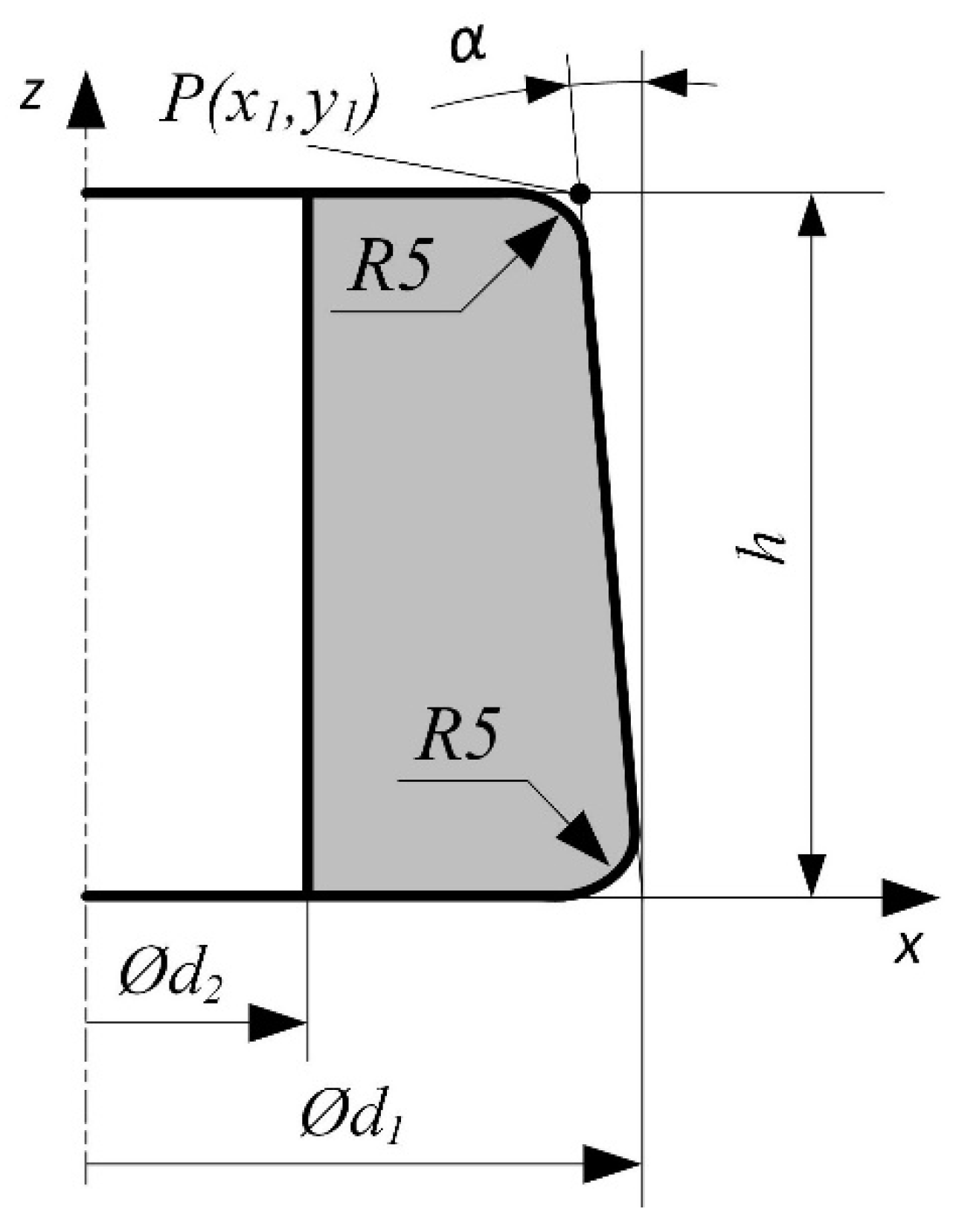
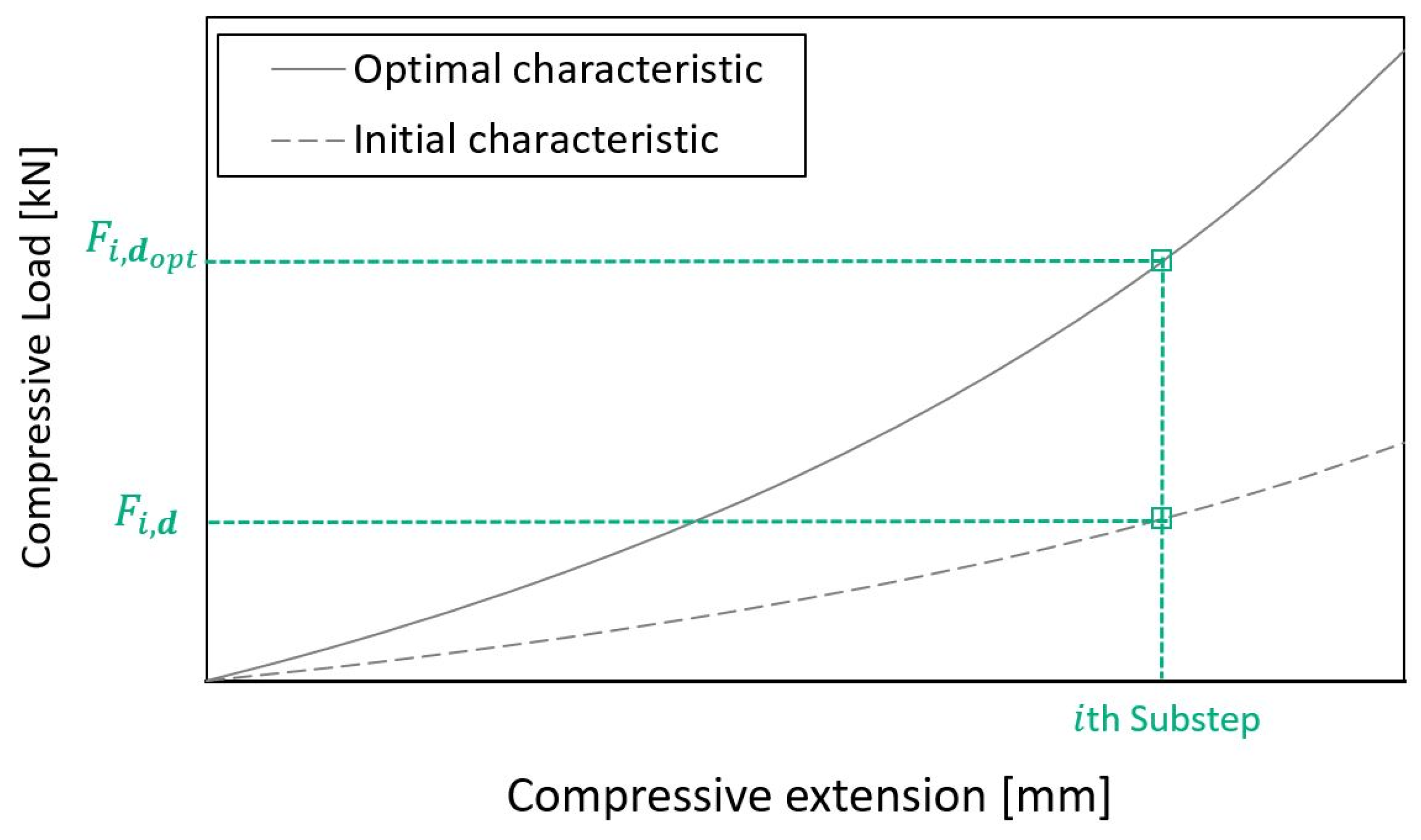
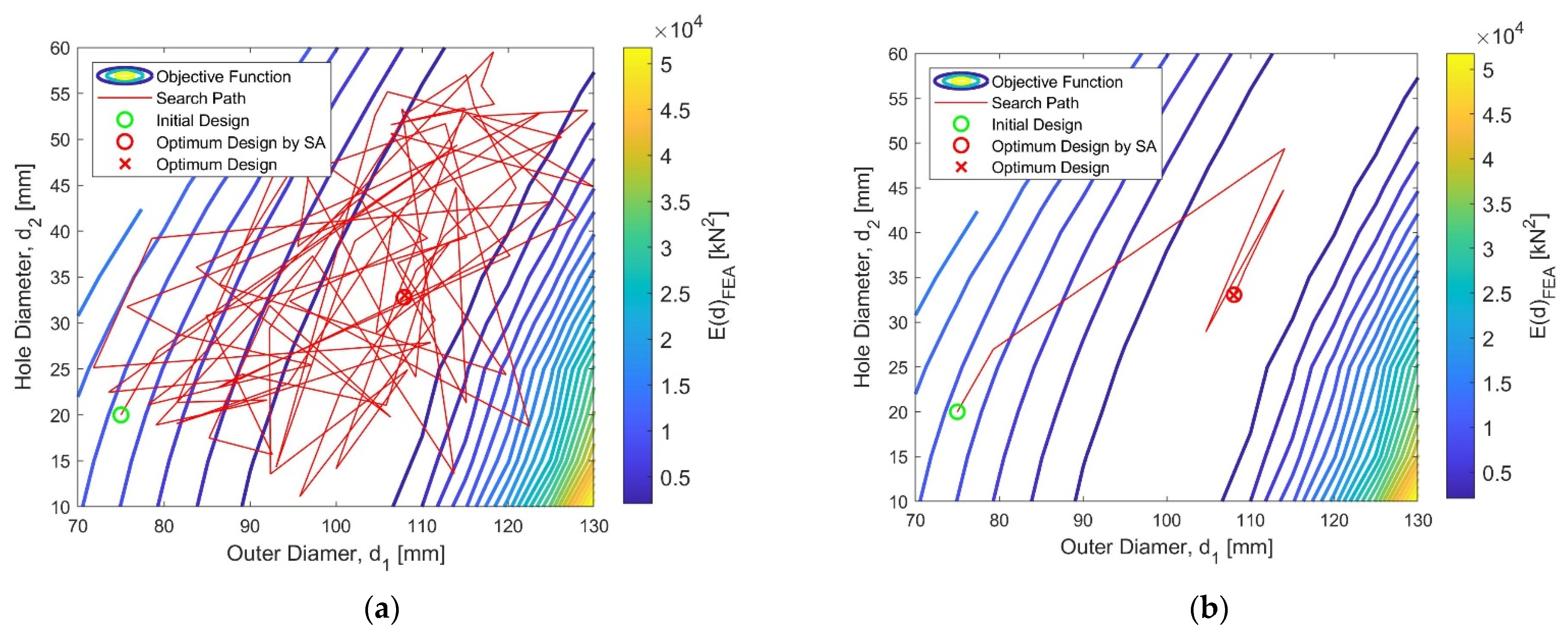
In this paper, the applicability of the method to be developed is demonstrated by solving a shape optimization problem of a rubber bumper built into air spring structures of lorries. One of the most important technical requirements for the investigated product is the force–displacement characteristics for a compressive load. By modifying the geometrical dimensions of the product, design engineers can achieve the desired working characteristics. This process is known as shape optimization. 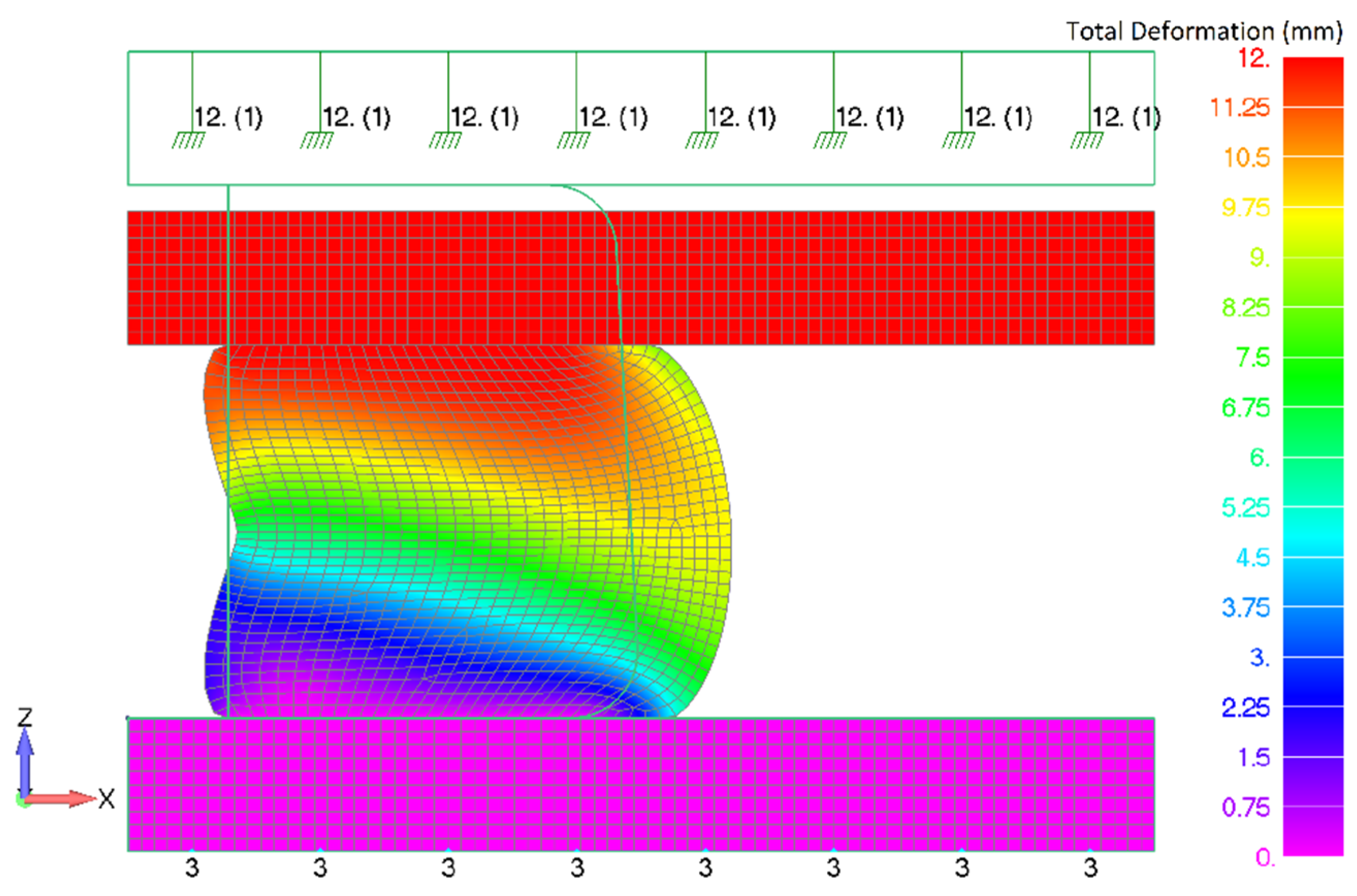Owing to the continuum mechanics background and hyperelastic material model available [1,2,3], trials can be carried out by applying finite element analysis. The rubber product can be simulated with a simplified model due to the axisymmetric geometric and boundary conditions, so the running time is not significant despite the nonlinear simulation.

Design optimization uses a mathematical formulation of a design problem to support the selection of the optimal design [4]. For the selection, the objective function is used, which is a scalar value formulated from a set of design responses; thus, it has different behaviors for a variety of problems. Several local and global search methods can be used if the computational cost of the optimization algorithm allows it to run on the model [5]. Because the gradient of the objective function calculated by finite element simulation is not given in the analytical form, but with approximate differences, gradient-based methods such as nonlinear programming by quadratic Lagrangian [6], mixed-integer sequential quadratic programming [7] or robust optimization [8] can be used to efficiently find the single global optimum. Direct methods, such as Powell’s method [9] and the Nelder–Mead simplex method [10,11], can approach the local minimum by using the value of the objective function. If limited information is available about the objective function behavior, it is recommended to use global optimal search methods. These include nature-inspired metaheuristic search methods such as the genetic algorithm [12], differential evolution [13] or simulated annealing (SA) which guarantees approaching the global optimum with the right settings. On the other hand, these algorithms require the selection of a number of parameters based on the task.

2. Literature Review

Several researchers have performed finite element simulation to successfully design rubber products, out of which [14,15,16,17,18,19] are the least efficient “trial and error” procedures. The combination of the finite element analysis with optimum search methods is more effective. A differential, evolution algorithm-based shape optimization of a rubber bushing was investigated by Kaya [20]. An engine mount using a parameter optimization method was designed by Kim [21], and Fletcher’s method applying the concept of quadratic convergence was used as the optimization algorithm. In MATLAB, environment particle swarm and gravitational search optimization methods were hybridized to solve a multiobjective optimization task for a volumetric compression restrainer device under earthquake excitation [22]. The shape optimization of fabric rubber seal used in aircraft doors was investigated in [23]. For the optimization task, a high number of design variables, several geometric and functional optimization constraints and a weighted multiobjective function were defined. For the pre-processing of the Abaqus finite element model, a developed Python script, for the search of the adaptive simulated annealing algorithm found in the Isight software and for the post-processing MATLAB software, was used. Despite the complex task, the search algorithm and the developed method proved to be effective for finding a better design.

If the calculation of the objective function is computationally expensive, it is preferable to use a surrogate model-based optimization method [24]. The aim is to explore the relation between the independent variables (input variables) and one or more dependent variables (response variables) with a lower calculation time. Different kinds of calculation efficient metamodels are known, such as the Kriging method, radial basis function, multivariable adaptive spline regression, neural networks, support vector regression (SVR) [25] or the response surface methodology (RSM), which is an integration of statistical and mathematical techniques [26]. The response surface generated by the genetic aggregation algorithm is the weighted combination of one or several metamodels out of full second-order polynomials, non-parametric regression, Kriging, and moving least squares; thus, it is a calculation demand solution [27,28,29]. Nevertheless, deep learning techniques require a huge amount of data and computational capacity; thus, they are not advised for simulation-based optimization tasks. The design of experiments (DOE) statistical technique is useful to obtain an optimal response [30]. DOE aims to determine how many and what kind of experiments have to be carried out optimally to obtain as much information as possible at the lowest cost [31]. 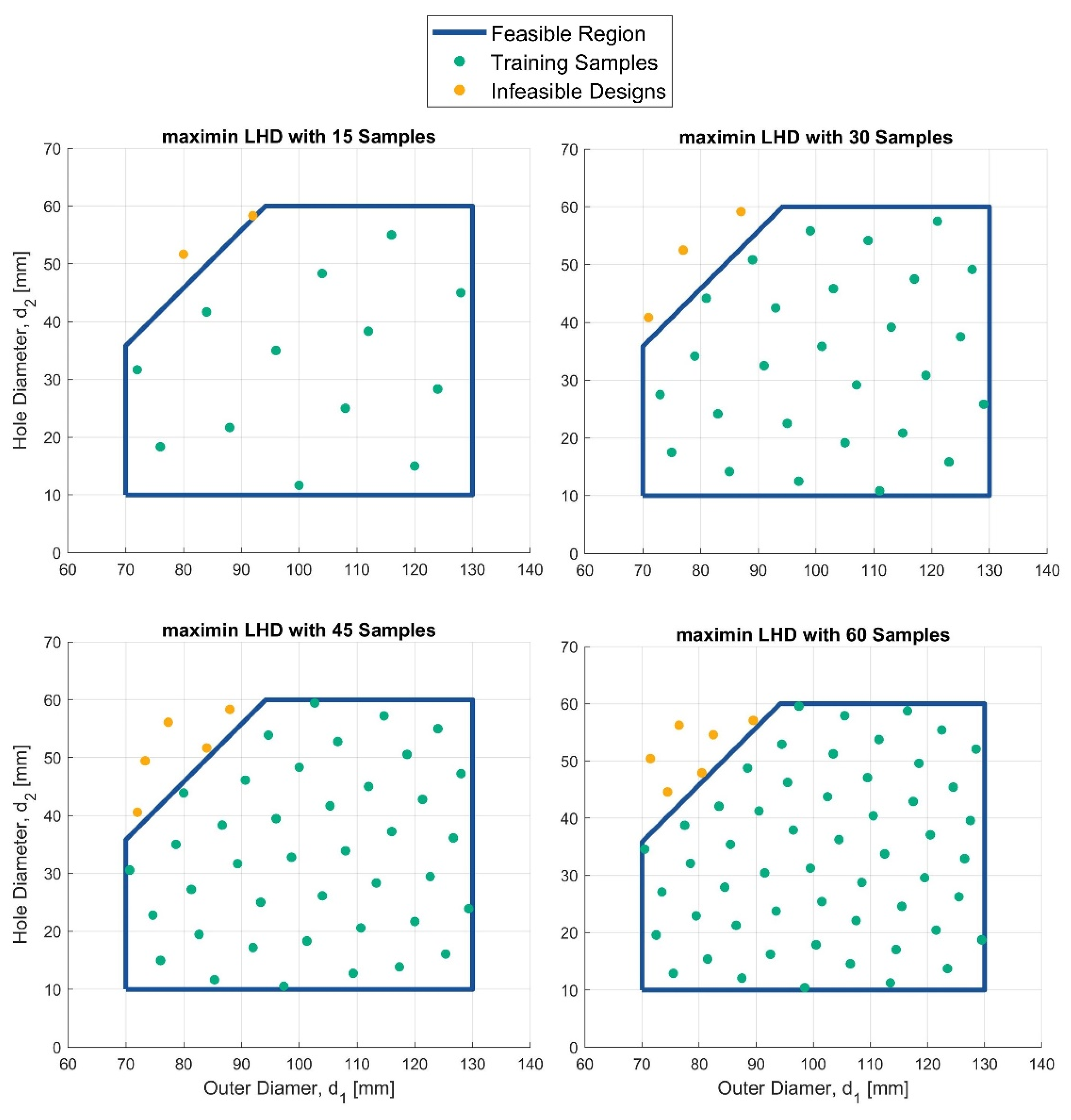Several experiment designs exist based on statistical criteria, such as the general full or fractional factorial design, central composite design (CCD) [26], the random and Latin hypercube design (LHD), Box–Behnken design [32], Taguchi design and other procedures (Montgomery, 2017) [33]. The selection of an LHD that maximizes the minimum distance among the points and was named the maximin LHD was introduced in [34]. Based on our previous research the response surface prediction precision fitted to the maximin Latin hypercube sampling method equals the tested CCD methods with identical sampling [35].

Metamodel-based design optimization was used for rubber product design using finite element simulation in some papers. The orthogonal experiment table was adopted to train the error backpropagation neural network model, which defines the nonlinear global mapping relationship between the geometric parameters of the rubber mount and its primary stiffness in the three principal directions [36]. The shape optimization task of rubber bumpers was investigated, where learning points were analyzed with finite element simulation. The SVR model was used to determine the given values of the objective functions of further constructions. Through a screening search algorithm, the optimal shape was determined [37]. Dynamic simulations and the Taguchi method using an orthogonal table were used to optimize a rotary control head rubber core sealing’s performance and fatigue life [38]. Support vector regression and random forest light-weight surrogate models were tuned to predict rubber suspension bushing stiffnesses for different load cases. The training dataset was selected using the DOE method based on 1D kernel density estimations, and the stiffnesses were calculated with finite element simulations [39]. Laboratory tests were performed with different axial loads on rubber bushes used in dynamic vibration absorbers and showed good agreement with the finite element analysis results. Thus, these methods were used to obtain a large number of samples for which the neural network surrogate model was trained in MATLAB to approximate the behavior of rubber bushes [40]. The cross-section of an automotive door sealing to reach a better door closing performance was optimized in [41]. The relation between the cross-section parameters and compression load deflection property was approximated with a neural network surrogate model. The efficiency of the genetic algorithm and particle swarm optimization methods was compared with the average of 50 runs. The different parameters of the genetic algorithm were tested on the neural network model. The found metamodel based optimum shape was compared with the finite element simulation results and showed a 7.9% relative error. Mankovits and Huri found the support vector regression model with cubic kernel function suitable to predict the new geometric construction of rubber bumpers [42,43].

Limited information is known in advance about the objective functions determined for the industry-related shape optimization tasks, so this paper uses simulated annealing for the search process. Another advantage of simulated annealing is that the search can be restarted from a new candidate point if there is an analysis running issue, which is common due to large deformations. Numerous new variants of the SA algorithm have been implemented in the last years to optimize engineering design problems [44,45,46,47]. In [48], two-dimensional structures subject to quasi-static loads were investigated using ANSYS, and the globally optimum shapes were obtained by the simulated annealing search algorithm. In [49], the shape optimization of a steel shear key using SA and Abaqus was run to enhance its cycle fatigue performance. Based on the aforementioned articles, the algorithms were able to find a good environment of the global optimum effectively if the algorithm parameters were preselected with a trial-and-error method that requires much human interaction. If there is sufficient time to run a simulated annealing algorithm, it will perform well with a slow cooling function and a high initial temperature, as shown by Anily and Federgruen [50]. However, a good solution has to be found by the searching algorithm in a short time when the cost function is calculated by expensive computer simulations. Therefore, numerous papers work on the parameter tuning of the simulated annealing algorithm considering the computational efficiency and accuracy [51,52]. The required number of function calls and the convergence speed of the algorithm highly depend on the treatment strategy of the temperature parameter, the effect of which has been examined in numerous research papers [53,54,55]. The values of annealing parameters for a given cooling strategy provide an additional option to reduce the computational cost of the algorithm as investigated in [56]. In [57] the annealing parameters were tuned analytically, while in [58] automatic parameter tuning using a genetic algorithm was studied. The appropriate choice of step size and initial temperature parameters was investigated for a wind turbine placement optimization task in [59]. Using the adaptive step size against the constant, the results were significantly improved. The adaptive simulated annealing algorithm developed by Ingber [60] uses an increasing number of parameters whose tuning process drastically enhances the complexity of the algorithm.

The accuracy of finite element simulations with a large deformation and hyperelastic material models is within the error limit of 5–10% accepted in engineering practice. The relative error can easily become unacceptable if additional uncertainty is expected in the design process, such as in the case of surrogate model-based optimization processes. Therefore, if enough time and computational capacity are available, the search procedure can run directly on the finite element model. The optimization methods used in the aforementioned articles were able to find a good solution from a technical aspect, but it has not been proved that the optimum found is the global one. None of the articles discussed how to automate the parameter tuning of algorithms while keeping accuracy and computational cost in mind. Therefore, the present work aims to develop a method suitable for such problems, specifically automating the algorithm tuning process for numerical simulation-driven design tasks. It also aims to shorten the time spent for testing and training the algorithm while increasing its robustness and eliminating the need for human interactions. A basic requirement for the algorithm is to approach the global optimum with enough precision to avoid increasing the modelling error. Another requirement is to estimate the number of iterations of the search algorithm so that computational resources and the time required for the optimization may be scheduled in advance.

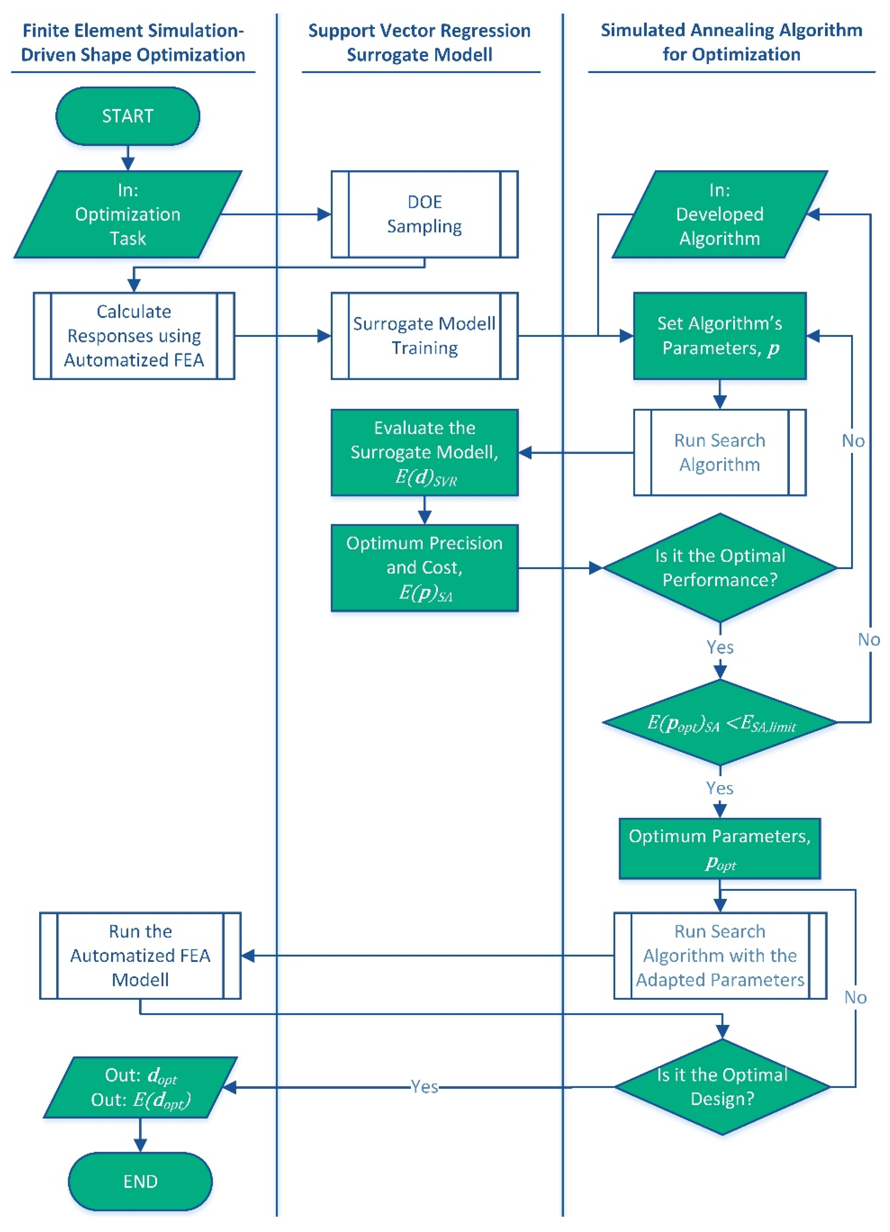
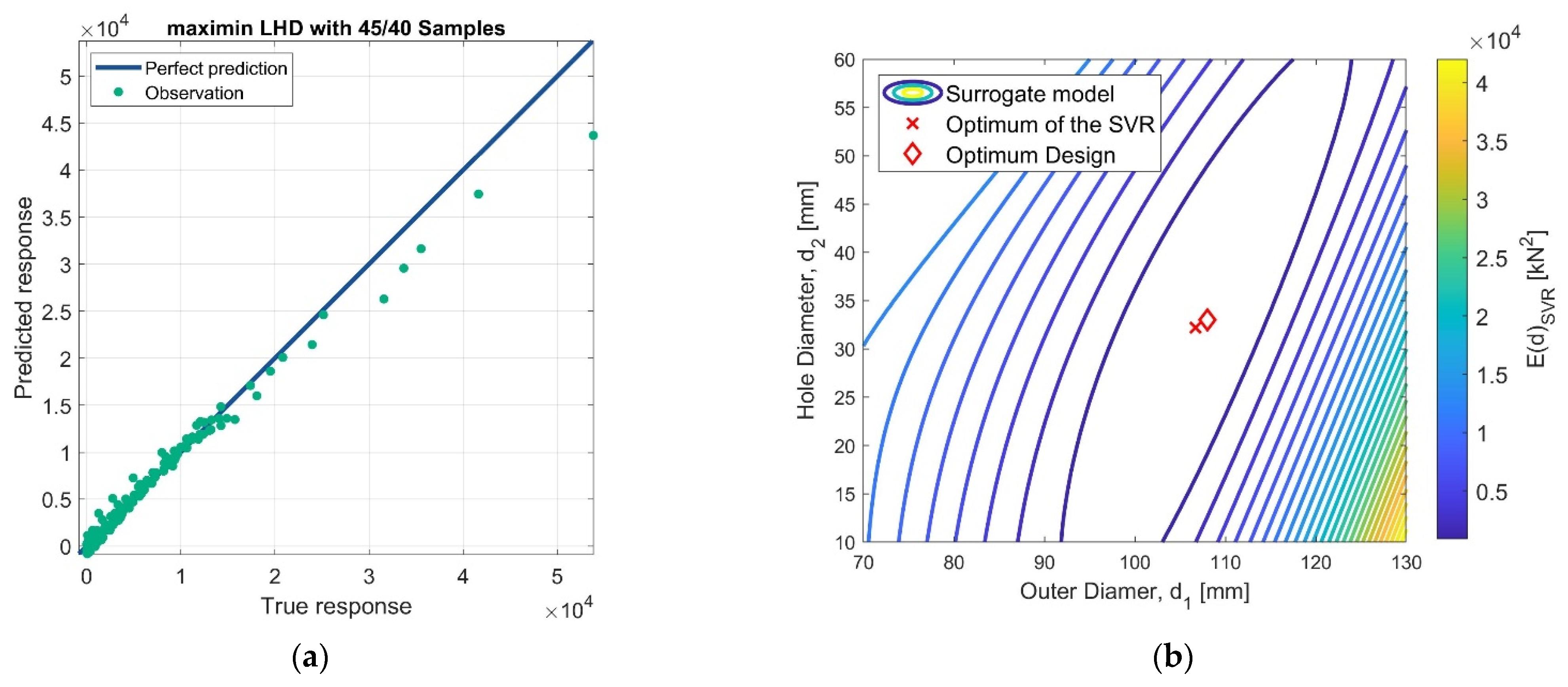
The novel approach is to perform the adaptation of the simulated annealing parameters while running on a surrogate model, which replaces the time-demanding numerical simulation-driven design process. The paper first introduces the developed method and the considerations that are necessary for the numerical simulation of the rubber product. In addition, because the task of the two-variable shape optimization of a rubber bumper is presented with the optimum known in advance, it can be used as a numerical optimization test function to evaluate the efficiency of the developed method. Using the optimal space-filling method, four datasets were prepared with different sample numbers to train the support vector regression surrogate model using the cubic kernel function. As an optimum search algorithm, a simulated annealing method with various cooling strategies was implemented in the MATLAB environment. The operation and robustness of the SA algorithm were tested by solving optimization test functions using the empirically obtained discrete parameter domain from the literature. Subsequently, the tuning of the SA parameters was performed by running the trained SVR surrogate model. Finally, the SA algorithm was used to perform the direct optimization of the finite element-based shape optimization problem with the previously determined parameter settings. Evaluating the results, the presented novel method proved to be accurate and efficient for the shape optimization of rubber bumpers. Due to its plannability and shorter design time, the method aids market competitiveness.

3. Model

3.1. Finite Element Simulation of the Rubber Bumper Working Characteristics

The investigated rubber bumper is used in the air springs of lorries, where after a certain decrease in height it works together with the air spring as a secondary spring. Due to its operational and manufacturing requirements, the height of the product is h $=40 \left[\mathrm{mm}\right]$ and the draft angle of the side is $\alpha =3°$, which can be seen in Figure 1. During its operation, the rubber bumper is subjected to a uniaxial compression between steel plates (Figure 2), up to a maximum of 30% of its height.

Different force–displacement curves, which characterize the technical behavior of the product, can be seen in Figure 3. In this particular case, the spring characteristics are optimized with the change of the outer diameter $d_1$ and the inner hole diameter $d_2$ variables of the cross-section; see in Figure 1.

The exact mixture of the styrene-butadiene rubber material of the investigated bumper is an industrial secret. Compression tests according to ISO 7743:2017 standard were performed up to $35\%$ strain on the base material to determine the stress–strain curve. It showed an incompressible nonlinear isotropic behavior, which can be modelled accurately with hyperelastic constitutive models such as the two-term Mooney–Rivlin [61], of which the strain energy function is

$$W_{MR}=c_{10}\left({\overline{I}}_1-3\right)+c_{01}\left({\overline{I}}_2-3\right)+\kappa {\left(J-1\right)}^2,$$

(1)

where ${\overline{I}}_1$ and ${\overline{I}}_2$ are the first and second strain invariants of the right Cauchy–Green tensor; $J$ is the Jacobian; and $c_{10}$, $c_{01}$ and $\kappa$ are material constants. In

Table 1. Defined attributes for the finite element discretization.

Element Type	Axisymmetric
element order, shape	linear four-node quadrilateral
element size	1 [mm]
material model	two-term Mooney–Rivlin
$\kappa$, bulk modulus	1000 [MPa]
$c_{10}$, material parameter	1.288 [MPa]
$c_{01}$, material parameter	1.137 [MPa]

, these material parameters were determined using the curve-fitting process, and the goodness of the fitted material model was compared with laboratory measurements [62,63].

The geometry and boundary conditions of the investigated rubber specimen are axisymmetric, thereby the geometry was discretized using the axisymmetric element type with attributes that can be seen in Table 1. Frictional contact pairs were defined between the rubber bumper and flat steel plates with self contact between the bore’s elements, where the ${\mu }_s=0.6$ coefficient of static friction was selected according to [64]. The lower steel plate displacement in the z-axis direction was constrained; furthermore, the upper steel plate has a 12 (mm) prescribed displacement in the negative z-axis direction.

The NX Nastran Advanced Nonlinear Static solver was used to deal with the nonlinearities derived from the material, contacts and large geometric changes. The finite element analysis was solved in 100 equally distributed substeps, and every 10th substep was created as the output. As a result, Figure 3 shows the load-displacement characteristics of the investigated product, while the operation of the constructed model and contacts can be observed through the deformation image seen in Figure 2.

3.2. Two-Dimensional Shape Optimization Problem

The current investigation aimed to achieve the optimal working characteristics by changing the shape of the product. The geometry of the product tested can be seen in Figure 1. Let $\Omega$ be the set of the $\mathit{d}$ vector of design variables, which is considered to be a continuous domain. Let the objective function be $E{\left(\Omega \right)}_{FEA}:{ℝ}^n\to ℝ$, the function which forms real numbers from set $\Omega \subseteq R^n$, and the relation can be determined by a finite element analysis of the rubber bumper compression test. The objective function is described as the difference between the initial and optimal working characteristics; see Figure 3. The aim is to decrease the value of the objective function during optimization by changing $\mathit{d}=\left(d_1,d_2\right)$. This means that the task of optimization is to find the minimum value of the objective function and determine a vector ${\mathit{d}}_{opt}$ describing the optimal shape

$$E{\left({\mathit{d}}_{opt}\right)}_{FEA}=\underset{\mathit{d}\in \Omega }{min}E{\left(\mathit{d}\right)}_{FEA}$$

(2)

subject to

$$\begin{array}{c}70\le d_1\le 130 \left[\mathrm{mm}\right]\\ 10\le d_2\le 60 \left[\mathrm{mm}\right]\\ x_1-d_2/2\ge 15\mathrm{where}{x}_1=d_1/2-\tan \left(\alpha \right)h\end{array}$$

(3)

and $x_1$ is the coordinate of point $P$, as seen in Figure 1. The equations describe the geometric optimization constraints and thus define the feasible region.

The difference between the initial and optimal working characteristics can be determined by calculating the sum of squared differences in the given points of the two working characteristics:

$$E{\left(\mathit{d}\right)}_{FEA}={\displaystyle \sum }_{i=10}^{100}{\left(F_{i,{\mathit{d}}_{opt}}-F_{i,\mathit{d}}\right)}^2$$

(4)

where $i\in \left\{10:10:100\right\}$, $E{\left(\mathit{d}\right)}_{FEA}$ is the error value in an investigated design point, and $F_{i,{\mathit{d}}_{opt}}$ is the optimal while $F_{i,\mathit{d}}$ is the investigated working characteristic-analysed compressive force value in the ith substep. $F_{i,\mathit{d}}$ is determined by evaluating the reaction force on the steel plate.

Table 2. Calculated cost function value in different design points.

	${\mathit{d}}_1 \left[\mathbf{m}\mathbf{m}\right]$	${\mathit{d}}_{2 }\left[\mathbf{m}\mathbf{m}\right]$	${\mathit{E}\left(\mathit{d}\right)}_{\mathit{F}\mathit{E}\mathit{A}} \left[\mathbf{k}{\mathbf{N}}^2\right]$
Optimum Shape, ${\mathit{d}}_{opt}$	108	33	0
Initial Shape, ${\mathit{d}}_{initial}$	75	20	9666

contains the calculated objective function value for the initial shape ${\mathit{d}}_{initial}=\left(75,20\right) \left[\mathrm{mm}\right]$.

The optimal characteristics were determined from the ${\mathit{d}}_{opt}=\left(108,33\right) \left[\mathrm{mm}\right]$ geometric shape known in advance, although this information will be only used for the conclusions. The introduced shape optimization problem will be used as a simulation-based optimization test function.

3.3. Test Dataset and the Objective Function Behavior

With the increment of $5 \left[\mathrm{mm}\right]$ along with the design variables, $128$ design points (DP) were selected from $\Omega$. With the use of the introduced finite element model of the rubber bumper, it is possible to calculate the $E{\left(\mathit{d}\right)}_{FEA}$ values for each sample point of the designs. To accelerate the finite element model pre- and post-processing, the parameterization of these processes is necessary. The automation of the whole process was feasible with the use of Femap Application Programming Interface (API). This is an object-oriented code written in the Visual Basic for Applications (VBA) language. This provided an opportunity to programmatically call the Femap functions for the finite element model pre- and postprocessing from Microsoft Visual Studio (VS) through the Component Object Model or Object Linking and Embedding (COM/OLE) interface. Using a Transmission Control Protocol (TCP), two-way communication was created between MATLAB and vs. to exchange data directly on a PC. As a result, it is feasible to control Femap functions via vs. from a MATLAB script containing the implementation of the sampling process, the later optimization task, and the search algorithm.

To generate the test dataset, the objective function value $E{\left(\mathit{d}\right)}_{FEA}$ was determined automatically for each number of samples. These data will be used later as an unknown sample to evaluate the performance of the fitted surrogate models. The objective function values are plotted above the test dataset, which is shaped like a valley (Figure 4). This behavior shows that convergence to the global optimum is not a trivial task.

4. Methods

4.1. Simulated Annealing Algorithm

Simulated annealing (SA) is a probabilistic metaheuristic search method for global optimization problems. It is mostly used for discrete optimization problems, although if an approximation of the optimum is good enough it can be used efficiently for continuous variables. The algorithm imitates the treatment strategy in metallurgy, of which the similarity and the name have been implemented by Kirkpatrick, Gelattt and Vecchi to solve combinatorial optimization problems [65]. There are numerous examples in the literature that summarize the theories of simulated annealing algorithms [66,67,68,69]. They contain four main components: the generation of the next candidate point, the acceptance function $P$, the cooling schedule $S$ and the stopping/convergence criterion $C$.

The algorithm uses the Metropolis criterion [70] to interpret the probability of accepting the cost-increasing function value, and this is where it differs from the hill climbing algorithm. Using the energy difference $\Delta E=E\left({\mathit{d}}_{\mathrm{new}}\right)-E\left({\mathit{d}}_k\right)$, the probability of making the transition to the new candidate design depends on the acceptance probability function $P_t$ calculated at $T_t$ temperature:

$$P_t\left({\mathit{d}}_k,{\mathit{d}}_{new},T_t\right)=\{\begin{array}{ccc}\hfill 1,& & if \Delta E<0\hfill \\ \hfill exp\left(\frac{-\Delta E}{T_t}\right),& & if \Delta E\ge 0\hfill \end{array}$$

(5)

At a lower energy state, the transition into the new candidate point will be accepted; otherwise, $P_t$ is its probability. At the beginning of the search, $T_t$ is high enough to allow the algorithm to make a transition out of any metastable state, although only the minimum energy state is accepted at a low value of the temperature [65].

4.2. Cooling Schedule

The major component of the algorithm is the cooling schedule $S\left(T_0,\Lambda ,N\right)$, which is defined by the selection of the initial temperature $T_0$, the cooling function $\Lambda \left(t\right)$ and the value of $N$ of trials per temperature. The selection of the cooling speed and the number of $N$ depend on each other; thus the latter parameter was selected empirically:

$$N=N_0·n$$

(6)

4.2.1. Initial Value of the Temperature Parameter

Let $\chi \left(T_t\right)$ denote the acceptance rate at a temperature $T_t$ which is defined by

$$\chi \left(T_t\right)=\frac{\mathrm{number}\mathrm{of}\mathrm{accepted}\mathrm{transitions}}{\mathrm{number}\mathrm{of}\mathrm{proposed}\mathrm{transitions}}.$$

(7)

As a general rule, when $T_t$ has a high value, all transitions are accepted using the Metropolis criterion; thus $\chi \left(T_t\right)$ is close to $1$. The selected initial value of temperature $T_0$ must be high enough to allow greater freedom in exploring the search space and to avoid sticking into the local minima. However, the too-high value of $T_0$ results in more function calls. There are several ways of determining the $T_0$ initial value of the temperature parameter, which must perform the requirement that virtually ($\chi \left(T_0\right)\ge 0.8$) all the proposed transitions should be accepted [65,71,72].

Let $m_t$ denote the number of trials at a $T_t$ temperature value, and $m_t=m_1+m_2$. The values of $m_1$ and $m_2$ correspond to the number of cost-decreasing and cost-increasing transitions, respectively, obtained. Furthermore, let ${\overline{\Delta E}}^{+}$ be the average value of the cost-increasing energy differences over the $m_2$ transitions. Then, the acceptance ratio $\chi \left(T_t\right)$ can be approximated as

$$\chi \left(T_t\right)\approx \frac{m_1+m_{2}exp\left(\frac{-{\overline{\Delta E}}^{+}}{T_t}\right)}{m_1+m_2}.$$

(8)

Thus, the initial value of the temperature $T_0$ can be calculated by the equation presented by Aarts and Van Leerhoven [73]

$$T_0\approx \frac{{\overline{\Delta E}}^{+}}{\ln \left(\frac{m_2}{m_2{\chi }_0-m_1\left(1-{\chi }_0\right)}\right)}$$

(9)

where ${\chi }_0=0.85$ is a commonly used value for the initial acceptance ratio. The domain of the logarithmic function is the set of positive real numbers; hence the $T_0$ can be calculated if the $m_0$ trials fulfil the following requirement:

$$m_2>m_0\left(1-{\chi }_0\right).$$

(10)

4.2.2. Cooling Functions

The convergence speed of the algorithm highly depends on the cooling function $\Lambda \left(t\right)$ of the $T$ temperature parameter, the effect of which was investigated in numerous research papers [53,54,55]. The algorithm requires generating a sequence of decreasing values of temperature $\mathit{T}=\left\{T_0,\dots ,T_t,\dots ,T_{min}\right\}$, which could be finite if the value of $T_{min}$ is given.

There are numerous temperature decreasing functions such as the exponential multiplication cooling, which was first proposed by Kirkpatrick, Gelatt and Vecchi [65]:

$$T_t=T_0{\mathsf{\alpha }}_1{}^t$$

(11)

where ${\mathsf{\alpha }}_1$ is the cooling speed parameter, which is a positive constant factor that lies between $0.8$ and $0.99$ [74]. A linear cooling function used by Randelman and Grest where $T_t$ is reduced with $\Delta T$ every $N$ trials [75]:

$$T_t=T_0-t\Delta T, \mathrm{and} T_t\ge T_{min}.$$

(12)

A fast simulated annealing method was introduced by Szu where the cooling schedule is inversely proportional to time [76]

$$T_t=\frac{T_0}{1+t}.$$

(13)

4.3. Generation of the Next Candidate Using Adaptive Step Size Control

To generate the ${\mathbf{\alpha }}_m$ step of the next candidate, normally distributed random numbers with zero mean and ${\rho }_{i,t}$ standard deviation are selected in all directions of the design variables. Selecting a too-small value for the step size ${\rho }_{i,t}$ the search can be stuck in local optima, while for too-large values the optimum can only be crudely approached. The initial step size ${\rho }_{i,0}$ was selected empirically based on the domain of the $i$-th design variable:

$${\rho }_{i,0}=\frac{\left(d_{i,max}-d_{i,min}\right)}{2}, i=1,\dots ,n.$$

(14)

The chance of the algorithm to find a better function value without narrowing the search space converges to zero. A 1/5 success rule was used by Schwefel to modify the step size of evolution-based searching strategies [77]. After every $N$ iteration, the search space was narrowed or increased based on the calculated value of the ${\chi }_{10N}$, which denotes the acceptance ratio for the last $10N$ iterations:

$${\chi }_{10N}={{\displaystyle \sum }}_{t-9}^{\mathrm{t}}\frac{\chi \left(T_t\right)}{10}.$$

(15)

Schewels’ rule was further investigated in [78], and a third case was defined where the step size was not modified:

$${\mathbf{\rho }}_{t+1}=\{\begin{array}{ccc}\hfill \min \left({\mathbf{\rho }}_0, {\mathbf{\rho }}_t/\beta \right),& & if {\chi }_{10N}>1-q\hfill \\ \hfill {\mathbf{\rho }}_t,& & if q\le {\chi }_{10N}\le 1-q\hfill \\ \hfill \beta {\mathbf{\rho }}_t,& & if {\chi }_{10N}<q\hfill \end{array}$$

(16)

where $q<0.5$ is the success rate, and $0<\beta <1$ is the step size adaptation factor.

4.4. Stopping and Convergence Criteria

The current section aims to define convergence criteria that is suitable for stopping the search sufficiently close to the optimum without knowing its values. Let $E\left({\mathit{d}}_k\right)$ be the $k$-th function value accepted by the Metropolis criterion, and its relative change compared to the $\left(k-1\right)$-th accepted step is

$$R{E}_{E\left({\mathit{d}}_k\right)}=\frac{\left|E\left({\mathit{d}}_k\right)-E\left({\mathit{d}}_{k-1}\right)\right|}{\left|E\left({\mathit{d}}_{k-1}\right)\right|}.$$

(17)

The step can be relatively small at any stage of the search process thanks to the stochastically generated new candidate, and thus the convergence condition can be met. The early stop can be avoided by averaging the absolute relative errors $\overline{RE}$ for the steps accepted in the last $m_C$ iteration. Let $\mathbf{\epsilon }=\left({\mathbf{\epsilon }}_{\mathit{d}},{\epsilon }_E\right)$ be the vector of the convergence tolerances with ${\mathbf{\epsilon }}_{\mathit{d}}$ representing the design variables limit, while ${\epsilon }_E$ represents the objective function limit. Thus, the condition for fulfilling the convergence criterion is

$$c{c}_1=1,\mathrm{if}{\overline{RE}}_{E\left({\mathit{d}}_k\right)}<{\epsilon }_E.$$

(18)

Let ${\mathit{d}}_k$ be the vector of the $k$-th accepted design variables, and its element relative change compared to the $\left(k-1\right)$-th accepted step is

$$R{E}_{d_{i,k}}=\frac{\left|d_{i,k}-d_{i,k-1}\right|}{\left|d_{i,k-1}\right|}, i=1,\dots ,n$$

(19)

Thus the condition for fulfilling the convergence criterion is

$$c{c}_2=1,\mathrm{if}{\overline{RE}}_{d_{i,k}}<{\epsilon }_{d,i} \mathrm{for}\mathrm{every} i=1,\dots ,n.$$

(20)

In the last case, when the maximum iteration number $m_{max}$ is reached, the process will be terminated by the stopping criterion

$$sc=1,\mathrm{if}m\ge m_{max}=3000·n.$$

(21)

Let $C\left(c{c}_1,c{c}_2,sc\right)$ denote the stopping/convergence criterion, which is activated if any of the previously mentioned conditions are met:

$$C\left(c{c}_1,c{c}_2,sc\right)=1,\mathrm{if} c{c}_1=1 \left|\left| c{c}_2=1 \right|\right| sc=1.$$

(22)

4.5. Pseudocode of the Simulated Annealing Algorithm

The simulated annealing algorithm with an adaptive step size control and different cooling strategies was implemented in a MATLAB environment using Algorithm 1, which was developed based on the aforementioned articles and Equations (5)–(22).

Algorithm 1: Simulated annealing algorithm with adaptive step size control
1.	(Initialization)
	Select an initial construction ${\mathit{d}}_0\in \Omega$; an initial temperature $T_0$; a number of trials per temperature $N$; a cooling function $\Lambda \left(t\right)$; an initial step size ${\mathbf{\rho }}_0$; a step size adaptation factor $\beta$; the parameters of the convergence criterion $m_C$ and $\mathbf{\epsilon }=\left({\mathbf{\epsilon }}_{\mathit{d}},{\epsilon }_E\right)$
	Set the counter of the objective function call $m=0$, the accepted moves $k=0$ and the cooling cycle $t=1$
	Set the variables of ${\mathit{d}}_k={\mathit{d}}_0$, ${\mathit{d}}_{opt}={\mathit{d}}_0$ ${\mathbf{\rho }}_t={\mathbf{\rho }}_0$, $T=T_0$
2.	(Generate a New Candidate)
	do generate a random step ${\mathit{a}}_m\left({\mathbf{\rho }}_t\right)\in {ℝ}^n$; ${\mathit{d}}_{m+1}={\mathit{d}}_k+{\mathit{a}}_m$
	while${\mathit{d}}_{m+1}\in \Omega$
	${\mathit{d}}_{new}={\mathit{d}}_{m+1}$$;\left(m=m+1\right)$
3.	(Metropolis Criterion)
	calculate $\Delta E=E\left({\mathit{d}}_{\mathit{new}}\right)-E\left({\mathit{d}}_k\right)$
	if$\Delta E<0$
	${\mathit{d}}_{k+1}={\mathit{d}}_{\mathit{new}}$$;\left(k=k+1\right)$
	if ${\mathit{d}}_{new}<{\mathit{d}}_{opt}$, ${\mathit{d}}_{opt}={\mathit{d}}_{\mathit{new}}$
	else generate a uniformly distributed random number $\left(r\right)$ in the interval $\left(0, 1\right)$
	if $r<P_t=exp\left(-\Delta E/T_t\right)$; ${\mathit{d}}_{k+1}={\mathit{d}}_{\mathit{new}}$, $\left(k=k+1\right)$
	end
4.	(Cooling Schedule, Step Size Adaptation)
	if$m\%N=0$
	$T_t\to T_{t+1}$, call the cooling function $\Lambda \left(t\right)$; Calculate ${\chi }_{10N}$; then $,{\mathbf{\rho }}_t\to {\mathbf{\rho }}_{t+1}$, call the adaptive step size control; $\left(t=t+1\right)$
	end
5.	(Stopping and Convergence Criteria)
	if$m>m_C$
	if $C\left(c{c}_1,c{c}_2,sc\right)=1$, check for stopping/convergence criterion
	stop the search with results ${\mathit{d}}_{opt}$, $E\left({\mathit{d}}_{opt}\right)$, $m$
	else go to step 2
	end
	end

4.6. Optimization Problem for the Parameter Adaptation of the Simulated Annealing Algorithm

The current investigation aims to tune the simulated annealing algorithm, which can efficiently find the global optimum. Let the objective function be $E{\left(\mathit{p}\right)}_{SA}:{ℝ}^n\to ℝ$, which is a measure of the cost and precision of the algorithm:

$$E{\left(\mathit{p}\right)}_{SA}=w_{1}E{\left(\mathit{p}\right)}_{SA, succ}+w_{2}E{\left(\mathit{p}\right)}_{SA, cost},$$

(23)

where $E{\left(\mathit{p}\right)}_{SA, succ}$ is the success of the found optimum, $E{\left(\mathit{p}\right)}_{SA, cost}$ is the computational cost, while $w_1$ and $w_2$ are weighting factors. In this particular case, $w_1=10$ and $w_2=1$. The $E{\left(\mathit{p}\right)}_{SA,succ}$ depends on the $f_{opt,SA}$ found by the algorithm and the specified in advance $f_{limit}$ objective function value:

$$E{\left(\mathit{p}\right)}_{SA, succ}=\{\begin{array}{c}\begin{array}{ccc}0\hfill & & ,\mathrm{if} f_{opt,SA}<f_{limit}\hfill \end{array}\\ \begin{array}{ccc}1\hfill & & ,\mathrm{if} f_{opt,SA}\ge f_{limit}\hfill \end{array}\end{array}$$

(24)

The algorithm can only converge after the $m_C$ iteration, in which case the $E{\left(\mathit{p}\right)}_{SA, cost}=0$, whereas the $E{\left(\mathit{p}\right)}_{SA, cost}=1$ if it stops at the maximum iteration $m_{max}$, in other cases taking a proportional value

$$E{\left(\mathit{p}\right)}_{SA, cost}=\frac{m-m_c}{m_{max}-m_c}.$$

(25)

Due to the stochastic search, running the algorithm with the same parameters results in a deviation in the number of iterations and the found optimum, as well as the value of the $E{\left(\mathit{p}\right)}_{SA}$ objective function. Therefore, the parameters of the algorithm were chosen from the literature’s empirically obtained discrete parameter domain. Out of all the possible parameter combinations, the goal is to find the one that performs the best. Let $\Psi$ be the set of $\mathit{p}=\left(p_1,p_2,p_3\right)$ vectors of the SA algorithm variable parameters, which is considered to be a discrete domain. The task of optimization is to find the minimum value of the objective function and determine a vector ${\mathit{p}}_{opt}$ describing the optimal parameter setting

$$E{\left({\mathit{p}}_{opt}\right)}_{SA}=\underset{\mathit{p}\in \Psi }{\min }E{\left(\mathit{p}\right)}_{SA}$$

(26)

subject to

$$\begin{array}{c}{p}_1=\beta \in \left\{0.625:0.075:0.925\right\}\\ p_2=\Lambda \in \left\{1,2,3\right\}\\ \begin{array}{c}{p}_3={\mathsf{\alpha }}_1\in \left\{0.7:0.05:0.95\right\} \left|\right| {\mathsf{\alpha }}_2\in \left\{1,4,8,16,32,64\right\}\\ E{\left({\mathit{p}}_{opt}\right)}_{SA}\le E_{SA,limit}=1\end{array}\end{array}$$

(27)

where $\beta$ is the step size adaptation factor, ${\mathsf{\alpha }}_1$ is the cooling speed parameter, ${\mathsf{\alpha }}_2$ is the linear cooling speed parameter, $E_{SA,limit}$ is the worst acceptable objective function value and $\Lambda$ is the cooling function:

$$\Lambda =\{\begin{array}{ccc}1,\hfill & & \mathrm{where} T_t=T_0{\mathsf{\alpha }}_1{}^t\hfill \\ 2,\hfill & & \mathrm{where} T_t=max\left(T_0-t\Delta T, T_{min}\right)\hfill \\ 3,\hfill & & \mathrm{where} T_t=T_0/\left(1+t\right)\hfill \end{array}$$

(28)

where $T_0$ is the initial temperature, $T_{min}=0.001$ and $\Delta T$ is the amount of temperature reduction:

$$\Delta T={\mathsf{\alpha }}_2\Delta T_{min}={\mathsf{\alpha }}_2\frac{\left(T_0-T_{min}\right)N}{m_{max}},\mathrm{where} 1\le {\mathsf{\alpha }}_2.$$

(29)

4.7. Introduction of the Surrogate Model-Based Parameter Tuning of Optimization Algorithm Method for Computationally Intensive Engineering Simulations

The current investigation aims to develop a novel method for the adaptation of simulated annealing parameters, which occurs in computationally intensive simulation-based optimization tasks. The optimization task seen in Section 4.6 takes 65 runs, which itself is a calculation- and time-demanding task thanks to the finite element analysis. Because of the metaheuristics of the algorithm, the value of the objective function $E{\left(\mathit{p}\right)}_{SA}$ can only be evaluated by taking the mean value of multiple calculations, meaning the task takes an unreasonable amount of time. The main idea of the research is to test the algorithm while running on a surrogate model, which is replacing the time-demanding simulation process. With the tuned parameter setting ${\mathit{p}}_{opt}$, it is assumed that the simulated annealing algorithm can approach the optimum of the shape optimization problem with a predictable function call. The flowchart of the developed surrogate model-based parameter tuning process of the optimization algorithm can be seen in Figure 5.

5. Results and Discussion

5.1. Design of Experiment to Generate Train Data Set

The precision of the surrogate model approaching the objective function to be applied largely depends on the number of design points and the distribution in the design area. Three-level sampling is required to describe the nonlinear behavior of the rubber material and the objective function. Sampling methods such as face-centered composite design or the three-level full factorial design are not usable in this particular task because of the optimization constrain between the design variables. When the numerical simulation contains few design variables, the Latin hypercube method is a good solution. By using this method, the number of the samples can be freely chosen, and the experiment level is identical to the number of samples. There are several sampling methods available within this particular method; in the current case, the maximin Latin hypercube was selected [34]. Taking the lower and upper limits of the design variables into account, 15, 30, 45 and 60 samples were selected. Afterwards, points are deleted that do not match the geometrical constrain set by (3). Thus, the training data sets contain 13, 27, 40 and 54 samples, the distribution of which can be seen in Figure 6.

5.2. Train Support Vector Regression Model

The objective of the surrogate modelling technique is to discover a function $E{\left(\mathit{d}\right)}_{SVR}\approx E{\left(\mathit{d}\right)}_{FEA}$ that best predicts the value of $E{\left(\mathit{d}\right)}_{FEA}$ associated with each value of $\mathit{d}$. The investigated shape optimization task is a nonlinear regression problem for which supervised machine learning methods could provide an efficient way to handle it. For data regression, support vector regression (ε-SVR) was introduced in [25], which uses the so-called kernel trick [79] to transform the original nonlinear input data to a higher-dimensional kernel space, where the relation between the inputs and response can be linearly estimated. The goodness of the prediction highly hinges on the kernel function type, which was investigated by us in [32], and the cubic kernel function proved to be the best choice.

With the use of the training dataset sampled by maximin LHD and the Regression Learner application built into MATLAB, it is possible to tune automatically the hyperparameters of the ε-SVR model. For small datasets, the usage of the k-fold cross-validation method is recommended to analyze the model fitting error. The investigation of Kohavi suggests that $k=10$ is the optimal value for a general task [80]. The tuning process of the ε-SVR model was performed for the different sets of training samples, and the root mean square error (RMSE) was calculated for the test dataset (128 DP) seen in

Table 3. Comparison of the performance of the support vector regression models with cubic kernel functions for different sets of samples using the root mean square error.

Kernel Function	Cross- Validation	RMSE
		S 15/13	S 30/27	S 45/40	S 60/54
Cubic SVM	10-fold	1927.45	1630.38	1411.24	1478.19

. The results showed that the training dataset with the increasing number of samples improved the accuracy of the SVR model. However, after the 45/40 training dataset, there was no further improvement in the accuracy. Therefore, the SVR models tuned with 40 samples and the cubic kernel function will be used in the later processes.

The predicted response $E{\left(\mathit{d}\right)}_{SVR}$ of the cubic SVR model is plotted against the true response $E{\left(\mathit{d}\right)}_{FEA}$; see Figure 7a. A perfect regression model has a predicted response equal to the true response, so all the points lie on the diagonal line. The vertical distance from the line to any point is the error of the prediction for that point. The selected SVR model predictions are scattered near the diagonal line, which means that the SVR model accurately predicts the nonlinear objective function values.

Using the trained cubic SVR model, predictions were made for each combination of integer values of design variables. Predicted objective function values are illustrated above the design space according to Figure 4. As a result, it seemed suitable for approaching the values of the nonlinear objective function. The SVR model isoline visualization, which shows valley-shaped behavior similar to the original function, can be seen in Figure 7b.

5.3. Testing the Tuning Process of the Simulated Annealing Algorithm for Mathematical Test Functions

Multimodal and valley characteristics are common properties of the objective function prescribed for the optimization task. Thus, the Rosenbrock, six-hump camel, McCormick and Michalewicz optimization problems were selected according to

Table 4. Mathematical optimization test functions.

Test Function	Variable Domain		${\mathit{x}}_{\mathit{o}\mathit{p}\mathit{t}}$	${\mathit{f}}_{\mathit{o}\mathit{p}\mathit{t}}$	${\mathit{f}}_{\mathit{l}\mathit{i}\mathit{m}\mathit{i}\mathit{t}}$
Rosenbrock	$x_1\in \left[-5,10\right]$	$x_2\in \left[-5,10\right]$	$\left(1,1\right)$	$0$	$0.01$
Michalewicz	$x_1\in \left[0,\pi \right]$	$x_2\in \left[0,\pi \right]$	$\left(2.20,1.57\right)$	$-1.8013$	$-1.8$
Six-hump camel	$x_1\in \left[-3,3\right]$	$x_2\in \left[-2,2\right]$	$\left(0.0898,-0.7126\right)$ $\left(-0.0898,0.7126\right)$	$-1.0316$	$-1.03$
McCormick	$x_1\in \left[-1.5,4\right]$	$x_2\in \left[-3,4\right]$	$\left(-0.54719,-1.54719\right)$	$-1.9133$	$-1.91$

to test the algorithm and its parameter optimization tasks.

The optimization task (objective function, design parameters, design variables and design constraints) and the simulated annealing algorithm were implemented in MATLAB script. To increase the robustness of the SA method, the algorithm was run numerous times using 100 pieces of randomly selected initial designs, and so the average value of the $\overline{E}{\left(\mathit{p}\right)}_{SA}$ was determined.

Table 5. Parameters of the simulated annealing algorithm for the different test functions.

Test Function	Initial Temperature		Step Size Adaptation			Convergence
	${\mathit{m}}_0$	$\mathit{\chi }\left({\mathit{T}}_0\right)$	${\mathit{\rho }}_0$	$\mathit{N}$	$\mathit{q}$	$\mathit{\epsilon }$	${\mathit{m}}_{\mathit{C}}$	${\mathit{m}}_{\mathit{m}\mathit{a}\mathit{x}}$
Rosenbrock	$100$	$0.85$	$\left[7.5,7.5\right]$	$20$	$0.2$	$\left[0.1,0.1,0.001\right]$	$100$	$6000$
Michalewicz	$100$	$0.85$	$\left[\pi /2,\pi /2\right]$	$20$	$0.2$	$\left[0.1,0.1,0.001\right]$	$100$	$6000$
Six-hump camel	$100$	$0.85$	$\left[3,2\right]$	$20$	$0.2$	$\left[0.1,0.1,0.001\right]$	$100$	$6000$
McCormick	$100$	$0.85$	$\left[3.25,3.5\right]$	$20$	$0.2$	$\left[0.1,0.1,0.001\right]$	$100$	$6000$

shows the empirically selected parameters of the algorithm based on the reviewed literature. Using the selected initial designs and (9), the average value of the initial temperature was calculated analytically. The step size $\mathbf{\rho }$ was adaptive during the search process following the method seen in (16), while the initial value ${\mathbf{\rho }}_0$ was determined using (14). The cooling function and the step size adaptation factor $\beta$ have the most impact on the computational cost and accuracy of the algorithm, so these parameters are the variables of the optimization task (26)–(29).

The simulated annealing algorithm was run for a finite number of discrete parameter combinations on different test functions. The best-performing parameters were selected from the results, shown in

Table 6. Optimal parameter settings for different mathematical test functions.

Test Function	$\overline{\mathit{E}}{\left({\mathit{p}}_{\mathit{o}\mathit{p}\mathit{t}}\right)}_{\mathit{S}\mathit{A}}$	Repeatability		$\mathit{S}\left({\mathit{T}}_0,\mathit{\Lambda },\mathit{N}\right)$, Annealing Schedule				$\mathit{\beta }$, Step Size Adaptation Factor
		Mean	SD	Λ, Cooling Function	${\mathsf{\alpha }}_1,$ Cooling sp.	${\mathsf{\alpha }}_2$, Linear Cooling sp.	${\mathit{T}}_0$, Initial Temp.
Rosenbrock	0.74659	0.9291	0.27690	1	0.70	-	436,335	0.925
Michalewicz	0.07565	0.0752	0.00023	1	0.70	-	1.065	0.625
Six-hump camel	0.14214	0.1426	0.00045	1	0.70	-	72.731	0.625
McCormick	0.12670	0.1274	0.00040	1	0.70	-	26.894	0.625

. Using these parameters, the test was performed 20 times to analyze the repeatability of the $\overline{E}{\left({\mathit{p}}_{opt}\right)}_{SA}$ average objective function value. For all mathematical test functions, the exponential cooling function with a fast cooling speed proved to be the best option. Unlike the other test functions, in the case of the Rosenbrock, the slow search space narrowing seemed to be effective. The deviation of the $\overline{E}{\left({\mathit{p}}_{opt}\right)}_{SA}$, which is derived from the success deviation, shows how difficult is for the algorithm to approach the Rosenbrock’s optimum. Despite this, the found $f_{opt}$ for the Rosenbrock is more than 95% accurate. However, despite the stochastic behavior, the parameter tuning method worked well based on the repeatability of the $\overline{E}{\left({\mathit{p}}_{opt}\right)}_{SA}$ for the other test functions. This proves that the developed convergence criterion is correct.

5.4. Tuning Simulated Annealing Algorithm for Shape Optimization

To terminate the SA algorithm with a high probability near the global optimum, the cooling strategy must be chosen case-by-case for the shape optimization task. While the accuracy of the optimum approach is affected by the step size adaptation factor, $\beta$. This parameter also greatly affects the number of function evaluations of the algorithm, which results in an increased length for the simulation-based design process. Thus, the determination of the optimal parameters was performed by running the trained SVR surrogate model, following the method used on the test functions. The dimensional tolerances of the rubber product were $\pm 0.1 \left[\mathrm{mm}\right]$; thus, the $f_{limit}$ value was determined (see

Table 7. The found optimum of the fitted SVR metamodel for the discrete variable domain.

Objective Function	${\mathit{d}}_{\mathit{l}\mathit{i}\mathit{m}\mathit{i}\mathit{t}}\left[\mathbf{m}\mathbf{m}\right]$	${\mathit{f}}_{\mathit{l}\mathit{i}\mathit{m}\mathit{i}\mathit{t}}\left[\mathbf{k}{\mathbf{N}}^2\right]$
Cubic SVR	$\left(106.7,32.2\right)$	$-840.487$

) on the following discrete domain:

$$f_{limit}=\underset{\mathit{d}\in \Omega }{\min } E{\left(\mathit{d}\right)}_{SVR},$$

(30)

subject to

$$\begin{array}{c}{d}_1\in \left\{70:0.1:130\right\} \left[\mathrm{mm}\right]\\ d_2\in \left\{10:0.1:60\right\} \left[\mathrm{mm}\right]\\ x_1-d_2/2\ge 15\mathrm{where}{x}_1=d_1/2-d_3\tan \left(d_4\right)\end{array}$$

(31)

The constant parameters were chosen empirically according to

Table 8. Parameters of the simulated annealing algorithm for the shape optimization.

Initial Temperature		Step Size Adaptation			Convergence
${\mathit{m}}_0$	$\mathbf{\chi }\left({\mathit{T}}_0\right)$	${\mathbf{\rho }}_0$	$\mathit{N}$	$\mathit{q}$	$\mathbf{\epsilon }$	${\mathit{m}}_{\mathit{C}}$	${\mathit{m}}_{\mathit{max}}$
$100$	$0.85$	$\left[30,25\right]$	$20$	$0.2$	$\left[0.1,0.1,0.001\right]$	$100$	$6000$

, and then the parameters of the simulated annealing algorithm were tuned.

Table 9. Tuned SA parameters for the SVR surrogate model.

Surrogate Model	$\overline{\mathit{E}}{\left({\mathit{p}}_{\mathit{o}\mathit{p}\mathit{t}}\right)}_{\mathit{S}\mathit{A}}$	Repeatability		$\mathit{S}\left({\mathit{T}}_0,\mathit{\Lambda },\mathit{N}\right)$, Annealing Schedule				$\mathit{\beta }$, Step Size Adaptation Factor
		Mean	SD	Λ, Cooling Function	${\mathsf{\alpha }}_1,$ Cooling sp.	${\mathsf{\alpha }}_2$, Linear Cooling sp.	$T_0$, Initial Temp.
Cubic SVR	0.07787	0.07811	0.00032	2	-	64	20430	0.625

shows the settings that performed the best on the SVR surrogate model.

5.5. Shape Optimization of the Rubber Bumper Using the Tuned Simulated Annealing Algorithm

The current section aims to evaluate the performance of the SA algorithm with the SVR tuned parameter setting by solving the finite element-based shape optimization problem directly. The search was repeated 11 times from the initial design ${\mathit{d}}_{initial}$.

Table 10. The optimal design variables found by the simulated annealing algorithm.

Design Point	${\mathit{d}}_1\left[\mathbf{m}\mathbf{m}\right]$	${\mathit{d}}_2\left[\mathbf{m}\mathbf{m}\right]$	$\mathit{E}{\left(\mathit{d}\right)}_{\mathit{F}\mathit{E}\mathit{A}}\left[\mathbf{k}{\mathbf{N}}^2\right]$
${\mathit{d}}_{initial}$	75	20	9666.118
${\mathit{d}}_{opt}$	108	33	0
${\mathit{d}}_{opt, SA}$	108.034	33.071	0.00005

shows the found ${\mathit{d}}_{opt, SA}$ optimal construction relating to the median $E{\left({\mathit{p}}_{opt}\right)}_{SA}$ value run. The algorithm approached the known optimal construction ${\mathit{d}}_{opt}$ within the dimensional tolerances of the rubber product, meaning that the optimum variables’ value ${\mathit{d}}_{opt, SA}$ is accurate from a technical point of view.

The working characteristic found by the tuned SA algorithm can be seen in Figure 8. It approaches the desired compressive force values within a 0.1% relative error, as seen in

Table 11. The working characteristic found by the tuned SA algorithm and its relative error when compared to the desired characteristic.

	Compressive Extension [mm]
	1.2	2.4	3.6	4.8	6	7.2	8.4	9.6	10.8	12
$F_{i,{\mathit{d}}_{opt}}\left[N\right]$	4805	10,266	16,424	23,445	31,462	40,627	51,226	63,479	77,933	95,028
$F_{i,{\mathit{d}}_{opt,SA}}\left[N\right]$	4805	10,267	16,426	23,447	31,464	40,629	51,228	63,480	77,932	95,024
$RE[\%]$	0.013	0.012	0.010	0.009	0.007	0.006	0.003	0.001	−0.002	−0.005

.

Figure 9a shows the search path taken by the SA algorithm. Using the initial temperature value calculated on the SVR model, the Metropolis criterion also accepts cost-increasing function values at the beginning of the search process.

On the surrogate model, the number of iterations $m$ was estimated to have less than 5% relative error; see

Table 12. Accuracy of the number of iterations and initial temperature determined by the run of the SVR model against the FEA.

Objective Function	$\overline{\mathit{E}}{\left({\mathit{p}}_{\mathit{o}\mathit{p}\mathit{t}}\right)}_{\mathit{S}\mathit{A}}$	SD of $\overline{\mathit{E}}{\left({\mathit{p}}_{\mathit{o}\mathit{p}\mathit{t}}\right)}_{\mathit{S}\mathit{A}}$	$\overline{{\mathit{T}}_0}$	$\overline{\mathit{m}}$
Cubic SVR	0.07811	0.00032	20,430	561
Rubber FEA	0.08071	0.00145	20,367	576
$RE[\%]$	−3.221	-	0.308	−2.662

. Running the finite element model, the average initial temperature $\overline{T_0}$ was calculated using (9) and the 100 pieces of randomly selected initial designs. This process requires the evaluation of ${10}^4$ objective functions, which would take days calling the finite element model, while only minutes in the case of the SVR surrogate model. However, as seen in Table 12, the initial temperature values determined by the run of the SVR and FEA models differ only slightly.

6. Conclusions

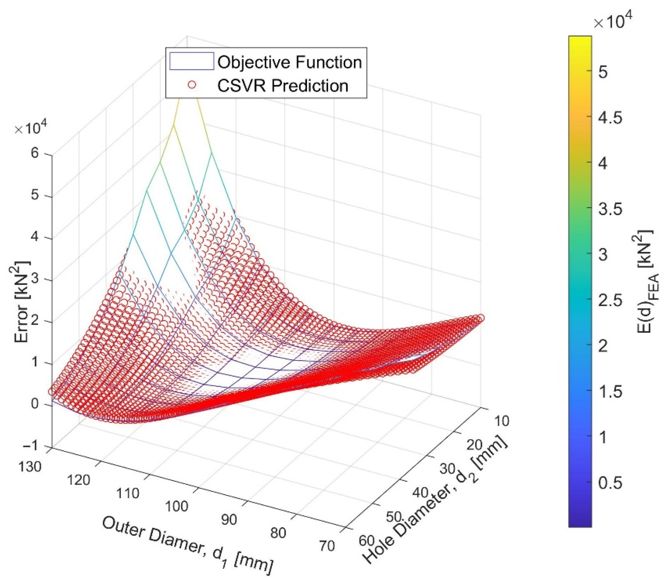
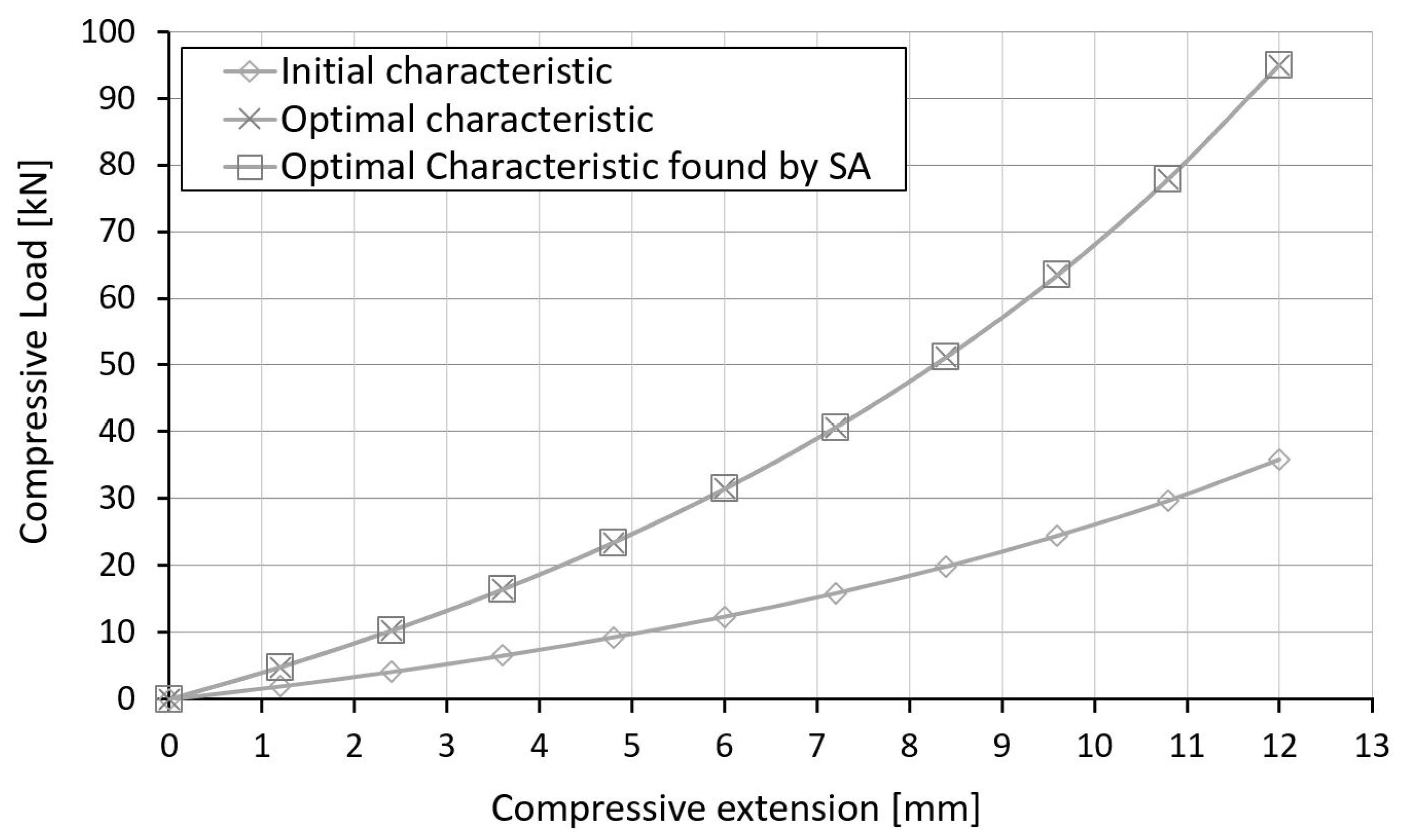
Foremost, a finite element simulation-based two-dimensional shape optimization problem was introduced. The objective function was determined as the difference between the initial and the optimum characteristic and showed a valley-shaped behavior, which is itself a challenging task for a search algorithm. A simulated annealing algorithm with an adaptive search space and different cooling schedules was implemented in a MATLAB environment. Because of the time-consuming objective function call and the stochastic behavior of the SA algorithm, the parameter tuning process is infeasible with the direct call of the finite element simulation task. To solve the tuning process, a novel procedure was introduced using an SVR surrogate model to test the optimization algorithm performance case-specifically. Sampling took place by means of the maximin Latin hypercube design method to perform the SVR training, where the dataset of 40 samples proved to be suitable to surrogate the two-dimensional shape optimization task of the rubber product.

The operation and robustness of the SA algorithm were tested by solving optimization test functions. The best performing parameters can be selected task-specifically using the empirically obtained discrete parameter domain from the literature. The optimum value is unknown by the algorithm, but it was able to approach it during the optimization of the mathematical test functions and the shape optimization task. This proves that the developed algorithm and its convergence criterion were correct. The tuned SA algorithm found an optimal design with negligible error from a technical aspect, thereby not increasing further the modelling errors due to nonlinear material behavior and large deformation.

Each step of the metamodel-based parameter tuning of the optimization algorithm can be automated, thus eliminating the need for engineering intervention in simulation-based design processes. The developed method enables the prediction of the development lead time in simulation-driven optimization processes. In terms of precision and number of function runs required for optimum determination, the tuned SA algorithm proved to be efficient. The determination of the initial temperature on the surrogate model is accurate and saves a significant amount of time. Regardless of the complexity of the simulation task, the time required for the developed method is solely determined by the computation time of the surrogate model. The method aids market competitiveness due to the plannability and shorter design time.

The newly introduced method opens up a slew of new research possibilities. One area is the large scale optimization problem for which the SVR surrogate model and SA algorithm are suitable methods. The surrogate model and optimization algorithm can be freely chosen in the developed parameter tuning process, allowing for the development of new methods as well as the assessment of their efficiency. Another extension of the developed method could be to perform a surrogate model-based parameter tuning of various global search algorithms to choose the best performer. In the future, the impact of the $T_0$ initial temperature of the SA can be investigated. The developed method is suitable for solving not only numerical simulation optimization problems but also for other computationally intensive model-driven optimizations.

References

1. El Yaagoubi, M.; Fulari, G.S.; Aloui, S.; Shetty, R.R. Influence of Permanent Deformation on the Fitting Quality and the Simulation Prediction of Filled Elastomers. Int. J. Non. Linear. Mech. 2021, 137, 103801. [Google Scholar] [CrossRef]
2. Nguyen, H.-D.; Huang, S.-C. The Uniaxial Stress–Strain Relationship of Hyperelastic Material Models of Rubber Cracks in the Platens of Papermaking Machines Based on Nonlinear Strain and Stress Measurements with the Finite Element Method. Materials 2021, 14, 7534. [Google Scholar] [CrossRef] [PubMed]
3. Aloui, S.; El Yaagoubi, M. Determining the Compression-Equivalent Deformation of SBR-Based Rubber Material Measured in Tensile Mode Using the Finite Element Method. Appl. Mech. 2021, 2, 195–208. [Google Scholar] [CrossRef]
4. Papalambros, P.Y.; Wilde, D.J. Principles of Optimal Design; Cambridge University Press: Cambridge, UK, 2017; ISBN 9781107132672. [Google Scholar]
5. Wheeler, M.J.K.T.A. Algorithms for Optimization; The MIT Press: Cambridge, MA, USA, 2019; ISBN 9780262039420. [Google Scholar]
6. Schittkowski, K. NLPQL: A Fortran Subroutine Solving Constrained Nonlinear Programming Problems. Ann. Oper. Res. 1986, 5, 485–500. [Google Scholar] [CrossRef]
7. Exler, O.; Schittkowski, K.; Exler, O.; Schittkowski, K. A Trust Region SQP Algorithm for Mixed-Integer Nonlinear Programming. Optim. Lett. 2007, 1, 269–280. [Google Scholar] [CrossRef]
8. Cerone, V.; Fadda, E.; Regruto, D. A Robust Optimization Approach to Kernel-Based Nonparametric Error-in-Variables Identification in the Presence of Bounded Noise. In Proceedings of the 2017 American Control Conference (ACC), Seattle, WA, USA, 24–27 May 2017; pp. 831–838. [Google Scholar]
9. Powell, M.J.D. An Efficient Method for Finding the Minimum of a Function of Several Variables without Calculating Derivatives. Comput. J. 1964, 7, 155–162. [Google Scholar] [CrossRef]
10. Nelder, J.A.; Mead, R. A Simplex Method for Function Minimization. Comput. J. 1965, 7, 308–313. [Google Scholar] [CrossRef]
11. Lagarias, J.C.; Reeds, J.A.; Wright, M.H.; Wright, P.E. Convergence Properties of the Nelder–Mead Simplex Method in Low Dimensions. SIAM J. Optim. 1998, 9, 112–147. [Google Scholar] [CrossRef] [Green Version]
12. Goldberg, D.E. Genetic Algorithms in Search, Optimization and Machine Learning; Addison-Wesley Longman Publishing Co., Inc.: Boston, MA, USA, 1989; ISBN 0201157675. [Google Scholar]
13. Das, S.; Suganthan, P.N. Differential Evolution: A Survey of the State-of-the-Art. IEEE Trans. Evol. Comput. 2011, 15, 4–31. [Google Scholar] [CrossRef]
14. Gurav, H.D.; Sanap, S.B.; Duggirala, B. Non-Linear Finite Element Analysis of Rubber Bush for 2-Wheeler Rear Shock Absorber for Prediction of Fatigue Life. Int. J. Adv. Res. Eng. 2015, 2, 2394–2444. [Google Scholar]
15. Kennison, R. Nonlinear Simulation Helps Design Longer Lasting CV Boots. Simulating Real. MSC Softw. Mag. 2012, 2, 18–19. [Google Scholar]
16. Premarathna, W.A.A.S.; Jayasinghe, J.A.S.C.; Wijesundara, K.K.; Gamage, P.; Ranatunga, R.R.M.S.K.; Senanayake, C.D. Investigation of Design and Performance Improvements on Solid Resilient Tires through Numerical Simulation. Eng. Fail. Anal. 2021, 128, 105618. [Google Scholar] [CrossRef]
17. Zheng, C.; Zheng, X.; Qin, J.; Liu, P.; Aibaibu, A.; Liu, Y. Nonlinear Finite Element Analysis on the Sealing Performance of Rubber Packer for Hydraulic Fracturing. J. Nat. Gas Sci. Eng. 2021, 85, 103711. [Google Scholar] [CrossRef]
18. Dong, L.; Tang, Y.; Tang, G.; Li, H.; Wu, K.; Luo, W. Sealing Performance Analysis of Rubber Core of Annular BOP: FEM Simulation and Optimization to Prevent the SBZ. Petroleum 2021. [Google Scholar] [CrossRef]
19. Wu, J.; He, Y.; Wu, K.; Dai, M.; Xia, C. The Performance Optimization of the Stripper Rubber for the Rotating Blowout Preventer Based on Experiments and Simulation. J. Pet. Sci. Eng. 2021, 204, 108623. [Google Scholar] [CrossRef]
20. Kaya, N. Shape Optimization of Rubber Bushing Using Differential Evolution Algorithm. Sci. World J. 2014, 2014, 379196. [Google Scholar] [CrossRef]
21. Kim, J.J.; Kim, H.Y. Shape Design of an Engine Mount by a Method of Parameter Optimization. Comput. Struct. 1997, 65, 725–731. [Google Scholar] [CrossRef]
22. Hejazi, F.; Farahpour, H.; Ayyash, N.; Chong, T. Development of a Volumetric Compression Restrainer for Structures Subjected to Vibration. J. Build. Eng. 2022, 46, 103735. [Google Scholar] [CrossRef]
23. Dong, Y.; Yao, X.; Xu, X. Cross Section Shape Optimization Design of Fabric Rubber Seal. Compos. Struct. 2021, 256, 113047. [Google Scholar] [CrossRef]
24. Forrester, A.I.J.; Sóbester, A.; Keane, A.J. Engineering Design via Surrogate Modelling; Wiley: Oxford, UK, 2008; ISBN 9780470060681. [Google Scholar]
25. Drucker·, H.; Burges, C.J.C.; Kaufman, L.; Smola, A.; Vapoik, V. Support Vector Regression Machines. Advances in Neural Information Processing Systems; MIT Press: Cambridge, MA, USA, 1997; pp. 155–161. [Google Scholar]
26. Box, G.E.P.; Wilson, K.B. On the Experimental Attainment of Optimum Conditions. J. R. Stat. Soc. Ser. B 1951, 13, 1–45. [Google Scholar] [CrossRef]
27. Viana, F.A.C.; Haftka, R.T.; Steffen, V. Multiple Surrogates: How Cross-Validation Errors Can Help Us to Obtain the Best Predictor. Struct. Multidiscip. Optim. 2009, 39, 439–457. [Google Scholar] [CrossRef]
28. Acar, E. Various Approaches for Constructing an Ensemble of Metamodels Using Local Measures. Struct. Multidiscip. Optim. 2010, 42, 879–896. [Google Scholar] [CrossRef]
29. Wang, S.; Jian, G.; Xiao, J.; Wen, J.; Zhang, Z. Optimization Investigation on Configuration Parameters of Spiral-Wound Heat Exchanger Using Genetic Aggregation Response Surface and Multi-Objective Genetic Algorithm. Appl. Therm. Eng. 2017, 119, 603–609. [Google Scholar] [CrossRef]
30. Myers, R.H.; Montgomery, D.C.; Anderson-Cook, C.M. Design of Experiments for Fitting Response Surfaces—I. In Response Surface Methodology: Process and Product Optimization Using Designed Experiments; John Wiley & Sons: Hoboken, NJ, USA, 2016; pp. 369–449. ISBN 978-11-189-1601-8. [Google Scholar]
31. Erdősné Sélley, C.; Gyurecz, G.; Janik, J.; Körtélyesi, G. Mérnöki Optimalizáció; Körtélyesi, G., Ed.; Typotex Kiadó: Budapest, Hungary, 2012; ISBN 978-96-327-9538-6. [Google Scholar]
32. Box, G.E.P.; Behnken, D.W. Some New Three Level Designs for the Study of Quantitative Variables. Technometrics 1960, 2, 455–475. [Google Scholar] [CrossRef]
33. Montgomery, D.C. Design and Analysis of Experiments, 9th ed.; Wiley: Oxford, UK, 2017; ISBN 1119299454. [Google Scholar]
34. Morris, M.D.; Mitchell, T.J. Exploratory Designs for Computational Experiments. J. Stat. Plan. Inference 1995, 43, 381–402. [Google Scholar] [CrossRef] [Green Version]
35. Huri, D.; Mankovits, T. Automotive Rubber Product Design Using Response Surface Method. Period. Polytech. Transp. Eng. 2021, 50, 28–38. [Google Scholar] [CrossRef]
36. Li, Q.; Zhao, J.; Zhao, B.; Zhu, X. Parameter Optimization of Rubber Mounts Based on Finite Element Analysis and Genetic Neural Network. J. Macromol. Sci. Part A 2008, 46, 186–192. [Google Scholar] [CrossRef]
37. Mankovits, T.; Szabó, T.; Kocsis, I.; Páczelt, I. Optimization of the Shape of Axi-Symmetric Rubber Bumpers. Strojniški Vestn. J. Mech. Eng. 2014, 60, 61–71. [Google Scholar] [CrossRef] [Green Version]
38. Guo, L.; Zeng, Y.; Huang, J.; Wang, Z.; Li, J.; Han, X.; Xia, C.; Qian, L. Fatigue Optimization of Rotary Control Head Rubber Core Based on Steady Sealing. Eng. Fail. Anal. 2022, 132, 105935. [Google Scholar] [CrossRef]
39. Cernuda, C.; Llavori, I.; Zavoianu, A.-C.; Aguirre, A.; Zabala, A.; Plaza, J. Critical Analysis of the Suitability of Surrogate Models for Finite Element Method Application in Catalog-Based Suspension Bushing Design. In Proceedings of the 2020 25th IEEE International Conference on Emerging Technologies and Factory Automation (ETFA), Vienna, Austria, 8–11 September 2020; Volume 1, pp. 829–836. [Google Scholar]
40. Li, L.; Sun, B.; He, M.; Hua, H. Analysis of the Radial Stiffness of Rubber Bush Used in Dynamic Vibration Absorber Based on Artificial Neural Network. NeuroQuantology 2018, 16, 737–744. [Google Scholar] [CrossRef] [Green Version]
41. Zhu, W.; Wang, J.; Lin, P. Numerical Analysis and Optimal Design for New Automotive Door Sealing with Variable Cross-Section. Finite Elem. Anal. Des. 2014, 91, 115–126. [Google Scholar] [CrossRef]
42. Huri, D.; Mankovits, T. Automotive Rubber Part Design Using Machine Learning. IOP Conf. Ser. Mater. Sci. Eng. 2019, 659, 012022. [Google Scholar] [CrossRef]
43. Huri, D.; Mankovits, T. Parameter Selection of Local Search Algorithm for Design Optimization of Automotive Rubber Bumper. Appl. Sci. 2020, 10, 3584. [Google Scholar] [CrossRef]
44. Sobótka, M. Shape Optimization of Flexible Soil-Steel Culverts Taking Non-Stationary Loads into Account. Structures 2020, 23, 612–620. [Google Scholar] [CrossRef]
45. Ghafil, H.N.; Jármai, K. Dynamic Differential Annealed Optimization: New Metaheuristic Optimization Algorithm for Engineering Applications. Appl. Soft Comput. 2020, 93, 106392. [Google Scholar] [CrossRef]
46. Guo, J.; Yuan, W.; Dang, X.; Alam, M.S. Cable Force Optimization of a Curved Cable-Stayed Bridge with Combined Simulated Annealing Method and Cubic B-Spline Interpolation Curves. Eng. Struct. 2019, 201, 109813. [Google Scholar] [CrossRef]
47. Akbulut, M.; Sonmez, F.O. Design Optimization of Laminated Composites Using a New Variant of Simulated Annealing. Comput. Struct. 2011, 89, 1712–1724. [Google Scholar] [CrossRef]
48. Sonmez, F.O. Shape Optimization of 2D Structures Using Simulated Annealing. Comput. Methods Appl. Mech. Eng. 2007, 196, 3279–3299. [Google Scholar] [CrossRef]
49. Shen, S.-D.; Pan, P.; Ye, B.-B.; Ren, J.-Y.; Gong, R.-H. Design, Simulation and Test on the Shape Optimization of a Steel Shear Key (SSK). Measurement 2020, 151, 107127. [Google Scholar] [CrossRef]
50. Anily, S.; Federgruen, A. Simulated Annealing Methods with General Acceptance Probabilities. J. Appl. Probab. 1987, 24, 657–667. [Google Scholar] [CrossRef] [Green Version]
51. Jackson, W.G.; Ozcan, E.; John, R.I. Tuning a Simulated Annealing Metaheuristic for Cross-Domain Search. In Proceedings of the 2017 IEEE Congress on Evolutionary Computation (CEC), Donostia-San Sebastián, Spain, 5–8 June 2017; pp. 1055–1062. [Google Scholar]
52. Fotuhi, F. Optimal Determination of Simulated Annealing Parameters Using TOPSIS. In Proceedings of the 2011 IEEE International Conference on Industrial Engineering and Engineering Management, Singapore, 6–9 December 2011; pp. 46–50. [Google Scholar]
53. Velleda Gonzales, G.; Domingues dos Santos, E.; Ramos Emmendorfer, L.; André Isoldi, L.; Oliveira Rocha, L.A.; Da Silva Diaz Estrada, E. A Comparative Study of Simulated Annealing with Different Cooling Schedules for Geometric Optimization of a Heat Transfer Problem According to Constructal Design. Sci. Plena 2015, 11, 081321. [Google Scholar] [CrossRef] [Green Version]
54. Mahdi, W.; Medjahed, S.A.; Ouali, M. Performance Analysis of Simulated Annealing Cooling Schedules in the Context of Dense Image Matching. Comput. Sist. 2017, 21, 493–501. [Google Scholar] [CrossRef]
55. Nourani, Y.; Andresen, B. A Comparison of Simulated Annealing Cooling Strategies. J. Phys. A Math. Gen. 1998, 31, 8373. [Google Scholar] [CrossRef]
56. Park, M.-W.; Kim, Y.-D. A Systematic Procedure for Setting Parameters in Simulated Annealing Algorithms. Comput. Oper. Res. 1998, 25, 207–217. [Google Scholar] [CrossRef]
57. Frausto-Solis, J.; Román, E.F.; Romero, D.; Soberon, X.; Liñán-García, E. Analytically Tuned Simulated Annealing Applied to the Protein Folding Problem. In Proceedings of the Computational Science—ICCS 2007, Beijing, China, 27–30 May 2007; Shi, Y., van Albada, G.D., Dongarra, J., Sloot, P.M.A., Eds.; Springer: Berlin/Heidelberg, Germany, 2007; pp. 370–377. [Google Scholar]
58. Cabrera-Guerrero, P.; Guerrero, G.; Vega, J.; Johnson, F. Improving Simulated Annealing Performance by Means of Automatic Parameter Tuning. Stud. Inform. Control 2015, 24, 419–426. [Google Scholar] [CrossRef]
59. Lückehe, D.; Kramer, O.; Weisensee, M. Simulated Annealing with Parameter Tuning for Wind Turbine Placement Optimization. In Proceedings of the LWA 2015 Workshops: KDML, FGWM, IR, and FGDB, Trier, Germany, 7–9 October 2015; Bergmann, R., Görg, S., Müller, G., Eds.; CEUR: Trier, Germany, 2015; pp. 108–119. [Google Scholar]
60. Ingber, L. Adaptive Simulated Annealing (ASA): Lessons Learned. Control Cybern. 2000, 25, 32–54. [Google Scholar]
61. Hossain, M.; Steinmann, P. More Hyperelastic Models for Rubber-like Materials: Consistent Tangent Operators and Comparative Study. J. Mech. Behav. Mater. 2013, 22, 27–50. [Google Scholar] [CrossRef]
62. Huri, D. Incompressibility and Mesh Sensitivity Analysis in Finite Element Simulation of Rubbers. Int. Rev. Appl. Sci. Eng. 2016, 7, 7–12. [Google Scholar] [CrossRef] [Green Version]
63. Huri, D.; Mankovits, T. Comparison of the Material Models in Rubber Finite Element Analysis. IOP Conf. Ser. Mater. Sci. Eng. 2018, 393, 012018. [Google Scholar] [CrossRef]
64. Cruz Gómez, M.A.; Gallardo-Hernández, E.A.; Vite Torres, M.; Peña Bautista, A. Rubber Steel Friction in Contaminated Contacts. Wear 2013, 302, 1421–1425. [Google Scholar] [CrossRef]
65. Kirkpatrick, S.; Gelatt, C.D.; Vecchi, M.P. Optimization by Simulated Annealing. Science 1983, 220, 671–680. [Google Scholar] [CrossRef] [PubMed]
66. Delahaye, D.; Chaimatanan, S.; Mongeau, M. Simulated Annealing: From Basics to Applications; Springer: Amsterdam, The Netherlands, 2019; Volume 272, pp. 1–35. ISBN 3-319-91086-4. [Google Scholar]
67. Lee, K.Y.; El-Sharkawi, M.A. (Eds.) Modern Heuristic Optimization Techniques; John Wiley & Sons, Inc.: Hoboken, NJ, USA, 2008; ISBN 978-04-702-2586-8. [Google Scholar]
68. Aarts, E.H.L.; Korst, J.H.M. Simulated Annealing and Boltzmann Machines: A Stochastic Approach to Combinatorial Optimization and Neural Computing; John Wiley & Sons, Inc.: New York, NY, USA, 1989; ISBN 978-0471921462. [Google Scholar]
69. van Laarhoven, P.J.M.; Aarts, E.H.L. Simulated Annealing: Theory and Applications; Springer: Dordrecht, The Netherlands, 1987; Volume 21, ISBN 978-90-481-8438-5. [Google Scholar]
70. Metropolis, N.; Rosenbluth, A.W.; Rosenbluth, M.N.; Teller, A.H.; Teller, E. Equation of State Calculations by Fast Computing Machines. J. Chem. Phys. 1953, 21, 1087–1092. [Google Scholar] [CrossRef] [Green Version]
71. Johnson, D.S.; Aragon, C.R.; McGeoch, L.A.; Schevon, C. Optimization by Simulated Annealing: An Experimental Evaluation; Part I, Graph Partitioning. Oper. Res. 1989, 37, 865–892. [Google Scholar] [CrossRef] [Green Version]
72. Ben-Ameur, W. Computing the Initial Temperature of Simulated Annealing. Comput. Optim. Appl. 2004, 29, 369–385. [Google Scholar] [CrossRef]
73. Aarts, E.H.L.; van Laarhoven, P.J.M. Statistical Cooling: A General Approach To Combinatorial Optimization Problems. Philips J. Res. 1985, 40, 193–226. [Google Scholar]
74. Aarts, E.; Korst, J.; Michiels, W. Search Methodologies. In Search Methodologies—Introductory Tutorials in Optimization and Decision Support Techniques; Burke, E.K., Kendall, G., Eds.; Springer: Boston, MA, USA, 2005; pp. 187–210. ISBN 978-1-4419-3628-8. [Google Scholar]
75. Randelman, R.E.; Grest, G.S. N-City Traveling Salesman Problem: Optimization by Simulated Annealings. J. Stat. Phys. 1986, 45, 885–890. [Google Scholar] [CrossRef]
76. Szu, H. Fast Simulated Annealing. AIP Conf. Proc. 1986, 151, 420–425. [Google Scholar]
77. Schwefel, H.-P. Evolution and Optimum Seeking, Wiley-Interscience, ed., 1st ed.; John Wiley & Sons, Inc.: New York, NY, USA, 1995; ISBN 978-04-715-7148-3. [Google Scholar]
78. Kennedy, J. Swarm Intelligence. In Handbook of Nature-Inspired and Innovative Computing; Barry, A.M., Ed.; Kluwer Academic Publishers: Boston, MA, USA, 2002; pp. 187–219. [Google Scholar]
79. Cortes, C.; Vapnik, V. Support-Vector Networks. Mach. Learn. 1995, 20, 273–297. [Google Scholar] [CrossRef]
80. Kohavi, R. A Study of Cross-Validation and Bootstrap for Accuracy Estimation and Model Selection. In Proceedings of the 14th International Joint Conference on Artificial Intelligence—Volume 2, Montreal, QC, Canada, 20–25 August 1995; Morgan Kaufmann Publishers Inc.: San Francisco, CA, USA, 1995; pp. 1137–1145. [Google Scholar]
Figure 1. The axisymmetric cross-section of the investigated rubber bumper.
Applsci 12 05451 g001
Figure 2. The finite element model of the rubber bumper and the obtained deformation state at 12 mm prescribed displacement.
Applsci 12 05451 g002
Figure 3. The working characteristics of the investigated rubber bumper with the optimum and initial shape.
Applsci 12 05451 g003
Figure 4. The objective function and the predicted points by the trained SVR metamodel in the design space.
Applsci 12 05451 g004
Figure 5. Flowchart of the developed surrogate model-based parameter tuning of optimization algorithm.
Applsci 12 05451 g005
Figure 6. The distribution of the selected training data points in the design area using maximin Latin hypercube Design with different numbers of samples.
Applsci 12 05451 g006
Figure 7. (a) Comparison of the FEA calculated objective function values with the SVR predicted responses in the test dataset points. (b) The isoline plot of the surrogate model in the feasible region.
Applsci 12 05451 g007
Figure 8. Working characteristics found by the tuned simulated annealing algorithm.
Applsci 12 05451 g008
Figure 9. (a) Candidate designs accepted by the SA algorithm’s Metropolis criterion. (b) Steps accepted with cost function reduction.
Applsci 12 05451 g009