Dynamic Uncertainty Quantification and Risk Prediction Based on the Grey Mathematics and Outcrossing Theory

Abstract

Embarked from the practical conditions of small samples in time-invariant and time-variant uncertainties, a complete non-probabilistic analysis procedure containing uncertainty quantification, uncertainty propagation, and reliability evaluation is presented in this paper. Firstly, the Grey systematic approach is proposed to determine the boundary laws of static intervals and dynamic interval processes. Through a combination of the policies of the second-order Taylor expansion and the smallest parametric interval set, the structural response histories via quantitative uncertainty results are further confirmed. Additionally, according to the first-passage idea from classical random process theory, the study on the time-dependent reliability measurement on the basis of the interval process model is carried out to achieve a more elaborate estimation for structural safety during its whole life cycle. A numerical example and one experimental application are eventually discussed for demonstration of the usage and reasonability of the methodology developed.

1. Introduction

Uncertainties originate from material, manufacturing, and measurement, and the specific nature is always ubiquitous in engineering applications. Quantifying and controlling the uncertainty influences on structural responses is significant to ensure the system performance under complex working conditions. Probability-based approaches have been most extensively utilized to tackle uncertainty issues and in recent decades, many classical reliability models are well established, such as the most probable failure point (MPP) models and simulation models. MPP models include the first-order reliability method [1] and the second-order reliability method [2], etc. The simulation models include the Monte Carlo method and the importance sampling method [3,4,5], etc. However, in view of insufficient uncertain information, it seems difficult to obtain precise probability distributions for some imprecise parameters. Thus, the structural reliability evaluation derived from the probability theory is limited in practical engineering, and thereby alternative categories focusing on non-probabilistic analytic methods are investigated. The original work was carried out by Ben-Haim and Elishakoff in the early 1990s [6,7]. Further development was carried out by Wang et al. [8,9], Guo et al. [10], Jiang et al. [11,12], and Du et al. [13] in recent years.

Nevertheless, most of the current methodologies corresponding to structural uncertainty analysis and reliability estimation are investigated on the premise of given uncertain parametric features (e.g., assumed probability density function or interval bounds for uncertainties), starting from uncertainty quantification (UQ) analysis by engineering sample information. Several strategies based on statistical theory, including point estimation [14], maximum likelihood estimation [15,16], hypothesis testing [17,18], Bayesian method [19,20,21], etc. are presented to deal with the above UQ problems, but they generally require adequate data from experiments to determine the statistical characteristics of uncertain parameters so that a weak practicability is inevitable.

Under such circumstances, the structural uncertainty analysis based on insufficient samples, particularly the set-theoretical UQ analysis, has gradually attracted more and more attention from scientists and engineers [22]. In late 1960s, Schweppe [23] first proposed an integral concept of ellipsoidal modeling, quantifying uncertain parameters within an ellipsoid. Elishakoff et al. [6,24] introduced a minimum-volume parallelepiped for uncertainty buckling analysis. Durieu et al. [25] characterized uncertainty by defining two measurements of the ellipsoid, namely, the volume and the sum of the squares of its semi-axes when dealing with parametric identification problems. Wang et al. [26] improved the minimum volume criterion in [24], and further developed the convexity method as well as the interval method for static mechanics. Jiang et al. [27] presented a unified method with regard to the correlation analysis as implementation of the classical set theory, and thus the difficulties in multidimensional uncertainty quantification could be tackled to some extent.

However, the uncertain structure in practical applications always exhibits obvious time-varying characteristics because of some comprehensive reasons, including material property degeneration, environmental variations, and dynamic load processes, etc. How to guarantee the high reliability level during a system life-cycle under static and dynamic mixed uncertainties remains a big challenge [28]. In view of this, some progresses with regard to the fields of structural time-dependent reliability assessment have been made and reported. For example, Andrieu et al. proposed a PHI2 method with random parameters and stochastic processes for solving Rice’s classical formulas [29]; Li and Chen established a probability density evolution model for dynamic response calculation and risk evaluation [30]; a reliability assessment method based on upcrossing rates was proposed by Du et al. [31] for the function generator mechanism; and the importance sampling method for the reliability evaluation was conducted by Jia and Wu [32] and Dey and Mahadevan [33]. Other methodologies investigated included the Markov Chain method, and the Monte Carlo method, etc. [34].

As the literature survey reveals, two difficulties for dealing with static and dynamic uncertainty issues have to be confronted: (1) The study on structural UQ and propagation analysis with consideration of the time-dependency effects, especially in the cases of limited samples, is rare indeed. (2) Compared with the traditional time-independent reliability methods, the theoretical basis of the non-probabilistic time-dependent reliability evaluation is insufficient, and thus fewer research results have been achieved up to now.

To overcome the above-mentioned problems, an integral analysis containing uncertainty quantification, uncertainty propagation, and structural time-dependent reliability evaluation is performed in this study via limited uncertainty samples. The remainder of this paper is organized as follows: First, the improved Grey mathematical model is established for determination of interval variables and interval processes subjected to original sample data (as is stated in Section 2). Second, the calculation of uncertain dynamic responses, which consist of bounds information and auto-correlation features, are respectively achieved by combining the state-space transformation and the second-order Taylor expansion (as is demonstrated in Section 3). Section 4 introduces the first-passage approach into the non-probabilistic time-dependent reliability analysis. Two examples (a numerical case and an experimental test) are shown to prove the effectiveness of the present method with some conclusions.

2. Bounds Determination of Time-Invariant and Time-Variant Uncertainties under Insufficient Samples

In practical engineering, there widely exists multi-source uncertainties from time-invariant and time-variant aspects, and hence the reliable description about all uncertainty issues is indeed the base and premise of detailed analysis and a fine design for structural problems. Obviously, compared with the difficulties in obtaining uncertainty distribution laws (large sample demand), the knowledge of boundaries properties is more easily achieved. In view of the shortage of the sample size, the UQ analysis on the basis of interval mathematics has given rise for concern recently [35]. In this section, embarking from the limited static and dynamic sample data, a new quantitative methodology based on the improved Grey system theory is presented to reasonably determine the lower and upper boundaries of uncertainties in mechanics.

2.1. Basics of Static and Dynamic Interval Models

In order to better conduct uncertainty quantification research, the basic concept and main characteristics of static and dynamic interval models are firstly stated.

(a) With regard to static uncertain parameters (such as geometric dimensions and material properties, etc.), the interval vector consisting of uncertain parameters denoted by $\mathit{x}$ can be expressed as

$$\mathit{x}\in {\mathit{x}}^{\mathit{I}}={\left[x_1^I, x_2^I,\dots , x_m^I\right]}^T$$

(1)

and

$$x_i\in x_i^I=\left[x_i^L, x_i^U\right], i=1,2,\dots ,m$$

(2)

where $m$ is the total amount of static uncertain parameters and the subscript ‘I’ stands for the interval set. The subscripts ‘L’ and ‘U’ stand for the lower and upper bounds of the interval, respectively. Namely

$${\mathit{x}}^{\mathit{L}}={\left[x_1^L, x_2^L,\dots , x_m^L\right]}^T \mathrm{and} {\mathit{x}}^{\mathit{U}}={\left[x_1^U, x_2^U,\dots , x_m^U\right]}^T$$

(3)

As per the interval mathematics, Equation (1) can also be rewritten as

$${\mathit{x}}^{\mathit{I}}=\left[{\mathit{x}}^{\mathit{L}}, {\mathit{x}}^{\mathit{U}}\right]=\left[{\mathit{x}}^{\mathit{c}}-{\mathit{x}}^{\mathit{r}}, {\mathit{x}}^{\mathit{c}}+{\mathit{x}}^{\mathit{r}}\right]={\mathit{x}}^{\mathit{c}}+{\mathit{x}}^{\mathit{r}}\circ \mathit{\Psi }$$

(4)

where the Hadamard operator ‘$\circ$’ stands for multiplying the corresponding elements in two vectors, and the vector $\Psi ={\left[{\Psi }_1, {\Psi }_2,\dots , {\Psi }_m\right]}^T$ is an $m$-dimensional standard interval set with ${\Psi }_i\in \left[-1,1\right]$. Hence, the center value vector $x^c$ and the radius vector $x^c$ can be written as

$$x^c=(x_i^c)=\frac{(x^U+x^L)}{2} \mathrm{and} x^r=(x_i^r)=\frac{(x^U-x^L)}{2}, i=1,2,\dots ,m$$

(5)

(b) Apart from the static uncertainties, the time-variant uncertainties (e.g., the change of environmental conditions and the deviation of dynamic excitations) should also be taken into account for practical applications. Under such circumstances, the interval process model is then applied to quantify the time-varying uncertainty items. Here, the definition of an interval process is expounded. Considering an uncertain process expressed as $\left\{y(t)\in y^I(t), t\in \left[0, T\right]\right\}$, one implementation $y(t_j)$ for each time instant $t_j, (j=1,2,\dots )$ belongs to $y^I(t_j)$, and for $n$ selected times $t_1,t_2,\dots ,t_n$, the joint distribution domain of $n$ intervals $y^I(t_1), y^I(t_2),\dots , y^I(t_n)$ are formed as a hyper-rectangular domain.

Certainly, for an $n$-dimensional time-varying uncertainty problem, a common vector format is also obtained by

$$y(t)\in y^I(t)={\left[y_1^I(t), y_2^I(t),\dots , y_n^I(t)\right]}^T$$

(6)

As revealed by the definition, $y^L(t)$ and $y^U(t)$ can be taken as the vectors of lower and upper boundary histories of $y(t)$, and hence the mean process vector $y^c(t)$ and the radius process vector $y^r(t)$ are respectively given by

$$y^c(t)=\frac{y^U(t)+y^L(t)}{2} \mathrm{and} y^r(t)=\frac{y^U(t)-y^L(t)}{2}$$

(7)

For convenience, we can define the variance process vector $D_y(t)$ as

$$D_y(t)=y^r(t)\circ y^r(t)$$

(8)

Obviously, once $y^c(t)$ and $y^r(t)$ are known, the properties of all the interval processes within a specific time can be well reflected. However, unlike the case of static uncertainty, Equations (7) and (8) cannot handle the correlation problem between two interval variables in terms of the process $y_k(t)$ ($k=1,2,\dots ,n$) at different times $t_1$ and $t_2$. Enlightened by the random process theories, the auto-covariance function $Co{v}_{y_k}(t_1, t_2)$, as well as the auto-correlation coefficient function ${\rho }_{y_k}(t_1, t_2)$, should be further defined and satisfy the condition

$${\rho }_{y_k}(t_1, t_2)=\frac{Co{v}_{y_k}(t_1, t_2)}{\sqrt{D_{y_k}(t_1)}\cdot \sqrt{D_{y_k}(t_2)}}$$

(9)

In accordance with the above definitions, once the characteristics of both the interval vector $\mathit{x}$ and the interval process vector $y(t)$ are determined, the features of the static and dynamic uncertainties can be acquainted as well. Therefore, obtaining valid solutions for Equations (1)–(9), particularly, precisely calculating the bounds of $\mathit{x}$ and $y(t)$ under limited sample data, is what UQ analysis is mainly concerned with.

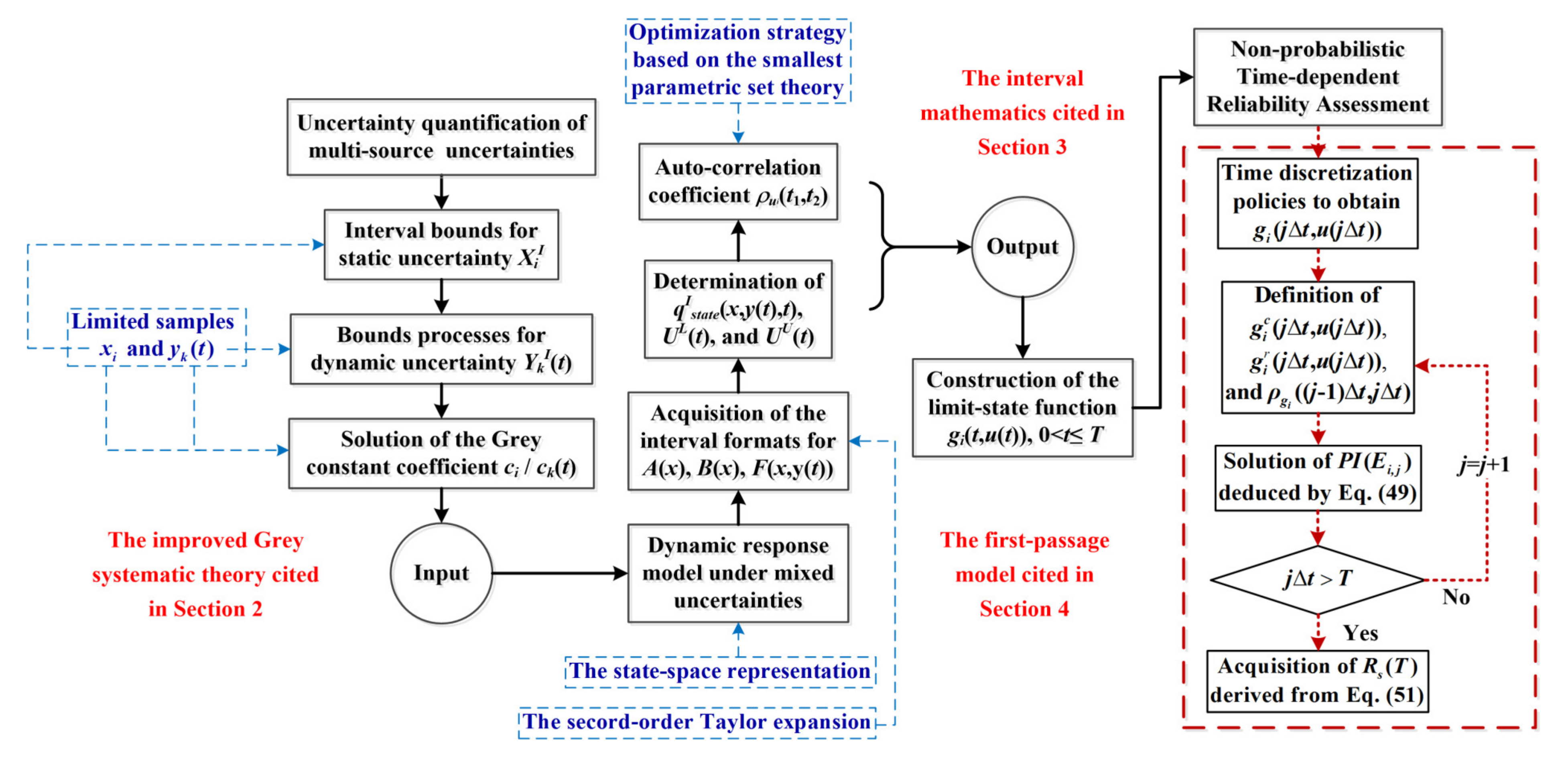
2.2. General Procedure of the Grey System Theory

As stated in Section 2.1, the key to interval UQ analysis is to obtain accurate bounds information from insufficient samples, and thus to conduct the subsequent work of uncertainty propagation and reliability analysis. In this section, the Grey systematic approach in number theory, which regards uncertain static and dynamic parameters as Grey quantities constantly changing in certain scopes, is employed to deal with mechanical uncertainty issues. It does not treat the sample research in the view of finding statistical rules, but also adopts data processing operations to restructure the original rough data to regularly sequence and then gain the bounds information of uncertainties.

Now, take the static case as an example. Suppose a group of measured experimental data corresponding to one specific uncertain variable $x_i$ is listed as

$$X_i=\left\{x_i(l), l=1,2,\dots ,m_1\right\}$$

(10)

where $X_i$ is the sample set of interval variable $x_i$ including $m_1$ data point. Arrange the sequence $X_i$ in turn from small to big, and hence an updated sequence $X_i^{(1)}$ is obtained by

$$X_i^{(1)}=\left\{x_i^{(1)}(1), x_i^{(1)}(2),\dots , x_i^{(1)}(m_1)\right\}$$

(11)

where $x_i^{(1)}(l)\le x_i^{(1)}(l+1), l=1,2,\dots ,m-2$. By accumulating the calculation of the sequence in Equation (11), one can obtain the new form of the data list as

$$\begin{array}{c}{X}_i^{(2)}=\left\{x_i^{(2)}(l), l=1,2,\dots ,m_1\right\}=\left\{x_i^{(2)}(1), x_i^{(2)}(2),\dots , x_i^{(2)}(m_1)\right\}\\ =\left\{x_i^{(1)}(1), x_i^{(1)}(1)+x_i^{(1)}(2),\dots , x_i^{(1)}(1)+x_i^{(1)}(2)+\cdot \cdot \cdot +x_i^{(1)}(m_1)\right\}\end{array}$$

(12)

The definition

$$\left\{\begin{array}{l}{\Delta }_i(l)=\frac{x_i^{(2)}(m_1)}{m_1}\cdot l-x_i^{(1)}(l)\\ {\Delta }_i^{\max }=\max \left({\Delta }_i(l)\right)\\ s_i=c_i\cdot \frac{{\Delta }_i^{\max }}{m_1}\end{array}\right.,l=1,2,\dots ,m_1$$

(13)

$c_i$, named as the Grey constant coefficient, is generally given by empirical cognition based on statistical knowledge and $s_i$ is a quantitative estimation of uncertainty of data $X_i$, which embodies the deviation effect of $x_i$. If the mean value is derived by $\overline{x_i}=\frac{1}{m_1}{\displaystyle \sum _{l=1}^{m_1}{x}_i^{(1)}(l)}$, the UQ result obtained by the Grey model can be eventually taken as

$$x_i\in \left[x_i^L, x_i^U\right]=\left[\overline{x_i}-3s, \overline{x_i}+3s\right]$$

(14)

Obviously, in terms of dynamic uncertainty problems, the available sample curves for $Y_k(t)=\left\{y_k(t,1), y_k(t,2),\dots , y_k(t,n_1)\right\}$ may be degenerated into sample points $Y_k(t_j)=\left\{y_k(t_j,1), y_k(t_j,2),\dots , y_k(t_j,n_1)\right\}$ by time discretization operations, and thus the aforementioned Grey system approach can be directly adopted to obtain the bounds information of the interval process $y_k(t)$.

2.3. Feasible Implementation

Considering that the value of the Grey constant coefficient $c_i$ in Equation (13) is indeed determined by uncertainty samples themselves, a feasible parameter estimation method via limited data set $X_i$ has to be implemented. The motivation procedures are summarized as:

(i) Extraction of data $x_i(1), x_i(2),\dots , x_i(l)$ from original sample set $X_i$, and definitions of the following characteristic quantities by

$${\sigma }_i(l-1)=\sqrt{\frac{1}{l-1}{\left[x_i(l^{*})-\frac{1}{l}{\displaystyle \sum _{l^{*}=1}^l{x}_i(l^{*})}\right]}^2}, l=2,3,\dots ,m_1$$

(15)

and

$$\left\{\begin{array}{l}{\Delta }_i(l^{*})=\frac{x_i^{(2)}(l)}{l}\cdot l^{*}-x_i^{(1)}(l^{*})\\ {\Delta }_i^{\max }(l-1)=\max \left({\Delta }_i(l^{*})\right)\\ d_i(l-1)=\frac{{\Delta }_i^{\max }(l-1)}{l-1}\end{array}\right., l^{*}=1,2,\dots ,l$$

(16)

where ${\sigma }_i(l-1)$ is the sample standard deviation based on the statistical theory.

(ii) Traversal of each value of $l$ from 2 to $m_1$, and establishment of two vectors related to the data sequences by

$${\Sigma }_i={\left[{\sigma }_i(1), {\sigma }_i(2),\dots , {\sigma }_i(m_1-1)\right]}^T \mathrm{and} D_i={\left[d_i(1), d_i(2),\dots , d_i(m_1-1)\right]}^T$$

(17)

(iii) Acquirement of the accumulating sequences of Equation (17) referred by Equations (11) and (12), i.e., ${\Sigma }_i\to {\Sigma }_i^{\left(\mathbf{2}\right)}$ and $D_i\to D_i^{\left(\mathbf{2}\right)}$.

(iv) Construction of the least-square estimation model for fitting the equation shaped like ${\Sigma }_i^{\left(\mathbf{2}\right)}=c_i\cdot D_i^{\left(\mathbf{2}\right)}$, and determination of the optimal estimation $\widehat{c_i}$ by

$$c_i\to \widehat{c_i}={\left({\left(D_i^{\left(\mathbf{2}\right)}\right)}^T\cdot D_i^{\left(\mathbf{2}\right)}\right)}^{-1}\cdot {\left(D_i^{\left(\mathbf{2}\right)}\right)}^T\cdot {\Sigma }_i^{\left(\mathbf{2}\right)}$$

(18)

As discussed earlier, the Grey constant coefficient $c_i$ can be finally confirmed by the insufficient sample data to provide necessary input condition for solving $s_i$, as is shown in Equation (13). Moreover, considering that in some typical cases, the errors in measurement or from an inherent system may be inevitable during the sample extraction process; therefore, the way to eliminate the gross error needs to be explored as well (referred by [36]). To sum up the foregoing comprehensive analysis, the uncertainty bounds for interval variable $x_i$ are available. Similarly, the processes of the lower and upper bounds subjected to the time-varying uncertain parameter $y_k(t)$ can be rationally represented.

3. Dynamic Response Analysis by Utilizing the Interval Quantitative Results

In this section, the time-invariant and time-variant quantitative results obtained by the presented Grey mathematical model will be imposed into the uncertainty propagation analysis for structural dynamics. The interval process model with regard to the structural response can be established based on two aspects of research work: On one hand, the knowledge of the response bound histories is acquired by the Taylor expansion method; on the other hand, the auto-correlation information is ascertained by the optimization technique derived from the minimum envelope idea. In a word, this section actually serves as a connecting link between the preceding UQ analysis and the following time-dependent reliability calculation.

3.1. Uncertainty Estimation with the Series Expansion Approach

Consider the following differential equation of motion about a general dynamical system with $r$ degree as

$$\left\{\begin{array}{l}M\ddot{u}(t)+P\dot{u}(t)+Ku(t)=F(t)\\ u(t_0)=u_0,\dot{u}(t_0)={\dot{u}}_0\end{array}\right.$$

(19)

where $M=(m_{ij})\in {ℝ}^{r\times r}$, $P=(p_{ij})\in {ℝ}^{r\times r}$, $K=(k_{ij})\in {ℝ}^{r\times r}$ are the mass, damping, and stiffness matrices, respectively, $F(t)=\left(f_i(t)\right)\in {ℝ}^{r\times 1}$ means the external load vector, $u(t), \dot{u}(t), \ddot{u}(t)\in {ℝ}^{r\times 1}$ are the response vectors of displacement, velocity and acceleration, and $u(t_0)$ and $\dot{u}(t_0)$ are the corresponding initial conditions.

When the uncertainty influences are taken into consideration, the elements either in constitutive matrixes ($M$, $P$, and $K$) or in external excitation vector $F(t)$ may be valued by the quantitative results of uncertainties $\mathit{x}$ and $y(t)$. In this study, the fluctuation of inherent structural parameters lies on the static uncertainty items, whereas the dispersion of loading conditions is derived from the integration of both static and dynamic issues. Thus, Equation (19) can be rewritten as

$$M(x)\cdot \ddot{u}\left(x,y(t),t\right)+P(x)\cdot \dot{u}\left(x,y(t),t\right)+K(x)\cdot u\left(x,y(t),t\right)=F(x,y(t),t)$$

(20)

In point of fact, the uncertainty propagation problem can be stated as: Input the quantitative models of structural and loading uncertainties as cited in Section 2 (from original samples), and seek a set $\Gamma \in {ℝ}^{r+1}$ of response being consistent with Equation (20), where $\Gamma$ is the feasible domain of the known vector $\mathit{x}$ and $y(t)$, i.e.,

$$\Gamma =\left\{\begin{array}{c}u\left(x,y(t),t\right):M(x)\cdot \ddot{u}\left(x,y(t),t\right)+P(x)\cdot \dot{u}\left(x,y(t),t\right)\\ +K(x)\cdot u\left(x,y(t),t\right)=F(x,y(t),t),\\ x_i\in x_i^I=\left[x_i^L, x_i^U\right],\hspace{0.33em}i=1,2,\cdots ,m \\ y_k(t)\in y_k^I(t)=\left[y_k^L(t), y_k^U(t)\right],\hspace{0.33em}k=1,2,\cdots ,n\end{array}\right\}$$

(21)

The set $\Gamma$ is usually an irregular region, which is difficult to determine accurately. With the concept of interval mathematics, the aim is to find a time-varying hyper-rectangle containing the set $\Gamma$ as closely as possible. According to Equations (1) and (6), it can be noted that the dynamic response $u(t)$ can also be given as a format of interval process, i.e.,

$$u(t)\in u^I\left(x,y(t),t\right)=\left[u^L\left(x,y(t),t\right), u^U\left(x,y(t),t\right)\right]$$

(22)

or the component form

$$u_i(t)\in u_i^I(t)=\left[u_i^L\left(x,y(t),t\right), u_i^u\left(x,y(t),t\right)\right],i=1,2,\dots ,r$$

(23)

For the purpose of obtaining a quick solution for Equations (22) and (23), denote the terms used in structural vibration theory, by describing a state vector with

$$q_{state}(t)={\left[u\left(x,y(t),t\right),\hspace{0.33em}\dot{u}\left(x,y(t),t\right)\right]}^T$$

(24)

Then, the mathematical formulation in Equation (20) can also be expressed in the state-space representation, as defined by

$$\begin{array}{l}{\dot{q}}_{state}(t)=A(x)\cdot q_{state}(t)+B(x)\cdot F\left(x,y(t),t\right)\\ q_{output}(t)=C(x)\cdot q_{state}(t)+D(x)\cdot F\left(x,y(t),t\right)\end{array}$$

(25)

where $q_{output}(t)=\ddot{u}\left(x,y(t),t\right)$ is the output vector, and

$$\begin{array}{l}A(x)=\left[\begin{array}{cc}\mathbf{0}& I\\ -M^{-1}(x)\cdot K(x)& -M^{-1}(x)\cdot P(x)\end{array}\right],B(x)=\left[\begin{array}{c}\mathbf{0}\\ M^{-1}(x)\end{array}\right]\\ C(x)=\left[\begin{array}{cc}-M^{-1}(x)\cdot K(x)& -M^{-1}(x)\cdot P(x)\end{array}\right],D(x)=M^{-1}(x)\end{array}$$

(26)

In order to efficiently and precisely obtain the bounds of the response interval, the second-order Taylor expansion is utilized here, in which the state matrix $A(x)$ and the input matrix $B(x)$ are approximately represented as

$$\begin{array}{cc}\Phi (x)\hfill & =\Phi (x^c+x^r\circ \Psi )\hfill \\ & \approx \Phi (x^c)+{\displaystyle \sum _{i=1}^m\frac{\partial \Phi (x^c)}{\partial x_i}\cdot x_i^r+}\frac{1}{2}{\displaystyle \sum _{i_1,i_2=1}^m\frac{{\partial }^2\Phi (x^c)}{\partial x_{i_1}\partial x_{i_2}}\cdot }{x}_{i_1}^r\cdot x_{i_2}^r=\Phi (x^c)+\delta \Phi \hfill \end{array}$$

(27)

where $\delta$ means an operator for description of the perturbation quantity. Analogously, combined with the time discretization strategy, the external load vector $F(t_j)$ under instant $t_j=j\Delta t$ can be expressed by

$$\begin{array}{c}F\left(x,y(t_j),t_j\right)\approx F\left(x^c,y^c(t_j),t_j\right)\hfill \\ +{\displaystyle \sum _{i=1}^m\frac{\partial F\left(x^c,y^c(t_j),t_j\right)}{\partial x_i}\cdot x_i^r+}{\displaystyle \sum _{k=1}^n\frac{\partial F\left(x^c,y^c(t_j),t_j\right)}{\partial y_k(t_j)}\cdot y_k^r(t_j)}\hfill \\ +\frac{1}{2}{\displaystyle \sum _{i_1,i_2=1}^m\frac{{\partial }^{2}F\left(x^c,y^c(t_j),t_j\right)}{\partial x_{i_1}\partial x_{i_2}}\cdot }{x}_{i_1}^r\cdot x_{i_2}^r+\frac{1}{2}{\displaystyle \sum _{k_1,k_2=1}^n\frac{{\partial }^{2}F\left(x^c,y^c(t_j),t_j\right)}{\partial y_{k_1}(t_j)\partial y_{k_2}(t_j)}\cdot }{y}_{k_1}^r(t_j)\cdot y_{k_2}^r(t_j)\hfill \\ =F\left(x^c,y^c(t_j),t_j\right)+\delta F(t_j)\hfill \end{array}$$

(28)

.

Obviously, it can also be defined as

$$q_{state}(t_j)\approx q_{state}\left(x^c,y^c(t_j),t_j\right)+\delta q_{state}(t_j)$$

(29)

When substituting Equations (27)–(29) together with Equation (25), we have

$$\begin{array}{cc}{\dot{q}}_{state}\left(x^c,y^c(t_{j+1}),t_{j+1}\right)+\delta {\dot{q}}_{state}(t_{j+1})\hfill & =\left[A(x^c)+\delta A\right]\cdot \left[q_{state}\left(x^c,y^c(t_j),t_j\right)+\delta q_{state}(t_j)\right]\hfill \\ & +\left[B(x^c)+\delta B\right]\cdot \left[F\left(x^c,y^c(t_j),t_j\right)+\delta F(t_j)\right]\hfill \end{array}$$

(30)

Then, the following expressions can be obtained by ignoring the high order items, namely,

$${\dot{q}}_{state}\left(x^c,y^c(t_{j+1}),t_{j+1}\right)=A(x^c)\cdot q_{state}\left(x^c,y^c(t_j),t_j\right)+B(x^c)\cdot F\left(x^c,y^c(t_j),t_j\right)$$

(31)

and

$$\begin{array}{cc}\delta {\dot{q}}_{state}(t_{j+1})\hfill & =A(x^c)\cdot \delta q_{state}(t_j)+\delta A\cdot q_{state}\left(x^c,y^c(t_j),t_j\right)\hfill \\ & +B(x^c)\cdot \delta F(t_j)+\delta B\cdot F\left(x^c,y^c(t_j),t_j\right)\hfill \end{array}$$

(32)

With the precise time integration method, $q_{state}\left(x^c,y^c(t),t\right)$ and $\delta q_{state}(t)$ can be explicitly reconstructed. According to the natural interval extension, in Equation (29) we obtain

$$q_{state}^I\left(x,y(t),t\right)=q_{state}\left(x^c,y^c(t),t\right)+\mathsf{\Delta }{q}_{state}^I(t)$$

(33)

where $\mathsf{\Delta }{q}_{state}^I(t)=\left[-\left|\delta q_{state}(t)\right|, \left|\delta q_{state}(t)\right|\right]$. Ultimately, the lower and the upper bounds of the response intervals may be arrived at by

$$u^L\left(x,y(t),t\right)=u\left(x^c,y^c(t),t\right)-\left|\delta u(t)\right| \mathrm{and} u^U\left(x,y(t),t\right)=u\left(x^c,y^c(t),t\right)+\left|\delta u(t)\right|$$

(34)

where the value of the perturbation item $\delta u(t)$ lies on the iterative calculations deduced by the foregoing Equations (24)–(33).

3.2. Correlation Representation Achieved by Novel Optimization-Based Strategy

As per the statements discussed in Section 3.1, the uncertainty bounds of the dynamic responses $u_i(t), i=1,2,\dots ,r$ can be obtained, and indeed it can be regarded as interval processes. However, based on the definitions of the time-variant interval model cited in Section 2.1, the characteristics of the auto-correlation between $u_i(t_1)$ and $u_i(t_2)$ should be confirmed as well. In view of this, this study employs a novel optimization method based on the conception of the smallest parametric interval set to deal with this correlation issue.

(a) Firstly, the common method for determining the smallest ‘box’ (i.e., one hyper-rectangle in essence) containing multi-dimensional sample data is investigated. Considering the case that the uncertain parameters ${\alpha }_i$ ($i=1,2,\dots ,s$) constitute an $s$-dimensional parametric space with limited information containing $S$ sample points, namely, ${\alpha }_i^{(S)}=\left\{a_i(1), {\alpha }_i(2),\dots , {\alpha }_i(S)\right\}$, the expression of the transformation matrix thus reads as

$$T(\theta )=({\delta }_1, {\delta }_2,\cdots , {\delta }_s)$$

(35)

where $\theta =({\theta }_i) (i=1,2,\dots ,s-1)$ is the vector of rotation angles relative to the original coordinate, and

$${\delta }_j=\left\{\begin{array}{c}{0}_{j-2}\\ {\tilde{\delta }}_j\end{array}\right\}$$

(36)

where $0_{j-2}$ means a column vector with $j-2$ zero items, and ${\tilde{\delta }}_j$ is deduced by

$${\tilde{\delta }}_j=\left(\begin{array}{c}-\mathit{sin}{\theta }_{j-1}\\ \mathit{cos}{\theta }_{j-1}\mathit{cos}{\theta }_j\\ ⋮\\ \mathit{cos}{\theta }_{j-1}\mathit{sin}{\theta }_j\cdots \mathit{sin}{\theta }_{s-2}\mathit{cos}{\theta }_{s-1}\\ \mathit{cos}{\theta }_{j-1}\mathit{sin}{\theta }_j\cdots \mathit{sin}{\theta }_{s-2}\mathit{sin}{\theta }_{s-1}\end{array}\right)$$

(37)

Each element of the original sample set ${\alpha }_i^{(S)}$ will be transferred to ${\beta }_i^{(S)}$ with the transformation matrix $T(\theta )$ (from $\alpha$-space to $\beta$-space). With the aim of determining the smallest interval set to envelope all the samples, the $s$-dimensional ‘box’ should be examined by

$$\left|\beta -{\beta }^c\right|\le {\beta }^r$$

(38)

where the center vector ${\beta }^c={({\beta }_1^c, {\beta }_2^c,\cdots , {\beta }_s^c)}^T$ and the semi-axis vector ${\beta }^r={({\beta }_1^r, {\beta }_2^r,\cdots , {\beta }_s^r)}^T$. The components ${\beta }_i^c$ and ${\beta }_i^r$ are given by

$${\beta }_i^c=\frac{1}{2}\left(\underset{S}{\max }\left({\beta }_i^{(S)}\right)+\underset{S}{\min }\left({\beta }_i^{(S)}\right)\right) \mathrm{and} {\beta }_i^r=\frac{1}{2}\left(\underset{S}{\max }\left({\beta }_i^{(S)}\right)-\underset{S}{\min }\left({\beta }_i^{(S)}\right)\right)$$

(39)

Then, the hyper-volume of the ‘box’ in Equation (38) is calculated by

$$V_{hyper}={\displaystyle \prod _{i=1}^s{(2{\beta }_i^r)}^s}$$

(40)

which is a function of the rotation angles ${\theta }_i$. The best interval set or the hyper-rectangle among all possible boxes should be the one that envelopes all the given sample points with the minimum volume, namely,

$$V_{hyper}^{*}=\underset{{\theta }^{*}}{\min }{V}_{hyper}({\theta }_1,{\theta }_2,\dots ,{\theta }_{s-1})$$

(41)

To rapidly solve the optimization formulas as shown in Equation (41), either the gradient algorithm based on sensitivity information or the intelligent algorithm using population evolution has to be attached. After the minimum $V_{hyper}^{*}$ is obtained by optimization, the optimal design parameters ${\theta }_i^{*}$ can reflect the correlation between the uncertain parameters ${\alpha }_i$ and ${\alpha }_{i+1}$.

(b) In fact, for the interval process $u_i(t)$, the correlation properties between $u_i(t_1)$ and $u_i(t_2)$ with any instant times $t_1$ and $t_2$ make sense. The above optimization procedure can be carried out by following steps:

(i) By utilizing the orthogonal test design under available static and dynamic uncertainty data, take all the sample combinations into deterministic differential equation as shown in Equation (19), and then acquire the set of response curves $u_i^{(S)}(t)=\left\{u_i(t,1), u_i(t,2),\dots , u_i(t,S)\right\}$.

(ii) Assume a sufficiently small increment $\Delta t$, and conduct the time-discretization operation to obtain

$$u_i^{(S)}(t_1)=\left\{u_i(t_1,1), u_i(t_1,2),\dots , u_i(t_1,S)\right\}$$

(42)

and

$$u_i^{(S)}(t_2)=\left\{u_i(t_2,1), u_i(t_2,2),\dots , u_i(t_2,S)\right\}$$

(43)

where $t_1=j_1\Delta t$ and $t_2=j_2\Delta t$ ($j_1,j_2=1,2,\dots$).

(iii) Construct a two-dimensional rectangle space ($u_i(t_1)$ − $u_i(t_2)$) generated from Equations (42) and (43), and obtain the smallest rotary rectangular domain (as shown in Figure 1) according to Equation (41), with rotation angel ${\theta }_i^{*}(t_1,t_2)$ and the two semi-axes ${\beta }_i^r(t_1)$ and ${\beta }_i^r(t_2)$.

(iv) According to the smallest interval set, the auto-covariance function $Co{v}_{u_i}(t_1,t_2)$ can be given by

$$Co{v}_{u_i}(t_1,t_2)=\frac{{\left({\beta }_i^r(t_1)\right)}^2-{\left({\beta }_i^r(t_2)\right)}^2}{3}\cdot \sin {\theta }_i^{*}(t_1,t_2)\cdot \cos {\theta }_i^{*}(t_1,t_2)$$

(44)

Similarly, referred by Equation (9), the auto-correlation coefficient function ${\rho }_{u_i}(t_1,t_2)$ reads

$${\rho }_{u_i}(t_1,t_2)=\frac{Co{v}_{u_i}(t_1,t_2)}{\left|\delta u_i(t_1)\right|\cdot \left|\delta u_i(t_2)\right|}$$

(45)

(v) By traversing all the response components $u_i(t)$, the auto-correlation characteristics of the interval process vector $u(t)$ are eventually gained.

In summary, this section presents an integral process of uncertainty propagation analysis via limited time-invariant and time-variant sample data. It is noted that the reliability estimation will be expounded on the basis of the dynamic response results. Therefore, the more precisely we can obtain the bounds properties as well as the auto-correlation descriptions of $u_i(t)$, the more reliable safety evaluation will be achieved. In fact, the work in Section 2 and Section 3 provides the necessary data entry condition for the following structural time-dependent reliability analysis under circumstances of missing information.

4. Non-Probabilistic Time-Dependent Reliability Assessment

For the structural safety, the comparison between the actual performance $u_i(t)$ and the criteria value $u_i^{cr}(t)$ over the analyzed time $[0,T]$ are usually of more concern. Nevertheless, once the uncertainty factors originating from insufficient samples are taken into account, traditional deterministic analysis or the time-invariant probabilistic reliability theory may not be feasible. In view of this, we further define the non-probabilistic time-dependent reliability index as

$$R_s(T)=1-P_f(T)=Pos\left\{\forall t\in \left[0,T\right]:\underset{i\le r}{min}\left[g_i\left(t,u(t)\right)=u_i^{cr}(t)-u_i(t)\right]>0\right\}$$

(46)

where $R_s(T)$ and $P_f(T)$ are the measurements of safety and failure, respectively, $Pos\left\{\cdot \right\}$ means the possibility of a specific event, $\underset{i\le r}{min}\left[\cdot \right]$ represents the minimum, and $g_i\left(t,u(t)\right)$ stands for the time-varying limit state.

It is extremely hard to obtain the analytical solution of Equation (46) in general. To solve this problem, some approximation methods should be used. Based on the classical first-passage theory in random process, Equation (46) can be translated by

$$R_s(T)=1-P_f(T)=1-\underset{i\le r}{\mathit{max}}\left[Pos\left\{\left(g_i\left(0,u(0)\right)<0\right)\cup \left(N_i^{+}(0,T)>0\right)\right\}\right]$$

(47)

where $\underset{i\le r}{\mathit{max}}\left[\cdot \right]$ represents the maximum, $g_i\left(0,u(0)\right)$ means the initial state, and $N_i^{+}(0,T)>0$ denotes the number of upcrossings of zero-value by the processes $g_i\left(t,u(t)\right)$ from the safe domain to the failure domain during $[0,T]$.

The basic simplification in the first-passage theory is that the crossing from the non-failure into the failure domain at each moment is regarded as independent from others. Under such circumstances, $R_s(T)$ arrives at

$$R_s(T)=1-P_f(T)=1-\underset{i\le r}{\mathit{max}}\left[Po{s}_i(0)-{\displaystyle \sum _{j=1}^{N}PI(E_{i,j})}\right],N=\frac{T}{\Delta t}$$

(48)

where $Po{s}_i(0)$ means the possibility of failure at the initial moment $t=0$ and $PI(E_{i,j})$ is the possibility index of the event $E_{i,j}$, which can be expressed as $g_i\left((j-1)\Delta t,u\left((j-1)\Delta t\right)\right)>0\cap g_i\left(j\Delta t,u(j\Delta t)\right)\le 0$.

It is obvious that the possibility index $PI(E_{i,j})$ in Equation (48) depends on the interference of the limit-state functions ($g_i\left((j-1)\Delta t\right)>0$ and $g_i(j\Delta t)\le 0$) and the feasible rectangular domain generated from $g_i\left((j-1)\Delta t\right)$ and $g_i(j\Delta t)$. The possibility index of $E_{i,j}$ is defined as the ratio of the interference area to the feasible rectangular area after normalization, i.e.,

$$PI(E_{i,j})=Pos\left\{g_i\left((j-1)\Delta t,u\left((j-1)\Delta t\right)\right)>0\cap g_i\left(j\Delta t,u(j\Delta t)\right)\le 0\right\}={\left.\frac{A_{\mathit{interference}}}{A_{total}}\right|}_{i,j}$$

(49)

Figure 2 embodies the novel solution method, in which

$$g_i^c\left(t,u(t)\right)=u_i^{cr}(t)-u_i^c(t),g_i^r\left(t,u(t)\right)=u_i^r(t),{\rho }_{g_i}\left((j-1)\Delta t,j\Delta t\right)={\rho }_{u_i}\left((j-1)\Delta t,j\Delta t\right)$$

(50)

Substitution of Equation (49) into Equation (48) yields

$$R_s(T)=1-\underset{i\le r}{\mathit{max}}\left[Po{s}_i(0)-{\displaystyle \sum _{j=1}^N{\left.\frac{A_{\mathit{interference}}}{A_{total}}\right|}_{i,j}}\right]$$

(51)

As mentioned above, to form the limited samples, the entire theoretical contents from quantization and propagation of static and dynamic uncertainties to structural safety estimation based on non-probabilistic time-dependent reliability have been expounded (as shown in Figure 3). In the next two sections, the effectiveness of the proposed method will be proven by numerical and experimental examples.

5. Numerical Example

In this section, the provided approach is used to solve a practical engineering problem (the safety prediction of the laminated composite plates) under limited static and dynamic uncertainty information. Firstly, uncertainty quantification (UQ) analysis via actual experimental samples (insufficient static samples of material properties $E_1$, $E_2$, ${\nu }_{12}$, and $G_{12}$), as well as virtual simulation data (few time-variant history curves for description of the uncertain dynamic load $F(t)$), is conducted to determine the boundary rules of input parameters. The uncertainty propagation analysis for acquisition of the lower and upper bounds of allowable load ($F_{allow}^L(t)$ and $F_{allow}^U(t)$) is then carried out by virtue of the quantified results. As per the uncertainty features of $F(t)$ (the bounds and the correlation characteristics) and the calculated response result $F_{allow}(t)$, the time-dependent reliability estimation is eventually accomplished, and the comparisons based on the Monte Carlo method are involved to prove the validity and effectiveness of the investigated study. For details, see the subsequent statements.

5.1. Cases of Time-Invariant and Time Variant Uncertainty Quantification Analysis

As the necessary input conditions for the subsequent reliability assessment of the composite laminates, the achievement of the quantitative study with limited sample data is of great importance. Here, a total of two cases, namely, the static one under 16 groups of actual experimental samples corresponding to the engineering constants $E_1$, $E_2$, ${\nu }_{12}$, and $G_{12}$ of T300/QY8911 (as listed in

Table 1. Experimental data of the engineering constants for T300/QY8911.

No.	$$\begin{gathered} {\mathit{E}}_1 \\ \left(\mathbf{GPa}\right) \end{gathered}$$	$$\begin{gathered} {\mathit{E}}_2 \\ \left(\mathbf{GPa}\right) \end{gathered}$$	${\mathit{v}}_{12}$	$$\begin{gathered} {\mathit{G}}_{12} \\ \left(\mathbf{GPa}\right) \end{gathered}$$	$$\begin{gathered} {\mathit{E}}_1 \\ \left(\mathbf{GPa}\right) \end{gathered}$$	No.	$$\begin{gathered} {\mathit{E}}_1 \\ \left(\mathbf{GPa}\right) \end{gathered}$$	$$\begin{gathered} {\mathit{E}}_2 \\ \left(\mathbf{GPa}\right) \end{gathered}$$	${\mathit{v}}_{12}$	$$\begin{gathered} {\mathit{G}}_{12} \\ \left(\mathbf{GPa}\right) \end{gathered}$$
1	129.20	9.34		0.28	5.23	9	132.19	9.07	0.30	4.85
2	131.59	9.53		0.33	4.97	10	132.00	9.73	0.35	5.00
3	130.63	9.08		0.33	5.16	11	130.39	9.21	0.34	5.34
4	132.01	9.34		0.33	5.15	12	128.28	8.67	0.33	4.98
5	131.04	8.94		0.34	5.15	13	135.30	9.18	0.32	5.13
6	120.61	9.04		0.33	4.81	14	137.33	9.28	0.33	5.25
7	127.69	8.99		0.32	5.11	15	141.69	10.73	0.31	5.47
8	133.65	9.36		0.35	5.08	16	126.91	9.39	0.33	5.45

, which is referred by [26]) and the dynamic one under six groups of virtual simulation histories subjected to external excitation $F(t)$ (as shown in Figure 4, which is modified by [37,38]) are analyzed by utilizing the improved Grey system theory as above discussed. For ease of understanding, we take the longitudinal elastic modulus $E_1$ as an example, and its specific quantification procedure is summarized below.

In accordance with Equations (10) and (11), the experimental data points of $E_1$ can be listed as

$$\begin{array}{ccc}{E}_1^{(1)}& =& \left\{E_1^{(1)}(1), E_1^{(1)}(2),\dots , E_1^{(1)}(16)\right\}\hfill \\ & =& \left\{120.61, 126.91, 127.69, 128.28, 129.20, 130.39, 130.63, 131.04,\right.\hfill \\ & & \left.131.59, 132.00, 132.01, 132.19, 133.65, 135.30, 137.33, 141.69\right\}\hfill \end{array}$$

(52)

After the accumulation, the above sequence will be expressed as $E_1^{(2)}$, i.e.,

$$\begin{array}{lll}{E}_1^{(2)}& =& \left\{120.61, 247.52, 375.21, 503.49, 632.69, 763.08, 893.71, 1024.75,\right.\hfill \\ & & \left.1156.34, 1288.34, 1420.35, 1552.54, 1686.19, 1821.49, 1958.82, 2100.51\right\}\hfill \end{array}$$

(53)

Substituting Equation (53) into Equation (13) yields

$${\Delta }_{E_1}^{\max }=\max \left({\Delta }_{E_1}(l)\right)=\max \left(\frac{E_1^{(2)}(16)}{16}\cdot l-E_1^{(1)}(l)\right)=25.505$$

(54)

In terms of Equations (15)–(17) cited in Section 2.3, we further obtain

$$\begin{array}{ccc}{\Sigma }_{E_1}& =& {\left[{\sigma }_{E_1}(1), {\sigma }_{E_1}(2),\dots , {\sigma }_{E_1}(15)\right]}^T\hfill \\ & =& \left[4.4548, 3.8821, 3.5529, 3.4179, 3.4378, 3.3984, 3.3640,\right.\hfill \\ & & {\left.3.3556, 3.3536, 3.3225, 3.2893, 3.3647, 3.5616, 3.9061, 4.6844\right]}^T\hfill \end{array}$$

(55)

and

$$\begin{array}{ccc}{D}_{E_1}& =& {\left[d_{E_1}(1), d_{E_1}(2),\dots , d_{E_1}(15)\right]}^T\hfill \\ & =& \left[1.5750, 1.4867, 1.3156, 1.1856, 1.1400, 1.1180, 1.1339,\right.\hfill \\ & & {\left.1.1599, 1.1846, 1.1819, 1.1835, 1.2188, 1.2744, 1.3632, 1.5941\right]}^T\hfill \end{array}$$

(56)

After a second accumulation and substitution of Equations (55) and (56) together with (18), the optimal estimation $\widehat{c_{E_1}}$ reads as

$$c_{E_1}\to \widehat{c_{E_1}}={\left({\left(D_{E_1}^{\left(\mathbf{2}\right)}\right)}^T\cdot D_{E_1}^{\left(\mathbf{2}\right)}\right)}^{-1}\cdot {\left(D_{E_1}^{\left(\mathbf{2}\right)}\right)}^T\cdot {\Sigma }_{E_1}^{\left(\mathbf{2}\right)}=2.8361$$

(57)

Thus, the quantitative interval can be given as

$$E_1\in \left[E_1^L, E_1^U\right]=\left[\overline{E_1}-3\cdot \widehat{c_{E_1}}\cdot \frac{{\Delta }_{E_1}^{\max }}{16}, \overline{E_1}+3\cdot \widehat{c_{E_1}}\cdot \frac{{\Delta }_{E_1}^{\max }}{16}\right]=\left[117.7189, 144.8448\right] GPa$$

(58)

The detailed process for quantifying the uncertainty of $E_1$ is exhibited by the presented approach. Moreover, all bounds results with reference to other static uncertain variables ($E_2$, ${\nu }_{12}$, and $G_{12}$), as well as the dynamic load history $F(t)$, can be also obtained via the limited samples, as shown in

Table 2. Quantification results for static uncertainty characteristics $E_1$ $E_2$, ${\nu }_{12}$, and $G_{12}$.

	The Grey Constant Coefficient	The Mean Value	The Lower Bound	The Upper Bound
$E_1$	$c_{E_1}=2.8361$	$E_1^c=131.2819$	$E_1^L=117.7189$	$E_1^U=144.8448$
$E_2$	$c_{E_2}=2.7582$	$E_2^c=9.3050$	$E_2^L=8.1233$	$E_2^U=10.4867$
$v_{12}$	$c_{{\nu }_{12}}=2.6793$	${\nu }_{12}^c=0.3263$	${\nu }_{12}^L=0.2754$	${\nu }_{12}^U=0.3771$
$G_{12}$	$c_{G_{12}}=2.5181$	$G_{12}^c=5.1456$	$G_{12}^L=4.5625$	$G_{12}^U=5.7287$

and Figure 5; Figure 5 also manifests the change trend of the Grey constant coefficient $c_F(t)$. Apparently, the quantified results will be applied into the following composite structures for response calculation and time-dependent reliability estimation.

5.2. Cases of Time-Dependent Reliability Evaluation via Available Quantified Results

Here, a 12-layer composite laminates plate ${\left[\theta /\theta /\theta -\theta /-\theta /-\theta \right]}_{sym}$ under one concentrated load in the geometric center with four clamped supported sides is studied. The length $l$ and width $b$ of the plate are $l=b=120\mathrm{mm}$, with a thickness of $t=0.3\mathrm{mm}$ for each lamina. The material of the lamina is transversely isotropic with a density of $\rho =1.38\times {10}^3\mathrm{kg}/{\mathrm{m}}^3$.

Table 3. Basic strength variables of the laminated composite plate (unit: $GPa$).

${\mathit{X}}_{\mathit{t}}$	${\mathit{X}}_{\mathit{c}}$	${\mathit{Y}}_{\mathit{t}}$	${\mathit{Y}}_{\mathit{c}}$	$\mathit{S}$
$1.5372\times \alpha (t)$	$1.7221\times \alpha (t)$	$0.0444\times \alpha (t)$	$0.2139\times \alpha (t)$	$0.1024\times \alpha (t)$

in which $\alpha (t)=\exp (-0.005t)$ ($t\in \left[0, T\right], T=20 \mathrm{years}$).

shows the basic strength variables of this composite plate, in which the strength degeneration index is defined as $\alpha (t)$ ($t\in \left[0, T\right], T=20 \mathrm{years}$).

In common deterministic analysis, the key point of the first-layer failure judgment relies on solving the allowable load $F_{allow}$, which can be confirmed by finite element analysis. In this problem, each lamina is divided into 2500 elements. Therefore, there are 30,000 elements for the whole plate (as shown in Figure 6), which may guarantee a high accuracy result. According to the Tsai–Wu strength criterion, $F_{allow}$ can be obtained from

$$\begin{array}{l}{F}_{allow}=\min (F^i,T)\\ s.t. F_1(T)\cdot {\sigma }_1(F^i,T)+F_2(T)\cdot {\sigma }_2(F^i,T)+F_{11}(T)\cdot {\sigma }_1^2(F^i,T)+F_{22}(T)\cdot {\sigma }_2^2(F^i,T)\\ +F_{66}(T)\cdot {\tau }_{12}^2(F^i,T)+2F_{12}(T)\cdot {\sigma }_1(F^i,T)\cdot {\sigma }_2(F^i,T)=1\end{array}$$

(59)

where $F_1(T)=\alpha (T)\cdot \left(\frac{1}{X_t}-\frac{1}{X_c}\right)$, $F_2(T)=\alpha (T)\cdot \left(\frac{1}{Y_t}-\frac{1}{Y_c}\right)$, $F_{11}(T)=\frac{\alpha (T)}{X_t\cdot X_c}$, $F_{22}(T)=\frac{\alpha (T)}{Y_t\cdot Y_c}$, $F_{66}(T)=\frac{\alpha (T)}{S^2}$, $F_{12}(T)=-\frac{\alpha (T)}{2\sqrt{X_t\cdot X_c\cdot Y_t\cdot Y_c}}$, $F^i$ means the failure load of the $i$th lamina, ${\sigma }_1(F^i,T)$, ${\sigma }_2(F^i,T)$, and ${\tau }_{12}(F^i,T)$ are the longitudinal normal stress, the transverse normal stress, and the shear stress under $F^i$ and $T$, respectively.

Nevertheless, once the uncertainties, which exist in material properties, are considered (from the quantitative results in Table 2), it will be more complicated to solve Equation (59), and the allowable load $F_{allow}$ will be converted into an interval process, rather than a specific value any more. In such circumstances, the proposed uncertainty propagation method cited in Section 3.1 can be directly adopted by a combination of the finite difference conceptions and the interval mathematics, and the fast boundary solutions with changing ply angle $\theta$ are given. Figure 7 summarizes some results of $F_{allow}^L(t)$ and $F_{allow}^U(t)$ under typical cases of $\theta$. Thus, associated with the previous quantified interval process $F(t)$, the safety measurement of this composite laminate becomes

$$R_s(T)=Pos\left\{\forall t\in \left[0,T\right]:g\left(F_{allow}(t), F(t)\right)=F_{allow}(t)-F(t)>0\right\}$$

(60)

where the time independency effect of the limit state $g\left(F_{allow}(t), F(t)\right)$ lies in the co-relationship of the interval process $F(t)$, in essence. With the help of the novel optimization-based strategy in this study, the auto-correlation coefficient function ${\rho }_F\left((j-1)\Delta t,j\Delta t\right)$ can be determined by the sample curves in Figure 4. Figure 8 shows the details. Therefore, associated with the above uncertainty quantification and propagation results, the presented non-probabilistic time-dependent reliability assessment can be eventually executed, as shown in

Table 4. Non-probabilistic time-dependent reliability results versus different values of ply angel $\theta$.

	${\mathit{R}}_{\mathit{s}}(\mathit{t})$	${\mathit{R}}_{\mathit{s}}(\mathit{t}\le 14)$	${\mathit{R}}_{\mathit{s}}(\mathit{t}=15)$	${\mathit{R}}_{\mathit{s}}(\mathit{t}=16)$	${\mathit{R}}_{\mathit{s}}(\mathit{t}=17)$	${\mathit{R}}_{\mathit{s}}(\mathit{t}=18)$	${\mathit{R}}_{\mathit{s}}(\mathit{t}=19)$	${\mathit{R}}_{\mathit{s}}(\mathit{T})$
$\mathit{\theta }$
$\theta ={15}^{\circ }$		1	0.9997	0.9704	0.9223	0.8998	0.8394	0.8185
$\theta ={30}^{\circ }$		1	1	1	0.9993	0.9913	0.9871	0.9771
$\theta ={45}^{\circ }$		1	1	1	0.9910	0.9757	0.9526	0.9338
$\theta ={60}^{\circ }$		1	0.9918	0.9855	0.9528	0.9398	0.9039	0.8370

and Figure 9. For comparison purposes, the classical probability method based on the Monte Carlo simulations (1,000,000 samples) is also employed to verify the feasibility and rationality of our work, as is demonstrated in Figure 10.

5.3. Discussions on the Results

Synthesizing the computational results of the laminate composite example, the following points can be inherited:

(1)

From the aspect of uncertainty quantification, the quantitative results derived from the Grey systematic theory (with respect to either the static variables $E_1$, $E_2$, ${\nu }_{12}$, $G_{12}$, or the dynamic process $f(t)$) may better envelop the initial data, as is embodied in Table 2 and Figure 5. Moreover, as an improvement for the traditional Grey model, the way of determination of the Grey constant coefficients is a more precise treatment for UQ analysis under small sample limitations. Indeed, it will, to a certain degree, avoid undesirable interval extension effects by using the relationship of the topological locations among all the sample points/curves.

(2)

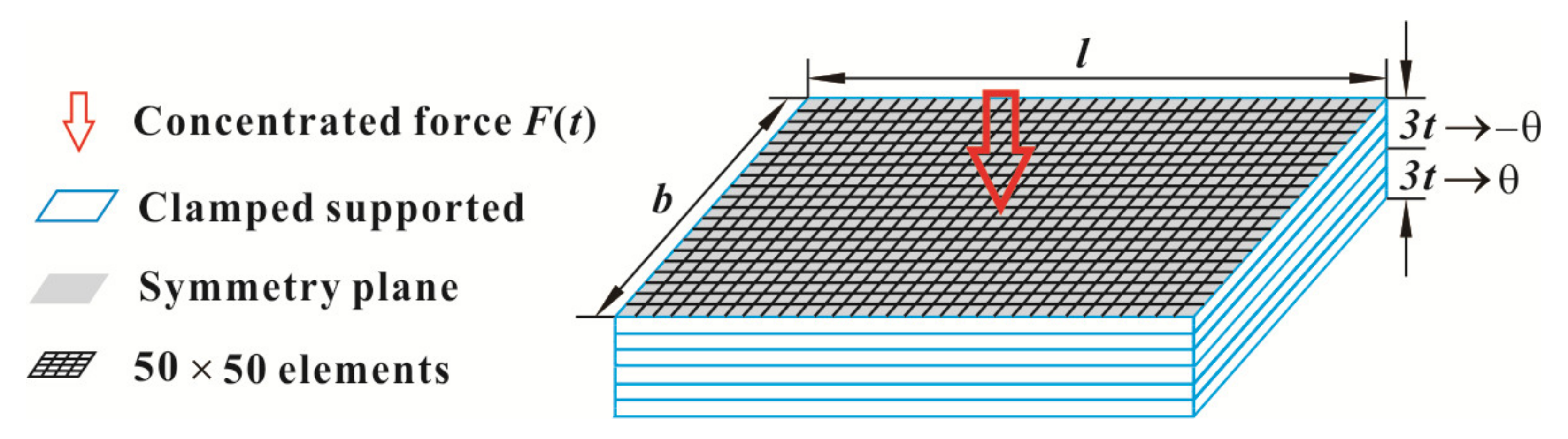
From the point of uncertainty propagation, the developed methodology combined with the state-space transformation and the second-order Taylor expansion may effectively calculate $F_{allow}^L(t)$ and $F_{allow}^U(t)$, although the factors of material dispersion (as summarized in (1)), the material degeneration $\alpha (t)$, and the changing ply patterns ($\theta ={15}^{\circ }, {30}^{\circ },{ 45}^{\circ },{ 60}^{\circ }$) are all taken into account. Furthermore, it should also be indicated that, compared with metal structures, the uncertainty influences in composite structures are much more obvious, and the mechanical performances under different ply angels $\theta$ vary even more (if $\theta ={45}^{\circ }\to F_{allow}^L(T)=1651.85 N$, but if $\theta ={60}^{\circ }\to F_{allow}^L(T)=1161.12 N$).

(3)

From the prospect of safety estimation, the time-dependent reliability obtained by the present analytical method matches the one derived from the Monte Carlo method, as we expected (the accuracy verification). However, there are two aspects that should be stressed: For one thing, the results on the basis of former non-probabilistic method are a little more conservative because of fewer assumptions made about the quantified uncertainties (based on the engineering practice). Furthermore, the accuracy of the reliability results from the Monte Carlo method greatly depends on the amount of samples (1,000,000 samples in the example), which means a computation-intensive and time-consuming situation has to be faced (the superiority of efficiency).

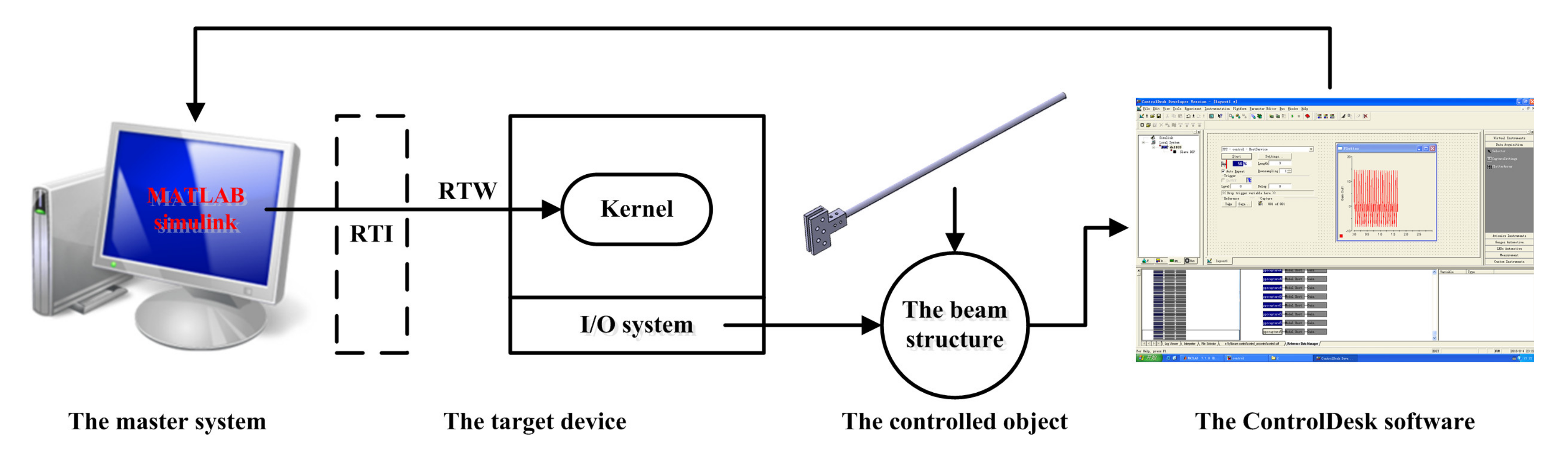
6. Test Verification

In order to verify the practicability of the proposed method in practical engineering, one more experiment for a specific cantilever beam under active vibration control is provided. As is shown in Figure 11, a constant-amplitude sine load is applied to the free end of the cantilever beam. For available reduction of the displacement response (the absolute value of the displacement response should be no more than $u^{cr}=12.5 \mathrm{mm}$), active control force is required. The details of the beam are: the elastic modules $E=70 \mathrm{GPa}$, Poisson’s ratio $\nu =0.3$, and cross-section area $A=100\pi {\mathrm{mm}}^2$. Additionally, five cases of the geometric length $L=400 \mathrm{mm}\to 404 \mathrm{mm}$ are investigated.

In this experiment, the close-loop response of the cantilever beam structure is obtained by the semi-physical simulation platform dsPACE, which contains a master computer, a prototype, a Input/Output (I/O) system, a DS1103 controller board, and test software ControlDesk, as shown in Figure 12 to monitor the close-loop response of the controlled beam.

Considering that there will be many unknown factors, e.g., noise, assembly errors, signal delays, etc. which can influence the results of the close-loop response during the whole experiment, the reliability estimation of the controlled performances is particularly necessary. Therefore, the following process is performed: (1) 35 sets of real experiment samples of close-loop responses ${\left.u(t)\right|}_L$ are measured and recorded. (2) Five initial sets of response data are chosen to conduct the presented UQ and calculate the correlation properties ${\rho }_{u|L}\left((j-1)\Delta t,j\Delta t\right)$. (3) Associated with the critical response value, the time-varying limit-state function $g(t)={\left.u(t)\right|}_L-u^{cr}$ is obtained, and the non-probabilistic time-dependent reliabilities of five different cases are respectively calculated ($T=4 s$). (4) With the aim of calibration, the other 30 sets of samples are used to generate more virtual data (additional 1,000,000 samples in this test), and statistical reliability results are obtained and compared with the ones obtained by the provided method.

In accordance with the above procedures, the uncertainty analysis and time-dependent reliability evaluation of the cantilever beam are well launched under limited experimental sample curves. Figure 13 and Figure 14 show the detailed solution and comparison results. The conclusions in accuracy and effectiveness are similar to the aforementioned numerical examples. Moreover, the reliability calculated by the two methods decreases with the increase of the beam length $L$. Indeed, the increasing $L$ may enlarge the sensitivity level of close-loop responses with respect to uncertainties, and has an adverse impact on reliability.

7. Conclusions

As is known to all, uncertainties widely exist in practical engineering, so that more and more attention has been paid to uncertain structural analysis and design in recent decades. Nevertheless, most of the current studies mainly focus on uncertainty issues (the uncertain response prediction and the structural reliability evaluation) with predetermined parametric descriptions, such as the assumed probability density functions or the given interval bounds for characterizing the uncertain parameters, instead of regarding the uncertainty sample data as the starting point to conduct the subsequent research. Additionally, due to the complexity of multi-source uncertainties in mechanics, which commonly contain time-invariant and time-variant uncertain factors simultaneously, traditional methods of static response analysis and probabilistic reliability assessment may not be feasible anymore with insufficient uncertainty information of discrete sample points/curves.

In view of the aforementioned statements, this study presents an integral analytical procedure containing the UQ, the uncertainty propagation, and the time-dependent reliability estimation under small-scale static and dynamic measurements. The improved Grey mathematical theory is firstly introduced to confirm the boundary laws of uncertainties with the help of the time-invariant and time-variant data, and the topology relations among all the sample locations determine the value of the Grey constant coefficient. Through the quantified bounds results, the dynamic responses can be modeled by interval processes and then calculated by a combination of techniques, such as the second-order Taylor expansion (calculation of the response bounds), as well as the smallest parametric interval set (characteristics of the time dependency). Enlightened by the first-passage theory in random process, the non-probabilistic time-dependent reliability is further defined and analytically solved for realization of the risk estimation of real time-varying structural systems. The rationality and effectiveness of the investigated approach are eventually verified by numerical examples and experimental applications.

Certainly, the purpose of this paper is not to replace other uncertain analysis methods in response computation and reliability measurement. We only wish to propose a possible alternative way when inadequate data is available. It can be concluded that the methods of the uncertainty analysis depends on the type and amount of available data.

References

1. Choi, J.-H.; Jensen, J.J.; Nielsen, U.D. Estimation of Extreme Roll Motion Using the First Order Reliability Method. In Practical Design of Ships and Other Floating Structures; Springer: Singapore, 2019; pp. 682–690. [Google Scholar]
2. Nguyen, H.L.; Tran, V.T.; Pham, Q.T. Reliability-based analysis of machine structures using second-order reliability method. J. Adv. Mech. Des. Syst. Manuf. 2019, 13, JAMDSM0063. [Google Scholar]
3. Breitung, K. Asymptotic Approximations for Probability Integrals; Springer: Berlin/Heidelberg, Germany, 1994. [Google Scholar]
4. Polidori, D.C.; Beck, J.L.; Papadimitriou, C. New Approximations for Reliability Integrals. J. Eng. Mech. 1999, 125, 466–475. [Google Scholar] [CrossRef]
5. Balu, A.; Rao, B. Inverse structural reliability analysis under mixed uncertainties using high dimensional model representation and fast Fourier transform. Eng. Struct. 2012, 37, 224–234. [Google Scholar] [CrossRef]
6. Ben-Haim, Y.; Elishakoff, I. Convex Models of Uncertainty in Applied Mechanics; Elsevier: Amsterdam, The Netherlands, 1990. [Google Scholar]
7. Ben-Haim, Y. A non-probabilistic concept of reliability. Struct. Saf. 1994, 14, 227–245. [Google Scholar] [CrossRef]
8. Wang, L.; Liu, J.; Yang, C.; Wu, D. A novel interval dynamic reliability computation approach for the risk evaluation of vibration active control systems based on PID controllers. Appl. Math. Model. 2020, 92, 422–446. [Google Scholar] [CrossRef]
9. Wang, L.; Zhao, X.; Wu, Z.; Chen, W. Evidence theory-based reliability optimization for cross-scale topological structures with global stress, local displacement, and micro-manufacturing constraints. Struct. Multidiscip. Optim. 2021, 65, 23. [Google Scholar] [CrossRef]
10. Guo, S.-X.; Lu, Z.-Z. A non-probabilistic robust reliability method for analysis and design optimization of structures with uncertain-but-bounded parameters. Appl. Math. Model. 2015, 39, 1985–2002. [Google Scholar] [CrossRef]
11. Jiang, C.; Bi, R.; Lu, G.; Han, X. Structural reliability analysis using non-probabilistic convex model. Comput. Methods Appl. Mech. Eng. 2012, 254, 83–98. [Google Scholar] [CrossRef]
12. Jiang, C.; Li, W.; Han, X.; Liu, L.; Le, P. Structural reliability analysis based on random distributions with interval parameters. Comput. Struct. 2011, 89, 2292–2302. [Google Scholar] [CrossRef]
13. Guo, J.; Du, X. Reliability Analysis for Multidisciplinary Systems with Random and Interval Variables. AIAA J. 2010, 48, 82–91. [Google Scholar] [CrossRef]
14. Palm, B.G.; Bayer, F.M.; Cintra, R.J. Improved Point Estimation for the Rayleigh Regression Model. IEEE Geosci. Remote Sens. Lett. 2020, 39, 171–191. [Google Scholar] [CrossRef]
15. Magnus, J.R. Gauss on least-squares and maximum-likelihood estimation. Arch. Hist. Exact Sci. 2022, 1–6. [Google Scholar] [CrossRef]
16. Kwasniok, F. Semiparametric maximum likelihood probability density estimation. PLoS ONE 2021, 16, e0259111. [Google Scholar] [CrossRef] [PubMed]
17. Johansen, S. Estimation and Hypothesis Testing of Cointegration Vectors in Gaussian Vector Autoregressive Models. Econometrica 1991, 59, 1551–1580. [Google Scholar] [CrossRef]
18. Torabi, H. A General Method for Estimating and Hypotheses Testing Using Spacings. J. Stat. Theory Appl. 2008, 8, 163–168. [Google Scholar]
19. Friedman, N.; Linial, M.; Nachman, I.; Pe’Er, D. Using Bayesian networks to analyze expression data. J. Comput. Biol. 2000, 7, 601–620. [Google Scholar] [CrossRef]
20. Simon, C.; Weber, P.; Evsukoff, A. Bayesian networks inference algorithm to implement Dempster Shafer theory in reliability analysis. Reliab. Eng. Syst. Saf. 2008, 93, 950–963. [Google Scholar] [CrossRef] [Green Version]
21. Jensen, F.V. Bayesian Networks and Decision Graphs; Springer: Berlin/Heidelberg, Germany, 2015; Volume 50, p. 362. [Google Scholar]
22. Elishakoff, I.; Fang, T.; Sarlin, N.; Jiang, C. Uncertainty quantification and propagation based on hybrid experimental, theoretical, and computational treatment. Mech. Syst. Signal Process. 2020, 147, 107058. [Google Scholar] [CrossRef]
23. Schweppe, F. Recursive state estimation: Unknown but bounded errors and system inputs. IEEE Trans. Autom. Control 1968, 13, 22–28. [Google Scholar] [CrossRef]
24. Zhu, L.; Elishakoff, I.; Starnes, J. Derivation of multi-dimensional ellipsoidal convex model for experimental data. Math. Comput. Model. 1996, 24, 103–114. [Google Scholar] [CrossRef]
25. Durieu, C.; Walter, É.; Polyak, B. Multi-Input Multi-Output Ellipsoidal State Bounding. J. Optim. Theory Appl. 2001, 111, 273–303. [Google Scholar] [CrossRef]
26. Wang, L.; Liu, Y.; Li, M. Time-dependent reliability-based optimization for structural-topological configuration design under convex-bounded uncertain modeling. Reliab. Eng. Syst. Saf. 2022, 221, 108361. [Google Scholar] [CrossRef]
27. Jiang, C.; Han, X.; Lu, G.; Liu, J.; Zhang, Z.; Bai, Y. Correlation analysis of non-probabilistic convex model and corresponding structural reliability technique. Comput. Methods Appl. Mech. Eng. 2011, 200, 2528–2546. [Google Scholar] [CrossRef]
28. Wang, L.; Wang, X.; Wang, R.; Chen, X. Time-Dependent Reliability Modeling and Analysis Method for Mechanics Based on Convex Process. Math. Probl. Eng. 2015, 2015, 914893. [Google Scholar] [CrossRef]
29. Andrieu-Renaud, C.; Sudret, B.; Lemaire, M. The PHI2 method: A way to compute time-variant reliability. Reliab. Eng. Syst. Saf. 2004, 84, 75–86. [Google Scholar] [CrossRef]
30. Chen, J.-B.; Li, J. Dynamic response and reliability analysis of non-linear stochastic structures. Probabilistic Eng. Mech. 2005, 20, 33–44. [Google Scholar] [CrossRef]
31. Zhang, J.; Du, X. Time-Dependent Reliability Analysis for Function Generator Mechanisms. J. Mech. Des. 2011, 133, 586–599. [Google Scholar] [CrossRef]
32. Jia, D.-W.; Wu, Z.-Y. An importance sampling reliability method combining Kriging and Gaussian Mixture Model through ring subregion strategy for multiple failure modes. Struct. Multidiscip. Optim. 2022, 65, 61. [Google Scholar] [CrossRef]
33. Dey, A.; Mahadevan, S. Reliability Estimation with Time-Variant Loads and Resistances. J. Struct. Eng. 2000, 126, 612–620. [Google Scholar] [CrossRef]
34. Wu, D.; Huang, L.; Pan, B.; Wang, Y.; Wu, S. Experimental study and numerical simulation of active vibration control of a highly flexible beam using piezoelectric intelligent material. Struct. Environ. Eng. 2014, 37, 10–19. [Google Scholar] [CrossRef]
35. Liu, Y.; Wang, L.; Gu, K.; Li, M. Artificial Neural Network (ANN)—Bayesian Probability Framework (BPF) based method of dynamic force reconstruction under multi-source uncertainties. Knowl. Based Syst. 2021, 237, 107796. [Google Scholar] [CrossRef]
36. Xia, X.; Chen, X.; Zhang, Y.; Wang, Z. Grey bootstrap method of evaluation of uncertainty in dynamic measurement. Measurement 2008, 41, 687–696. [Google Scholar] [CrossRef]
37. Wang, L.; Wang, X.; Chen, X.; Wang, R. Time-variant reliability model and its measure index of structures based on a non-probabilistic interval process. Acta Mech. 2015, 226, 3221–3241. [Google Scholar] [CrossRef]
38. Wang, L.; Zhao, X.; Liu, D. Size-controlled cross-scale robust topology optimization based on adaptive subinterval dimension-wise method considering interval uncertainties. Eng. Comput. 2022, 1–18. [Google Scholar] [CrossRef]
Figure 1. The novel optimization-based strategy for determination of the smallest rotary rectangular domain.
Applsci 12 05389 g001
Figure 2. The diagram for calculating the possibility index of E i , j .
Applsci 12 05389 g002
Figure 3. Flowchart of the proposed uncertainty analysis and time-dependent reliability approach.
Applsci 12 05389 g003
Figure 4. Six groups of virtual simulation histories subjected to external excitation F ( t ) (Case (ad)).
Applsci 12 05389 g004
Figure 5. Quantification results for dynamic uncertainty characteristics F ( t ) (Case (a)–(d)).
Applsci 12 05389 g005
Figure 6. The composite laminated plate for numerical example.
Applsci 12 05389 g006
Figure 7. Time history results of F a l l o w L ( t ) and F a l l o w U ( t ) under typical cases of θ .
Applsci 12 05389 g007
Figure 8. The auto-correlation coefficient function ρ F ( j 1 ) Δ t , j Δ t obtained by the novel optimization-based strategy (Case (a)–(d)).
Applsci 12 05389 g008
Figure 9. Non-probabilistic time-dependent reliability results versus different values of ply angel θ .
Applsci 12 05389 g009
Figure 10. The reliability results comparison of the composite laminates plate between the proposed method and the Monte Carlo method.
Applsci 12 05389 g010
Figure 11. The active control test of the cantilever beam structure.
Applsci 12 05389 g011
Figure 12. The diagram of the semi-physical simulation platform dsPACE.
Applsci 12 05389 g012
Figure 13. Uncertainty analysis results for the controlled response u ( t ) L ( L = 401   mm ,   402   mm ,   403   mm ,   404   mm ,   405   mm ). (a)—5 samples of the controlled response u ( t ) L , (b)—Bounds results of u ( t ) L obtained by the Grey model, (c)—auto-corelation coefficient of u ( t ) L .
Applsci 12 05389 g013aApplsci 12 05389 g013b
Figure 14. The reliability results comparison of the cantilever beam between the proposed method and the Monte Carlo method.
Applsci 12 05389 g014