Continuous-Time Nonlinear Model Predictive Tracking Control with Input Constraints Using Feedback Linearization

Abstract

This paper presents a tracking control scheme for nonlinear systems with input constraints by combining the continuous-time model predictive control and the feedback linearization. Although there are some similar combinations for nonlinear systems presented in literature, their formulations are complex and massive computations are unavoidable. This study aims to simplify the formulations and reduce the computational loads by imposing the Laguerre functions to approximate the control signals. Since the Laguerre functions have the property of orthogonality, the tracking control problem, by applying the combination, leads to a constrained quadratic optimization problem in terms of the coefficients associated with the Laguerre functions, where the input constraints are converted so as to be state-dependent, based on feedback linearization. The Hildreth’s quadratic programming algorithm is used to solve the optimization problem, so as to determine the coefficients. Moreover, this study also summarizes some common linearization schemes and shows their pros and cons. Furthermore, the proposed approach is applied to two illustrative examples, and the control performances are compared with those by linear control strategies combined with those linearization schemes.

1. Introduction

The model predictive control (MPC) is a controller that predicts real-time input of the system to obtain the desired optimal output solution based on the previous and current information in each time step [1]. However, the MPC applied to nonlinear systems needs heavy computational loads [2]. To alleviate the loads, an institutive idea is to transform a nonlinear system to a linear one, and feedback linearization (FL) is a common approach to design a controller through transforming a nonlinear system into a linear system, which then can be controlled by applying linear control theory [3]. Thus, there are many papers investigating various applications combining the MPC and FL.

Kurtz and Henson applied the combination to a continuous stirred tank reactor with both the input and output constraints, where the input-output feedback linearization was used to obtain a linear model and then the model was discretized to apply a discrete-time MPC [4]. Roca et al. applied the combination to the outlet water temperature in a solar collector field, where the input–output FL was applied first to have a linear model and then a discrete-time filtered Smith predictor-based model predictive control algorithm was used to deal with disturbances and system uncertainties [5]. Mohammed et al. applied the combination to a quadriceps muscle actuated knee joint, which were decoupled as inner- and outer-loop dynamics. The inner-loop dynamics control was performed by using a pole placement controller, and the outer-loop dynamics control was controlled by an input-output FL cascaded with the MPC, where the inner-loop dynamics stability was proved [6]. Schnelle and Eberhard applied the combination to the trajectory tracking control of a serial manipulator with a passive joint, where the underactuated system was converted by the input–output FL first, and then a discrete-time MPC. with both the input and input rate constraints, was applied [7]. Chen et al. applied the combination to the temperature control of a greenhouse, where the discrete-time unscented Kalman filter was used to estimate the parameters and states of the system first, and then an input-state FL cascaded with a discrete-time MPC was applied [8]. Sotelo et al. applied the combination to a single-link flexible joint robot and the inverted pendulum, where the nonlinear systems were transformed into linear systems by input-state FL through the Lie derivative. Besides this, the nonlinear output equations were approximated by using the finite-dimension Taylor expansion, and then the Euler backwards method was used, leading to discrete-time modes for applying the discrete-time MPC [9]. Yue et al. applied the combination to the trajectory tracking control of an underactuated two-wheeled inverted pendulum vehicle, where an approximated input-output feedback linearization was used to reduce computational burden, and then a discrete-time MPC with input and state constraints was applied [10]. Carron et al. applied the combination to a compliant 6-DOF robotic arm, where an inverse dynamics FL was used to obtain a discrete-time linar model, the extended Kalman filter was used to estimate the states, and a discrete-time MPC was incorporated with the model [11]. Bao et al. presented the combination to a hybrid neuroprosthetic system, where an FL was used to reduce computational loads, and then an MPC was applied through a barrier cost function to deal with the nonlinear input constrains, originally converted from linear ones [12]. Chen et al. presented the combination in cascade and applied it to the control of automotive fuel cell oxygen excess ratio, where an FL cascaded with a continuous-time MPC was used to perform anti-disturbance control. Besides, an extended state observer was used to overcome the slow responses and interference errors from measurements [13]. Guo et al. applied the combination to the secondary voltage and frequency control of islanded microgrid, where each distributed generator was individually controlled by a discrete-time MPC cascaded with an input-output FL to have a sparse communication network [14]. Quan et al. applied the combination to the hydrogen excess ratio regulation of proton exchange membrane fuel cells, where a pseudo-reference discrete-time MPC cascaded with an input-output FL was developed to reduce the overshoots of responses [15]. Liu et al. applied their combination to the eddy current de-tumbling of space tumbling targets, where an input-output FL cascaded with a discrete-time MPC with input constraints was developed to form a quadratic programming problem [16]. Cai et al. applied the combination to a quadcopter, where a discrete-time MPC cascaded with an input-output feedback linearization was applied to perform a trajectory tracking control. Furthermore, a disturbance observer was designed to estimate wind disturbances [17]. Naimi et al. applied the combination to a pressurized water reactor, where a dynamic neural network model of the reactor was identified by using the quasi-Newton algorithm, and a discrete-time MPC cascaded with an input-output FL was applied, based on the identified neural network model [18].

In review of literature, there are diverse combinations of the MPC and FL applied to nonlinear systems with constraints. However, it is difficult to implement the complex formulations in the real systems, and the required computational cost is high. Moreover, there are a limited number of papers addressing input constraints. In this study, the combination of the continuous-time MPC and FLis still proposed, but the combination aims to simplify the formulations and reduce computational cost for trajectory tracking control of nonlinear systems with constraints. The proposed approach first applies input-state feedback linearization to obtain the canonical form of a linear system, and the control signal is converted to be a virtual input signal, which is a function of the states of the original nonlinear system. Further to this, the input constraints are converted to be state-dependent. To simplify the formulations, and to reduce the computational cost, a limited number of Laguerre functions are utilized to approximate the control signals in the MPC, and then the approximated signals are substituted into the input constraints and the linear state equations. Therefore, a constrained quadratic optimization problem can be formulated, where the determined design parameters are the coefficients associated with the Laguerre functions, and the Hildreth’s quadratic programming algorithm is used to determine the coefficients. Moreover, this study also summarizes several schemes to perform the linearization of nonlinear systems, and the illustrative examples show the control performance comparisons of the schemes, combined with linear control strategies. The rest of the paper is organized as follows. Section 2 presents common linear or linear-like formulation schemes. Section 3 proposes a new combination of the MPC and feedback linearization. 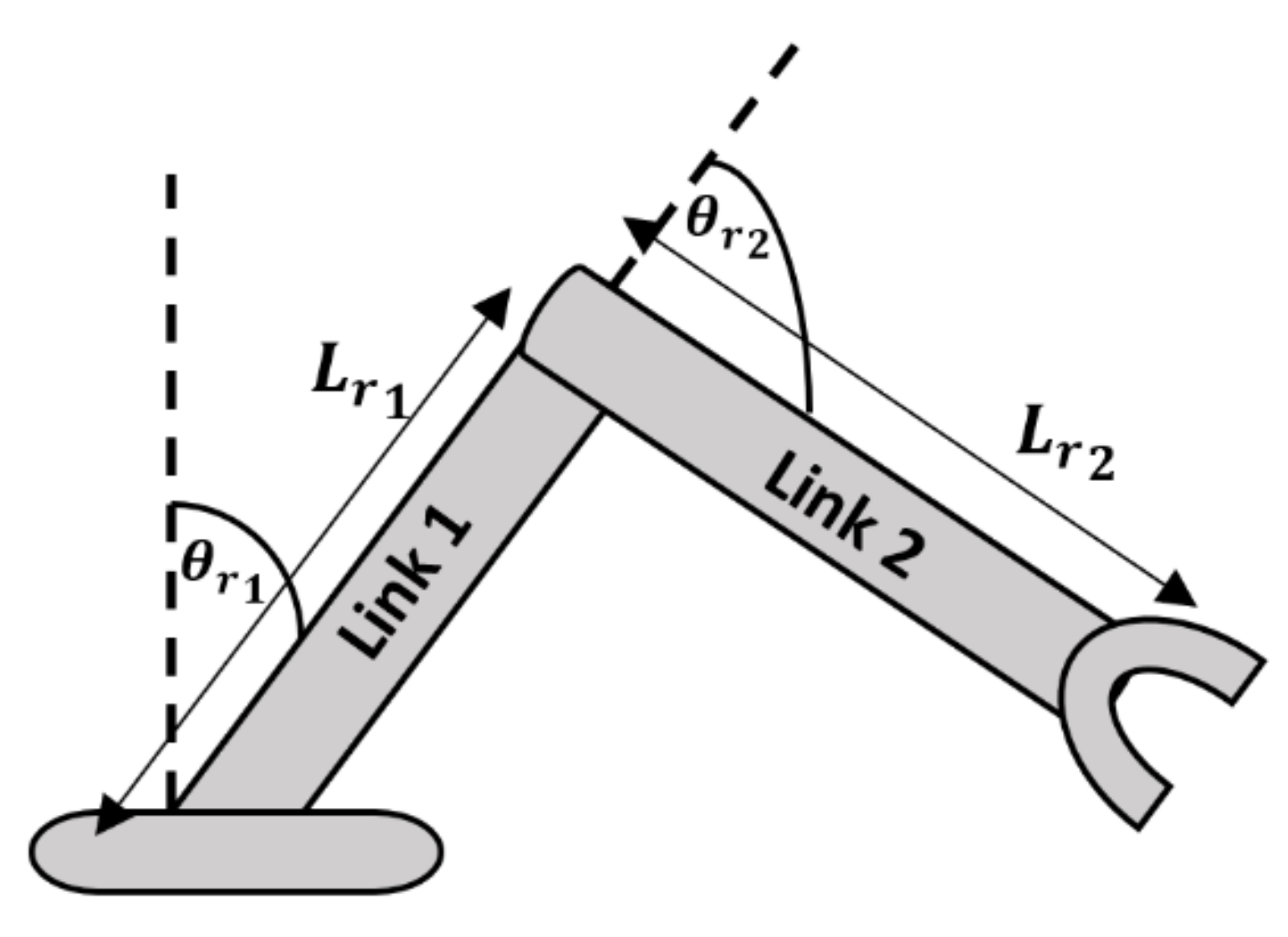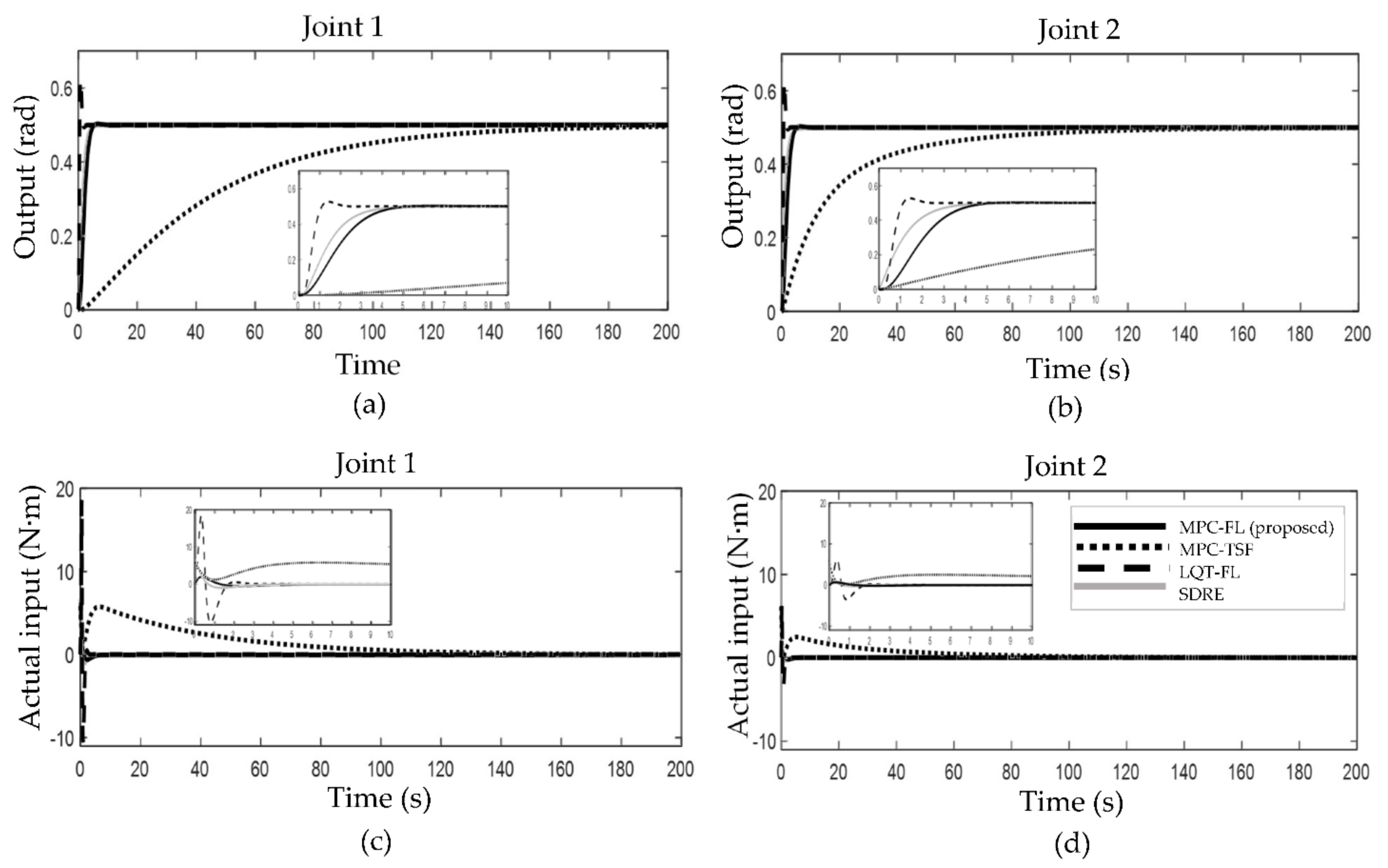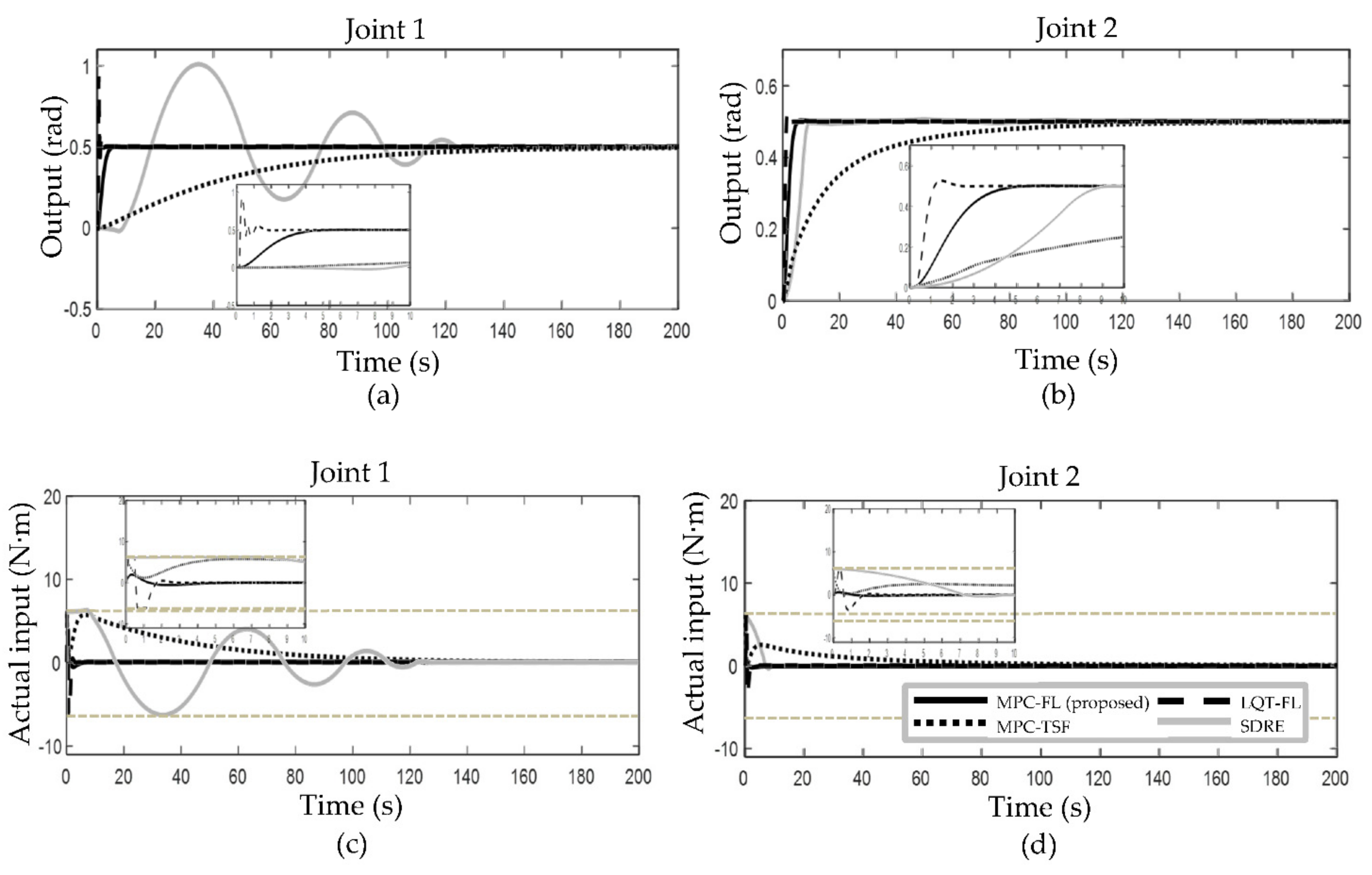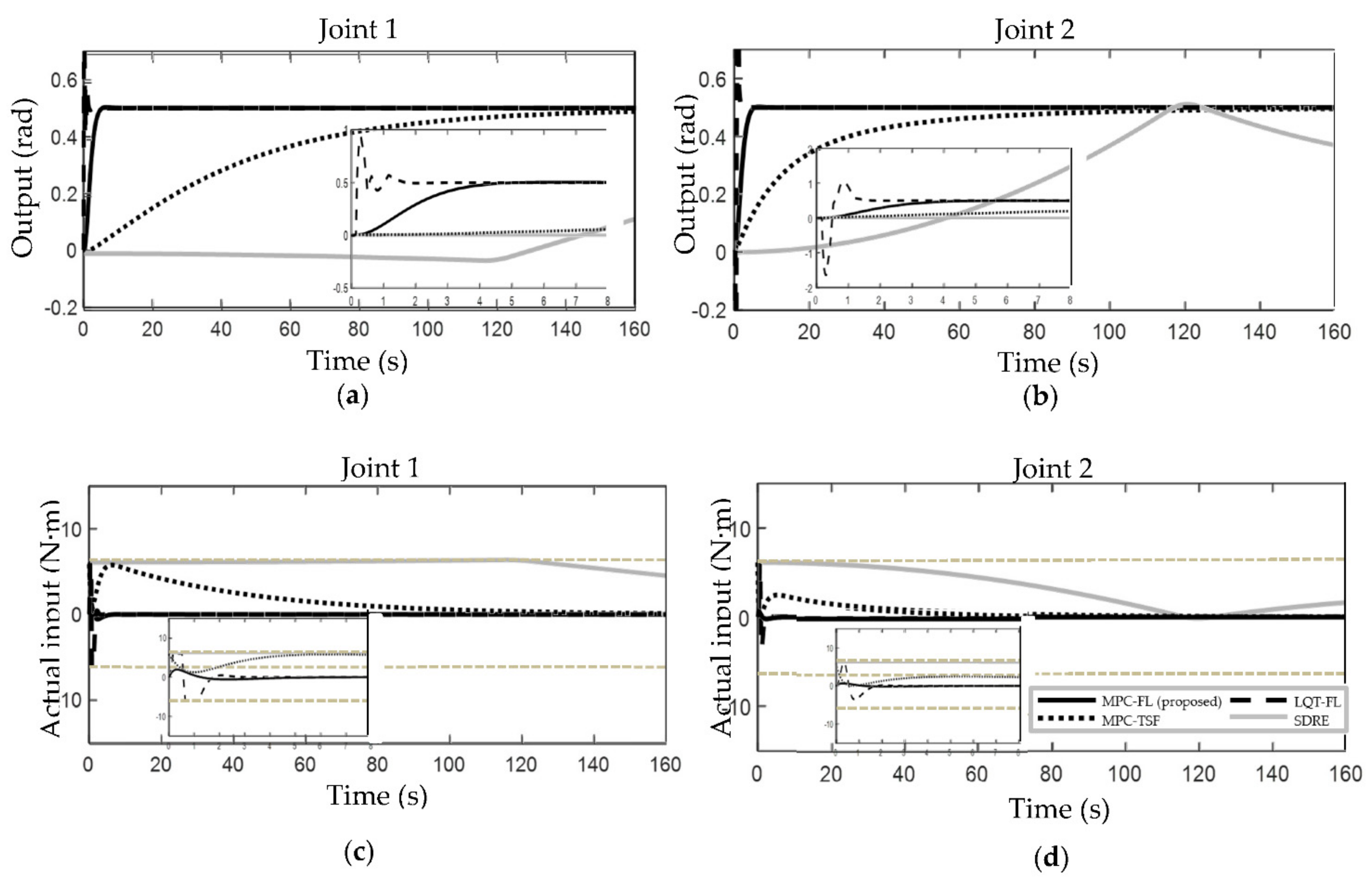Section 4 demonstrates two examples, the SISO and MIMO systems. Section 5 summarizes significant findings.

2. Linear or Linear-like Formulations of Nonlinear Systems

This section reviews some common techniques to transform a nonlinear system into a linear or linear-like system, which includes Jacobian linearization, feedback linearization, state-dependent coefficient (SDC) parameterization, and Takagi-Sugeno (T-S) fuzzy modeling.

A nonlinear system is considered as

$$\dot{\mathbf{x}}=\mathbf{f}\left(x\right)+\mathbf{g}\left(x\right)\mathbf{u}, \mathbf{y}=\mathbf{h}\left(x\right)$$

(1)

where $x$ is a state vector; $u$ is a control input vector; $\mathbf{y}$ is an output vector; $\mathbf{f}(x)$, $\mathbf{g}(x)$, and $\mathbf{h}(x)$ are nonlinear functions of the states and time.

The following subsection will present several schemes transforming Equation (1) into the linear or linear-like systems as the form:

$$\dot{z}=Az+Bv, w=Cz$$

(2)

where $z$, $v$ and $w$ are new state, control and output vectors, respectively; $A$, $B$ and $C$ are matrices derived from Equation (1). If they are not functions of $z$, Equation (2) is a linear system. In contrast, Equation (2) is linear-like system.

2.1. Jacobian Linearization

Jacobian linearization (JL) is a common approach, which uses a linear system to approximate a nonlinear system based on equilibrium points [19]. Thus, referring to Equation (2), the relevant variables are defined as

$$z=x-x_e,v=u, w=y-h(x_e), A={\left.\nabla f\right|}_{x=x_e}, B={\left.\nabla g\right|}_{x=x_e}, C={\left.\nabla h\right|}_{x=x_e}$$

(3)

where $x_e$ refers to equilibrium points. Since $A$, $B$ and $C$ are not functions of $z$, the obtained equation in Equation (2) is linear.

Since a nonlinear system might have multiple equilibrium points, each equilibrium point corresponds to a linear equation, such as Equation (2), which can be individually designed to have a controller. Thus, a common control scheme is called gain scheduling, and switches the controllers corresponding to different linear equations [20,21].

2.2. Feedback Linearization

Feedback linearization (FL) is a technique to algebraically transform a nonlinear to a linear system in another space by the exact transformation [22]. There are two types of FL which are the input-state and the input-output FL. They will be introduced below.

2.2.1. Input-State FL

One considers single-input nonlinear systems for input-state FL. To ensure that a linearization exists, both controllability and involutivity conditions should be satisfied. The linearization is performed based on a new state, where the first state can be determined by solving the equations [23]:

$$\nabla z_1{\mathrm{ad}}_f^{i}g=0 (i=0,\dots ,n-2), \nabla z_1{\mathrm{ad}}_f^{n-1}g\ne 0$$

(4)

where ${\mathrm{ad}}_f^{i}g$ is the adjoint representation of Lie algebra, and $n$ is the number of states.

Then, the new state $\mathbf{z}$ can be defined as

$$\mathbf{z}={[z_1\hspace{1em}{L}_{\mathbf{f}}{z}_1\hspace{1em}\dots \hspace{1em}{L}_{\mathbf{f}}^{n-1}{z}_1]}^T$$

(5)

where $L_{\mathbf{f}}{z}_1$ and $L_{\mathbf{f}}^{n-1}{z}_1$ are Lie derivatives.

Based on the new defined state $\mathbf{z}$, a linear system can be formulated as Equation (2), where:

$$A=\left[\begin{array}{lllll}0\hfill & 1\hfill & 0\hfill & \cdots \hfill & 0\hfill \\ 0\hfill & 0\hfill & 1\hfill & \cdots \hfill & 0\hfill \\ ⋮\hfill & ⋮\hfill & ⋮\hfill & \ddots \hfill & ⋮\hfill \\ 0\hfill & 0\hfill & 0\hfill & \cdots \hfill & 1\hfill \\ 0\hfill & 0\hfill & 0\hfill & \cdots \hfill & 0\hfill \end{array}\right], B=\left[\begin{array}{l}0\hfill \\ 0\hfill \\ ⋮\hfill \\ 0\hfill \\ 1\hfill \end{array}\right], v={\beta }^{-1}(u-\alpha )$$

(6)

in which

$$\alpha =-\frac{L_{\mathbf{f}}^n{z}_1}{L_g{L}_{\mathbf{f}}^{n-1}{z}_1}, \beta =\frac{1}{L_g{L}_{\mathbf{f}}^{n-1}{z}_1}$$

(7)

The input-state FL only transforms the state equation, so a linear output equation is not available. Besides, the obtained equation in Equation (2) is linear. For controller design, all linear control design schemes can be applied to have the control $v$, which can be transformed to the control $u$ by Equations (6) and (7), where $\beta$ cannot be zero.

2.2.2. Input-Output FL

One considers single-input-single-output nonlinear systems for input-output FL. The linearization is performed by differentiating the output equation in Equation (1) repeatedly until the input appears. Thus, the final equation will be [23]

$$y^{(r)}=L_{\mathbf{f}}^{r}h(x)+L_{\mathbf{g}}{L}_{\mathbf{f}}^{r-1}h(x)u$$

(8)

where $r$ is the number of differentiation and is called the relative degree of the system.

Define a new state $\mathbf{z}$ as

$$\mathbf{z}=[y\hspace{1em}\dot{y}\hspace{1em}\dots \hspace{1em}{y}^{(r-1)}{]}^T$$

(9)

Thus, Equation (8) can be formulated to be the same linear system as Equations (2) and (6), but the control $v$, the output $w$ and the parameter $C$ are written as

$$v=L_{\mathbf{f}}^{r}h(x)+L_g{L}_{\mathbf{f}}^{r-1}h(x)u, w=y, C=1$$

(10)

Similarly, the obtained equation in Equation (2) is linear. Besides, the control $v$ can be designed by all linear control schemes, and then the control $u$ can be determined by Equation (10), where $L_{\mathbf{g}}{L}_{\mathbf{f}}^{r-1}h(x)$ cannot be zero.

2.3. State Dependent Coefficient Parameterization

The state dependent coefficient (SDC) parameterization is a method that transforms a nonlinear to a linear-like system by factorizing the nonlinear functions [24]. Thus, Equation (1) can be rewritten as

$$\dot{\mathbf{x}}=\mathbf{f}\left(x\right)+\mathbf{g}\left(x\right)\mathbf{u}=\mathbf{A}(\mathbf{x})\mathbf{x}+\mathbf{B}(\mathbf{x})\mathbf{u}, \mathbf{y}=\mathbf{h}\left(x)=\mathbf{C}\right(x)x$$

(11)

where $\mathbf{f}\left(x\right)=\mathbf{A}(\mathbf{x})\mathbf{x}$, $\mathbf{g}\left(x\right)=\mathbf{B}(\mathbf{x})$, and $\mathbf{h}\left(x)=\mathbf{C}\right(\mathbf{x})x$.

Define the new state, control and output the same as the original ones:

$$z=x, v=u, w=y$$

(12)

which lead to the new state and output equations as Equation (2). Note that Equation (2) in this scheme is a set of linear-like equations. The major benefit of this scheme is design flexibility, but the stability and controllability it yields depend on the form of factorization.

Regarding control design, the state-dependent Riccati equation (SDRE) control is mostly applied to Equation (2). The design procedure of the control scheme is similar to the linear quadratic regulator (LQR), but the Riccati equations become functions of the states. This is the reason the control scheme is called the SDRE control, and the difficulty of the control scheme is solving the state-dependent Riccati equations.

2.4. Takagi–Sugeno Fuzzy Model

The Takagi–Sugeno fuzzy (TSF) model is a technique that locally linearizes a nonlinear system to linear subsystems. After that, fuzzy if-then rules are applied to choose and blend those linear subsystems for particular cases. The Takagi-Sugeno fuzzy models are given as [25]

The ith rule is expressed as

If ${\xi }_1$ is $M_{i1}$ and … and ${\xi }_q$ is $M_{iq}$, then

$$\dot{x}=A_{i}x+B_{i}u, y=C_{i}x, i=1,2,\cdots ,p$$

(13)

where ${\xi }_i$ are premise variables which are functions of the state variables; $M_{ij}$ is the fuzzy set; $p$ is the number of If-then rules; $q$ is the number of the premise variables; ${\mathbf{A}}_i$, ${\mathbf{B}}_i$, and ${\mathbf{C}}_i$ are state, input, and output matrices of the linear state-space of the ith rule.

Thus, the fuzzy systems are inferred as Equation (2), where:

$$A={\displaystyle \sum _{i=1}^p{h}_i(\mathsf{\xi })\cdot A_i}, B={\displaystyle \sum _{i=1}^p{h}_i(\mathsf{\xi })\cdot B_i}, C={\displaystyle \sum _{i=1}^p{h}_i(\mathsf{\xi })\cdot C_i}$$

(14)

in which

$$h_i(\mathsf{\xi })=({\displaystyle \prod _{j=1}^q{M}_{ij}})/({\displaystyle \sum _{i=1}^p{\displaystyle \prod _{j=1}^q{M}_{ij}}})$$

(15)

Note that the stability of the system is proved using Lyapunov function [26].

2.5. Comparisons of the Three Linear-like Structures

Jacobian linearization is based on Taylor’s series expansions, and only the first-order terms are remained. Thus, the transform systems are linear but approximate the original systems. The transformation is unique and is performed easily. The FL aims to have linear systems by defining new states and inputs. Thus, the transform systems present the original systems exactly, but the transformations of states and inputs are nonlinear and not unique. The non-unique property makes systems have design flexibilities for various applications. However, some conditions should be satisfied. The state dependent coefficient parameterization seeks a linear-like form, which can be directly applied by linear control theorems. This expression is exactly the same as the original one, but the state, input and output matrices become state-dependent. This transformation is not unique, and some conditions should be satisfied. For instance, the determinant of the state matrix cannot be infinite at any instant. The TSF models try to have a set of locally linear subsystems to express the original systems by imposing a set of membership functions. However, the new systems are approximately linear-like, due to state-dependent membership functions.

Table 1. Comparisons of the four transformations.

Transformation Schemes	JL	FL	SDC Parameterization	TSF Model
Redefine states and inputs	N	Y	N	N
Linear or linear-like	Linear	Linear	Linear-like	Linear-like
Approximated or same representations	Approximated	Same	Same	Approximated
Condition satisfied	N	Y	Y	N
Design flexibility	N	Y	Y	Y
Formulation complexity	N	Y	N	Y
Computation cost	Low	Low	High	High

lists the comparisons of these schemes.

3. Nonlinear Model Predictive Control Formulation

This section presents a nonlinear model predictive tracking control with input constraints based on FL, where Laguerre functions are applied to reduce computation burdens, and the formulated control problem is solved by using Hildreth’s quadratic programming [27]. The detailed formulations are presented as follows.

3.1. Problem Description

Consider a nonlinear system as Equation (1) with input constraints as

$${\mathbf{u}}^{-}\le \mathbf{u}\le {\mathbf{u}}^{+}$$

(16)

where ${\mathbf{u}}^{-}$ and ${\mathbf{u}}^{+}$ are the lower and upper bounds of the inputs.

By performing FL as shown in Section 2.2, a nonlinear system in Equation (1) with the input constraints in Equation (16) can be transformed as Equation (2) with the new input constraints as

$$v^{-}\le v\le v^{+}$$

(17)

where $v^{-}$ and $v^{+}$ are the new lower and upper bounds of the new inputs, which are obtained through Equation (6).

3.2. Laguerre Functions

The Laguerre functions are the set of the orthonormal basis functions, and they will be used to approximate the control signals to decrease the computational time of the model predictive control [28,29]. The set of Laguerre functions can be arranged in the matrix form as

$$L(t)=e^{{\mathbf{A}}_{l}t}\mathbf{L}\left(0\right)$$

(18)

where:

$$A_l={\left[\begin{array}{cccc}-p& 0& \cdots & 0\\ -2p& -p& \cdots & 0\\ ⋮& ⋮& \ddots & ⋮\\ -2p& \cdots & -2p& -p\end{array}\right]}_{N\times N},\hspace{1em}L(0)=\sqrt{2p}{\left[\begin{array}{c}1\\ 1\\ ⋮\\ 1\end{array}\right]}_{N\times 1}, p>0$$

(19)

in which $p$ is a scaling factor which implies the exponential decay rate; $N$ is the number of coefficients. As $N$ increases, the estimated input signal is closer to the real value. Figure 1 shows an input signal approximated by using the Laguerre functions. It is worth to note that the Laguerre functions have the property of orthonormality.

3.3. Model Predictive Control with Input Constraints

The MPC computes a control signal by optimizing the outputs based on a predicted model within a limited time window. Thus, the MPC can be formulated as an optimization problem subjected to some constraints, and the MPC formulations are shown as follows.

Define a new state as

$$\mathsf{\chi }=[{\dot{\mathbf{z}}}^T\hspace{1em}{e}^T{]}^T$$

(20)

where $\mathbf{e}$ is the tracking error defined as

$$\mathbf{e}=\mathbf{y}-{\mathbf{r}}_f$$

(21)

in which ${\mathbf{r}}_f$ is a constant reference signal to be tracked by the output $\mathbf{y}$.

Taking the derivative of the state-space equation in Equation (2) with respect to time leads to

$$\ddot{z}=A\dot{z}+B\dot{v}$$

(22)

Also, the time derivative of Equation (21) leads to

$$\dot{\mathbf{e}}=\dot{\mathbf{y}}=\mathbf{C}\dot{\mathbf{z}}$$

(23)

Based on the definition of the new state shown in Equation (20), combining Equations (22) and (23) become to the augmented model as

$$\dot{\mathsf{\chi }}={\mathbf{A}}_g\mathsf{\chi }+{\mathbf{B}}_g\dot{\mathbf{v}}, e=C_g\mathsf{\chi }$$

(24)

where:

$${\mathbf{A}}_g=\left[\begin{array}{cc}\mathbf{A}& {\mathbf{0}}_{n_{out}\times n_{state}}^T\\ \mathbf{C}& {\mathbf{0}}_{n_{out}\times n_{out}}\end{array}\right], {\mathbf{B}}_g=\left[\begin{array}{c}B\\ {\mathbf{0}}_{n_{out}\times n_{in}}\end{array}\right], C_g=[\begin{array}{cc}{0}_{n_{out}\times n_{state}}& I_{n_{out}\times n_{out}}\end{array}]$$

(25)

in which $n_{in}$, $n_{out}$ and $n_{state}$ are the numbers of inputs, outputs and states, respectively.

Therefore, the MPC optimization problem can be formulated as [29]

$$\mathrm{Min} J={\displaystyle {\int }_0^{T_p}({\mathsf{\chi }}^T(t_i+\tau )\mathbf{Q}\mathsf{\chi }(t_i+\tau )+{\dot{\mathbf{v}}}^T(\tau )\mathbf{R}\dot{\mathbf{v}}(\tau ))d\tau }$$

(26)

subjected to the augmented equations as (24) and the input constraints as (17), where $t_i$ is the current time in the model predictive control; $T_p$ is the time of horizon window; $\mathbf{Q}$ and $\mathbf{R}$ are the weighting diagonal matrices for state and input, respectively.

The Laguerre functions are applied to estimate the control signal expressed as

$${\dot{v}}_i(t)={\mathbf{L}}_i{}^T(t){\mathsf{\eta }}_i$$

(27)

where $v_i(t)$ is the ith control signal in vector $v(t)$; ${\mathbf{L}}_i(t)$ and ${\mathsf{\eta }}_i$ are two $(N_i\times 1)$ vectors associated with the control $v_i(t)$, and $N_i$ is the number of the Laguerre functions regarding to the ith control $v_i(t)$.

Since the Laguerre functions have the property of the orthonormality, Equation (27) substituted into (17) and (24) leads to

$$\overline{\mathbf{M}}\mathsf{\eta }\le \overline{\mathsf{\gamma }}$$

(28)

$$\mathsf{\chi }(t_i+\tau )=e^{{\mathbf{A}}_g\tau }\mathsf{\chi }(t_i)+{\mathsf{\varphi }}^T(\tau )\mathsf{\eta }$$

(29)

where $\eta$ is a vector consisting all ${\mathsf{\eta }}_i$, and

$$\overline{\mathbf{M}}=\left[\begin{array}{c}diag(L_1^T(0)\Delta t,L_2^T(0)\Delta t,\cdots ,L_{n_{in}}^T(0)\Delta t\\ diag(-L_1^T(0)\Delta t,-L_2^T(0)\Delta t,\cdots ,-L_{n_{in}}^T(0)\Delta t\end{array}\right]$$

(30)

$$\overline{\mathsf{\gamma }}={\left[v_{{}_1}^{+}-v_1(t_i-\mathsf{\Delta }t)\hspace{1em}-v_{{}_1}^{-}+v_1(t_i-\mathsf{\Delta }t)\hspace{1em}\cdots \hspace{1em}{v}_{{}_{n_{in}}}^{+}-v_{n_{in}}(t_i-\mathsf{\Delta }t)\hspace{1em}-v_{{}_{n_{in}}}^{-}+v_{n_{in}}(t_i-\mathsf{\Delta }t)\right]}^T$$

(31)

$${\mathsf{\varphi }}^T(\tau )={\displaystyle {\int }_0^{\tau }{e}^{{\mathbf{A}}_g(\tau -\gamma )}\left[{\mathbf{B}}_1{\mathbf{L}}_1{}^T(\gamma )\hspace{1em}{\mathbf{B}}_2{\mathbf{L}}_2{}^T(\gamma )\hspace{1em}\dots \hspace{1em}{\mathbf{B}}_{n_{in}}{\mathbf{L}}_{n_{in}}{}^T(\gamma )\right]d\gamma }$$

(32)

in which ${\mathbf{B}}_i$ is the ith column of the ${\mathbf{B}}_g$ matrix and $\tau$ is the time between 0 and $T_p$.

The equality constraint shown in Equation (29) can be substituted into (26) to eliminate a constraint in the optimization problem, and it can be reformulated as

$$\begin{gathered} \min J={[\mathsf{\eta }+{\mathsf{\Omega }}^{-1}\mathsf{\Psi }\mathsf{\chi }(t_i)]}^T\Omega [\eta +{\Omega }^{-1}\Psi \chi (t_i)] \\ +{\mathsf{\chi }}^T(t_i)({\displaystyle {\int }_0^{T_p}{e}^{A_g^T\tau }\mathbf{Q}{e}^{A_g\tau }d\tau })\mathsf{\chi }(t_i)-{\mathsf{\chi }}^T(t_i){\Psi }^T{\Omega }^{-1}\mathsf{\Psi }\mathsf{\chi }(t_i) \end{gathered}$$

(33)

subjected to Equation (28), where:

$$\mathsf{\Omega }={\displaystyle {\int }_0^{T_p}\mathsf{\varphi }(\tau )\mathbf{Q}{\mathsf{\varphi }}^T(\tau )d\tau }+{\mathbf{R}}_L, \mathsf{\Psi }={\displaystyle {\int }_0^{T_p}\mathsf{\varphi }(\tau )\mathbf{Q}{e}^{{\mathbf{A}}_g\tau }d\tau }$$

(34)

The optimization problem can be solved by using the Hildreth’s quadratic programming [27] to obtain

$$\mathsf{\eta }=-{\mathsf{\Omega }}^{-1}\mathsf{\Psi }\mathsf{\chi }-{\mathsf{\Omega }}^{-1}{\overline{\mathbf{M}}}^T\mathsf{\lambda }$$

(35)

where:

$$\mathsf{\lambda }=\left[{\mathsf{\lambda }}_1\hspace{1em}\cdots \hspace{1em}{\mathsf{\lambda }}_i\right], i=1,2,\dots ,2n_{in}$$

(36)

which can be obtained by

$${\lambda }_i^{m+1}=\max \left(0,{\mathsf{\Lambda }}_i^{m+1}\right), m=1,2,\dots ,n_{cons}$$

(37)

where $n_{cons}$ is the number of input constraints, and

$${\mathsf{\Lambda }}_i^{m+1}\left(t\right)=-\frac{1}{H_{ii}}\left[K_i+{\displaystyle \sum }_{j=1}^{i-1}{H}_{ij}{\lambda }_j^{m+1}\left(t\right)+{\displaystyle \sum }_{j=i+1}^{n_{cons}}{H}_{ij}{\lambda }_j^m\left(t\right)\right]$$

(38)

in which $K_i$ and $H_{ij}$ are the components of matrices

$$\mathbf{K}=\overline{\mathsf{\gamma }}+\overline{\mathbf{M}}{\mathsf{\Omega }}^{-1}\mathsf{\Psi }\mathsf{\chi }, \mathbf{H}=\overline{\mathbf{M}}{\mathsf{\Omega }}^{-1}{\overline{\mathbf{M}}}^T$$

(39)

Thus, the new control $\dot{v}$ is obtained through Equation (27), where the vector $\mathsf{\eta }$ is calculated by using Equation (35). The vector $\mathsf{\eta }$ is in terms of the vector $\mathsf{\lambda }$, which is determined by Equation (37). Each element in vector $\mathsf{\lambda }$ is either zero or positive values, which refer to non-active or active constraints, respectively. If there are no active constraints, $\mathsf{\lambda }$ will contain only zero and the control $\dot{v}$ can be expressed as

$$\dot{\mathbf{v}}=-{\mathbf{K}}_{MPC}\mathsf{\chi }$$

(40)

where:

$${\mathbf{K}}_{MPC}={\mathbf{L}}^T(0){\mathsf{\Omega }}^{-1}\mathsf{\Psi }$$

(41)

The proposed approach is flexible for control design, because there are five controller parameters tuned to enhance control performances. The five parameters are the scaling factor $p$, the numbers of the Laguerre functions $N_i$ regarding to the ith control, the time of horizon window $T_p$, and the weighting matrices $\mathbf{Q}$ and $\mathbf{R}$ respectively for the augmented states and the new control rates. The scaling factor is the decaying rate of the Laguerre functions, which affect the approximations of the control rates. The more the numbers of the Laguerre functions are, the closer the approximated control rates are to the real ones, but the penalty is the computational cost. If the time of horizon window approaches infinity, the model predictive control is similar as the LQR control. Obviously, the weight matrices affect the minimizations of the augmented states and the new control rates. From the perspective of practical control, the parameter tuning procedure is summarized as follows.

• Select the scaling factor, which is related to the convergence rates of the Laguerre functions. Equation (18) can be used to test the convergence rates by selecting various scaling factor. It is suggested that a trial starts from $p=1$.
• Select the numbers of the Laguerre functions, which are related the approximation accuracy of control signals. Using more Laguerre functions causes better approximates but more computational time. It is suggested that a trial starts from $N_i=3$.
• Select the time of horizon window, which is related to the time to predict the response. There are no general rules to select the time, but it is suggested that a trial starts from $T_p=100$.
• Select the weighting matrices, which are related to the minimizations of the states and control. Since they are usually contradictive, it is suggested that a trial starts from $\mathbf{Q}=\mathbf{R}=\mathbf{I}$.
• After performing the first trials, all parameters can be adjusted by several trials based on the trial results.

4. Illustrative Examples

This section demonstrates two examples: a flexible-joint mechanism and a two-link robot arm, which are a single-input single-output system (SISO) and as a multiple-input multiple-output system (MIMO), respectively. To demonstrate the control performances, the three control schemes in literature listed below are applied to compare their simulation results.

• Linear quadratic tracking (LQT) control based on FL: this scheme applies the input-state FL shown in Section 2.2.1. first, and then the LQT control is applied to design a control. This scheme is abbreviated as LQT-FL in the following simulations.
• MPC based on the TSF model: this scheme applied the TSF model to obtain a linear-like model first, and then the MPC is used to design the control. This scheme is abbreviated as MPC-TSF in the following simulations.
• SDRE control: this scheme applies the SDC parameterization shown in Section 2.3. to nonlinear systems first, and then the control is obtained by solving the SDRE. The control design process is similar to the LQR control, so this scheme is like an LQR based on the SDC. In this study, this scheme is abbreviated as SDRE in the following simulations.

As a matter of fact, the proposed scheme applied the input-state FL first, and then the MPC is used to design a control. Thus, the proposed scheme is abbreviated as MPC-FL in the following simulations. Obviously, the proposed scheme is compared with the MPC-TSF to show the effects of the linearized-like scheme; the proposed scheme is compared with the LQT-FL to show the effects of control designs; the proposed scheme is compared with the SDRE to show both the effects of linearized-like schemes and control designs. Note that a saturation function is applied to the three compared control schemes in order to satisfy the input constraints.

4.1. Flexible-Joint Mechanism

The dynamics model of the flexible-joint mechanism, shown in Figure 2, is given by

$$I_m{\ddot{q}}_{m_1}+M_{m}g{L}_m\sin q_{m_1}+K_m(q_{m_1}-q_{m_2})=0, J_m{\ddot{q}}_{m_2}-K_m(q_{m_1}-q_{m_2})=u_m$$

(42)

where $u_m$ is the motor torque defined as the input signal; $q_{m_1}$ is the angular displacement of the joint attached with the link defined as the output signal; $q_{m_2}$ is the angular displacement of the joint attached with the motor.

To perform the tracking control, one intends the angle $q_{m_1}$ to reach 0.6 rad by applying the aforementioned four control schemes. The parameters applied in the simulation are defined in

Table 2. Parameters of the flexible-joint mechanism.

Parameters	Symbols	Values	Units
Inertia of the link	$I_m$	1	kg⋅m2
Inertia of the motor	$J_m$	1	kg⋅m2
Mass of the link	$M_m$	1	kg
Distance between the joint and the link center	$L_m$	1	m
Spring constant	$K_m$	100	N/rad
Gravitational constant	$g$	9.81	m/s2

, and the controller parameters are selected as

$$p=0.5, N=5, T_p=100, \mathbf{Q}=\mathbf{I}, r=1$$

(43)

For comparisons, the controller parameters of the other three schemes are selected as

$$\mathrm{SDRE}: \mathbf{Q}=\mathbf{I}, r=1$$

(44)

$$\text{MPC-TSF}: p=0.5, N=5, T_p=100, \mathbf{Q}=\mathbf{I}, r=1$$

(45)

$$\text{LQT-FL}: \mathbf{Q}=\mathbf{I}, r=1$$

(46)

Note that the controller parameter values are the same in the four control schemes.

Case A: Control without input constraints for the flexible-joint mechanism

Figure 3a shows the output responses by applying the four control schemes without input constraints. The results show that the responses of the SDRE and LQT-FL have overshoots and oscillations. In contrast, the proposed control MPC-FL and the MPC-TSF model provide smooth responses. Moreover, the proposed control has the smallest settling time, compared with the other three control schemes. Figure 3b shows the control signals by applying the four control schemes without input constraints, and the results show that the proposed control MPC-FL and the MPC-TSF have smoother and smaller control signals, compared with the other two control schemes.

Table 3. Performance comparisons of applying the four control schemes to the flexible-joint mechanism without input constraints.

Controller	Rising Time (s)	Settling Time (s)	Max. Overshoot (Rad)	Input Ranges (N·m)	Computational Time (s)	RMSE (Rad)
SDRE	1.1120	15.8700	0.3589	(−1.9091, 0.9438)	43.0110	0.0688
MPC-TSF	13.3184	20.1470	0.0002	(−0.0004, 0.5991)	45.0750	0.1333
LQT-FL	6.1280	48.8000	0.4638	(−4.9458, 5.5785)	1.5310	0.1918
MPC-FL (proposed)	9.2668	12.6885	0.0000	(−0.0004, 1.0480)	15.5830	0.1564

shows the control performance comparisons by applying the four control schemes, where there are six performances indices selected for comparisons, which are the rising time, the settling time, the maximum overshoots, the ranges of input signals, the computational time, and the root-mean square errors (RMSEs). The results show that the smallest rising and settling come from the LQT-FL and the proposed MPC-FL, respectively; the proposed MPC-FL provides the smallest and near-zero overshoots; the MPC-TSF provides the smallest range of input signals; the LQT-FL takes the shortest computational time; the MPC-TSF provides the smallest RMSE. Although the proposed control scheme has only two first places in the six performance indices, the scheme has the other four second places. Therefore, speaking overall, the proposed scheme is superior to the other schemes in this example.

Case B: Control with input constraints for the flexible-joint mechanism

Similar simulations are performed in this case, except for the control with input constraints. To test the capability of enduring input constraint ranges, the range starts from a bigger value and is then followed by smaller values. One selects the input constraints as ±4.5, ±1.9, ±1.8, ±0.59, and ±0.56, and Figure 4, Figure 5, Figure 6, Figure 7 and Figure 8 show the output response and the input signals associated with the constraints, respectively. Regarding the input constraints ±4.5, the constraints are active only for the LQT-FL, but the response has huge overshoots. Regarding the input constraints ±1.9, the constraints are active for the LQT-FL and SDRE. Although both can reach the desired angle, the LQT-FL has huge overshoots. Regarding the input constraints ±1.8, the constraints are active for the LQT-FL and SDRE, where the LQT-FL has not only huge overshoots but also fluctuations at the steady state, while the SDRE cannot track the reference signal. Regarding the input constraints ±0.59, the constraints are active for all controllers, where only the LQT-FL, MPC-TSF and proposed MPC-FL can track the reference signal, but the LQT-FL has huge overshoots and the MPC-TSF has a longer settling time, compared with the proposed MPC-FL. Regarding the input constraints ±0.56, the constraints are active for all controllers but only the proposed MPC-FL and LQT-FL could track the reference signal effectively, although the LQT-FL still has huge overshoots.

Table 4. Comparisons of control performances by applying the four control schemes with input constraints to the flexible-joint mechanism.

Input Constraints (N⋅m)	Controllers	Rising Time (s)	Settling Time (s)	Max. Overshoot (Rad)	RMSE (Rad)
±4.5	SDRE	1.1120	15.8700	0.3589	0.0688
	MPC-TSF	13.3184	20.1470	0.0002	0.1333
	LQT-FL	N/A	44.7200	N/A	N/A
	MPC-FL (proposed)	9.2668	12.6885	0.0000	0.1564
±1.9	SDRE	1.1360	18.7600	0.3588	0.0766
	MPC-TSF	13.3184	20.1470	0.0002	0.1333
	LQT-FL	N/A	45.7200	N/A	N/A
	MPC-FL (proposed)	9.2668	12.6885	0.0000	0.1564
±1.8	SDRE	0.7194	N/A	0.3500	0.1324
	MPC-TSF	13.3184	20.1470	0.0002	0.1333
	LQT-FL	N/A	46.7000	N/A	N/A
	MPC-FL (proposed)	9.2668	12.6885	0.0000	0.1564
±0.59	SDRE	N/A	N/A	N/A	N/A
	MPC-TSF	13.6132	23.2655	0.0000	0.1334
	LQT-FL	N/A	47.4700	N/A	N/A
	MPC-FL (proposed)	15.0869	20.5160	0.0000	0.1807
±0.56	SDRE	N/A	N/A	N/A	N/A
	MPC-TSF	N/A	N/A	N/A	N/A
	LQT-FL	N/A	50.3700	N/A	N/A
	MPC-FL (proposed)	15.3072	20.5160	0.0000	0.1840

Note: N/A refers to the values much greater than the others or non-existent.

shows the performance indices, which are the rising time, the settling time, the maximum overshoots, the ranges of input signals, and the RMSEs. The results show that a larger input constraint range can be satisfied by all control schemes. However, as the range increases, some control schemes may not track the reference signal. Even though some of them track the signal effectively, the performance indices are worse than those obtained by the proposed MPC-FL.

4.2. Two-Link Robot Arm

The dynamics model of the system is (shown in Figure 9) given by

$${\mathbf{M}}_r({\mathsf{\theta }}_r){\ddot{\mathsf{\theta }}}_r+{\mathbf{C}}_r({\mathsf{\theta }}_r,{\dot{\mathsf{\theta }}}_r)={\mathbf{u}}_r$$

(47)

where ${\mathsf{\theta }}_r$ and $u_r$ are vectors of the link angles and applied torques, respectively; $M_r({\mathsf{\theta }}_r)$ is a mass matrix function of ${\mathsf{\theta }}_r$ and $C_r({\mathsf{\theta }}_r,{\dot{\mathsf{\theta }}}_r)$ is a Coriolis force vector function of ${\mathsf{\theta }}_r$ and ${\dot{\mathsf{\theta }}}_r$, and both are given as

$$\begin{gathered} {\mathbf{M}}_r\left({\mathsf{\theta }}_r\right)=\left[\begin{array}{cc}(m_{r_1}+m_{r_2})L_{r_1}^2+m_{r_2}{L}_{r_2}^2+2m_{r_2}{L}_{r_1}{L}_{r_2}\cos {\theta }_{r_2}& m_{r_2}{L}_{r_2}^2+m_{r_2}{L}_{r_1}{L}_{r_2}\cos {\theta }_{r_2}\\ m_{r_2}{L}_{r_2}^2+m_{r_2}{L}_{r_1}{L}_{r_2}\cos {\theta }_{r_2}& m_{r_2}{L}_{r_2}^2\end{array}\right], \\ {\mathbf{C}}_r({\mathsf{\theta }}_r,{\dot{\mathsf{\theta }}}_r)=\left[\begin{array}{c}-m_{r_2}{L}_{r_1}{L}_{r_2}(2{\dot{\theta }}_{r_1}{\dot{\theta }}_{r_2}+{\dot{\theta }}_{r_1}{}^2)\sin {\theta }_{r_2}\\ -m_{r_2}{L}_{r_1}{L}_{r_2}{\dot{\theta }}_{r_1}{\dot{\theta }}_{r_2}\sin {\theta }_{r_2}\end{array}\right] \end{gathered}$$

(48)

in which $m_{r_1}$ and $m_{r_2}$ are the masses of links; $L_{r_1}$ and $L_{r_2}$ are the lengths of links; ${\theta }_{r_1}$ and ${\theta }_{r_2}$ are the joint angles; the subscripts 1 and 2 refer to the first and second links, respectively.

In this study, the joint torques are the control inputs, and the joint angles are the outputs. Thus, this system has two inputs and two outputs. The system parameters are shown in Table 5. The tracking control is performed to track the reference signals 0.5 for both joints. Similar to the previous example, the four control schemes were applied to compare their control performances. The robot parameters are listed in Table 4, and the controller parameters are given as

$$Q=150I, R=I, p=0.9, N=7, T_p=15$$

(49)

For comparisons, the controller parameters of the other three schemes are selected as

$$\mathrm{SDRE}: Q=150I, R=I$$

(50)

$$\text{MPC-TSF}: Q=150I\mathbf{,} R=I\mathbf{,} p=0.9, N=7, T_p=15$$

(51)

$$\text{LQT-FL}: Q=150I, R=I$$

(52)

Note that the controller parameter values are the same in the four control schemes.

Table 5. Two-link robot arm parameters.

Parameters	Symbols	Values	Units
Mass of link 1	$m_{r_1}$	1	kg
Mass of link 2	$m_{r_2}$	0.5	kg
Length of link 1	$L_{r_1}$	1	m
Length of link 2	$L_{r_2}$	0.8	m

Table 5. Two-link robot arm parameters.

Parameters	Symbols	Values	Units
Mass of link 1	$m_{r_1}$	1	kg
Mass of link 2	$m_{r_2}$	0.5	kg
Length of link 1	$L_{r_1}$	1	m
Length of link 2	$L_{r_2}$	0.8	m

Case C: Control without the input constraints for the two-link robot arm

Figure 10 shows the output and input responses by applying the control schemes. The results show that all schemes can track the reference signals but the response of the MPC-TSF is much slower than that of the other schemes. To distinguish the three schemes, Figure 11 shows their transients, and the results show that the overshoot of the LQT-FL is greater than those of the other two schemes.

Table 6. Comparisons of control performances by applying the four control schemes without input constraints to the two-link robot arm.

Controller	Joint	Rising Time (s)	Settling Time (s)	Max. Overshoot (Rad)	Input Ranges (N·m)	Computational Time (s)	RMSE (Rad)
SDRE	1	4.4800	6.6400	0.0000	(−0.9893, 6.4839)	167.4830	0.3419
	2	4.3040	5.8200	0.0000	(−0.3345, 6.1237)		0.2807
MPC-TSF	1	110.7220	147.5750	0.0000	(0.0000, 5.8805)	39.4840	0.1776
	2	107.8150	137.2700	0.0000	(0.0000, 6.1647)		0.1045
LQT-FL	1	1.1840	2.4400	0.0250	(−10.4705, 18.5682)	6.4400	0.2572
	2	1.1360	2.4100	0.0260	(−3.5592, 6.3192)		0.2543
MPC-FL (proposed)	1	3.9240	5.4250	0.0028	(−0.5592, 1.9739)	6.5200	0.0409
	2	3.7480	5.3320	0.0028	(−0.1901, 0.6711)		0.0407

shows the control performances by applying the four control schemes. The results show that the LQT-FL has the smallest rising and settling time. The SDRE and MPC-TSF have near-zero overshoots, and the overshoot of the proposed MPC-FL is smaller than that of the MPC-TSF. The proposed MPC-FL has the smallest input range, which implies that its control effort is smallest. The RMSEs of the proposed MPC-FL are smallest. Speaking overall, the proposed MPC-FL has the first or second places in the six performance indices, and its performances are better than others in this case.

Case D: Control with the input constraints for the two-link robot arm.

Similar to case C, one reduces the input constraint range to test the capabilities of enduring the minimum range, and the ranges are selected as ±6.1, ±6.0, and ±1.5/±0.3 N⋅m for both joints. Regarding the range ±6.1 N⋅m for both joints, the results are shown in Figure 11. The results show that all control schemes can track the reference signals, where the input constraints for the MPC-TSF, LQT-FL, and SDRE are active. Besides this, the proposed MPC-FL converges faster than the others, and it has smaller overshoot. Regarding the range ±6.0 N⋅m for both joints, the results are shown in Figure 12. Although the range is a little smaller than the previous range, the results are much different. The results show that the input constraints for all control schemes are active, but the SDRE cannot track the reference signals in contrast to other control schemes. Furthermore, the proposed MPC-FL has less rising and settling time. Regarding the range ±1.5/±0.3⋅m for each joint, the results are shown in Figure 13. The results show that the input constraints of all control schemes are active, so the input signals reach the constraint bounds. Besides this, the output signals of the SDRE and MPC-TSF cannot track the reference signals, and the proposed MPC-FL has smaller overshoot.

Table 7. Comparisons of control performances by applying the four control schemes with input constraints to the two-link robot arm.

Input Constraint Range (N⋅m)	Controllers	Joints	Rising Time (s)	Settling Time (s)	Max. Overshoot (Rad)	RMSE (Rad)
±6.1	SDRE	1	28.1920	127.3500	0.5094	0.5005
		2	7.8480	10.6800	0.0059	0.4903
	MPC-TSF	1	110.4480	138.7900	0.0000	0.1884
		2	88.1920	119.3350	0.0000	0.1253
	LQT-FL	1	0.2560	2.0900	0.4310	0.1785
		2	0.6720	2.0200	0.0327	0.6997
	MPC-FL (proposed)	1	3.9240	5.4250	0.0028	0.0409
		2	3.7480	5.3320	0.0028	0.0407
±6.0	SDRE	1	N/A	N/A	N/A	N/A
		2	N/A	N/A	N/A	N/A
	MPC-TSF	1	125.3890	156.7362	0.0000	0.4993
		2	104.8225	131.0281	0.0000	0.4740
	LQT-FL	1	0.2160	2.3000	0.4383	0.1789
		2	0.6640	2.1300	0.5421	0.7034
	MPC-FL (proposed)	1	3.9240	5.4250	0.0028	0.0409
		2	3.7480	5.3320	0.0028	0.0407
±1.5/±0.3	SDRE	1	N/A	N/A	N/A	N/A
		2	N/A	N/A	N/A	N/A
	MPC-TSF	1	N/A	N/A	N/A	N/A
		2	N/A	N/A	N/A	N/A
	LQT-FL	1	0.8480	2.1700	0.0379	0.1539
		2	0.0560	1.6700	0.9551	0.1528
	MPC-FL (proposed)	1	3.5800	5.4100	0.0028	0.0409
		2	4.1360	5.6600	0.0031	0.0567

Note: N/A refers to the values much greater than the others or non-existent.

summarizes the performance indices with the three input constraint ranges, and the results show that the LQT-FL has the smallest rising and settling time, and the proposed MPC-FL has the smallest ranges of inputs and RMSE.

5. Conclusions

This paper presents a continuous-time model predictive tracking control, based on input-state feedback linearization for nonlinear systems with input constraints. Although literature shows some similar control schemes, their formulations are quite complex and they need high computational costs. To reduce formulation complexities and computational loads, this study considers the control signals to be approximated with Laguerre functions, and the control problem is formulated as a constrained quadratic optimization problem solved by the Hildreth’s quadratic programming procedure. Since the proposed control is based on linear systems, which are obtained through feedback linearization, this study also investigates the effects of linearization or linearization-like effects. The relevant developed schemes include not only feedback linearization but also Jacobian linearization, state-dependent factorization, and the Takagi–Sugeno fuzzy model. Based on these schemes integrated in the model predictive control, the linear quadratic tracking control, and the state-dependent Riccati method control, the proposed control is applied to two nonlinear systems to demonstrate it controls performances, and the results show that the proposed control is superior to the others.

References

1. Schwenzer, M.; Ay, M.; Bergs, T.; Abel, D. Review on model predictive control: An engineering perspective. Int. J. Adv. Manuf. Technol. 2021, 117, 1327–1349. [Google Scholar] [CrossRef]
2. Camacho, E.F.; Alba, C.B. Model Predictive Control; Springer: Berlin/Heidelberg, Germany, 2013. [Google Scholar]
3. Baillieul, J.B.; Willems, J.C.; Mitter, S.K. Mathematical Control Theory; Springer: Berlin/Heidelberg, Germany, 1999. [Google Scholar]
4. Kurtz, M.J.; Henson, M.A. Input-output linearizing control of constrained nonlinear processes. J. Process Control 1997, 7, 3–17. [Google Scholar] [CrossRef]
5. Roca, L.; Guzman, J.L.; Normey-Rico, J.E.; Berenguel, M.; Yebra, L. Robust constrained predictive feedback linearization controller in a solar desalination plant collector field. Control Eng. Pract. 2009, 17, 1076–1088. [Google Scholar] [CrossRef]
6. Mohammed, S.; Poignet, P.; Fraisse, P.; Guiraud, D. Toward lower limbs movement restoration with input–output feedback linearization and model predictive control through functional electrical stimulation. Control Eng. Pract. 2012, 20, 182–195. [Google Scholar] [CrossRef]
7. Schnelle, F.; Eberhard, P. Constraint mapping in a feedback linearization/MPC scheme for trajectory tracking of underactuated multibody systems. IFAC-PapersOnLine 2015, 48, 446–451. [Google Scholar] [CrossRef]
8. Chen, L.; Du, S.; Liang, M.; He, Y. Adaptive feedback linearization-based predictive control for greenhouse temperature. IFAC-PapersOnLine 2018, 51, 784–789. [Google Scholar]
9. Sotelo, C.; Favela-Contreras, A.; Beltrán-Carbajal, F.; Dieck-Assad, G.; Rodríguez-Cañedo, P.; Sotelo, D. A novel discrete-time nonlinear model predictive control based on state space model. Int. J. Control Autom. Syst. 2018, 16, 2688–2696. [Google Scholar] [CrossRef]
10. Yue, M.; An, C.; Sun, J.Z. An efficient model predictive control for trajectory tracking of wheeled inverted pendulum vehicles with various physical constraints. Int. J. Control Autom. Syst. 2018, 16, 265–274. [Google Scholar] [CrossRef]
11. Carron, A.; Arcari, E.; Wermelinger, M.; Hewing, L.; Hutter, M.; Zeilinger, M.N. Data-driven model predictive control for trajectory tracking with a robotic arm. IEEE Robot. Autom. Lett. 2019, 4, 3758–3765. [Google Scholar] [CrossRef] [Green Version]
12. Bao, X.; Kirsch, N.; Dodson, A.; Sharma, N. Model predictive control of a feedback-linearized hybrid neuroprosthetic system with a barrier penalty. J. Comput. Nonlinear Dyn. 2019, 14, 101009. [Google Scholar] [CrossRef]
13. Chen, J.; Li, J.; Xu, Z.; Wang, Y.X. Anti-disturbance control of oxygen feeding for vehicular fuel cell driven by feedback linearization model predictive control-based cascade scheme. Int. J. Hydrogen Energy 2020, 45, 33925–33938. [Google Scholar] [CrossRef]
14. Guo, Z.; Li, S.; Zheng, Y. Feedback linearization based distributed model predictive control for secondary control of islanded microgrid. Asian J. Control 2020, 22, 460–473. [Google Scholar] [CrossRef]
15. Quan, S.; Wang, Y.X.; Xiao, X.; He, H.; Sun, F. Feedback linearization-based MIMO model predictive control with defined pseudo-reference for hydrogen regulation of automotive fuel cells. Appl. Energy 2021, 293, 116919. [Google Scholar] [CrossRef]
16. Liu, X.; Chang, H.; Huang, P. Eddy current de-tumbling large geostationary debris based on feedback linearization model predictive control. Aerosp. Sci. Technol. 2021, 112, 106641. [Google Scholar] [CrossRef]
17. Cai, Z.; Zhang, S.; Jing, X. Model predictive controller for quadcopter trajectory tracking based on feedback linearization. IEEE Access 2021, 9, 162909–162918. [Google Scholar] [CrossRef]
18. Naimi, A.; Deng, J.; Vajpayee, V.; Becerra, V.; Shimjith, S.R.; Arul, A.J. Nonlinear model predictive control using feedback linearization for a pressurized water nuclear power plant. IEEE Access 2022, 10, 16544–16555. [Google Scholar] [CrossRef]
19. Rugh, W.J.; Shamma, J.S. Research on gain scheduling. Automatica 2000, 36, 1401–1425. [Google Scholar] [CrossRef]
20. Rugh, W.J. Analytical framework for gain scheduling. In Proceedings of the IEEE 1990 American Control Conference, San Diego, CA, USA, 23–25 May 1990; pp. 1688–1694. [Google Scholar] [CrossRef]
21. Leith, D.J.; Leithead, W.E. Survey of gain-scheduling analysis and design. Int. J. Control 2000, 73, 1001–1025. [Google Scholar] [CrossRef]
22. Krener, A.J. Feedback linearization. In Mathematical Control Theory; Springer: Berlin/Heidelberg, Germany, 1999; pp. 66–98. [Google Scholar]
23. Slotine, J.J.E.; Li, W. Applied Nonlinear Control; Pearson: London, UK, 1991. [Google Scholar]
24. Cloutier, J.R.; Cockburn, J.C. The state-dependent nonlinear regulator with state constraints. In Proceedings of the IEEE 2001 American Control Conference. (Cat. No.01CH37148), Arlington, VA, USA, 25–27 June 2001; pp. 390–395. [Google Scholar] [CrossRef]
25. Takagi, T.; Sugeno, M. Fuzzy identification of systems and its applications to modeling and control. IEEE Trans. Syst. Man Cybern. 1985, 15, 116–132. [Google Scholar] [CrossRef]
26. Tanaka, K.; Wang, H.O. Fuzzy Control Systems Design and Analysis; Wiley: Hoboken, NJ, USA, 2001. [Google Scholar]
27. Hildreth, C. A quadratic programming procedure. Nav. Res. Logist. Q. 1957, 4, 79–85. [Google Scholar] [CrossRef]
28. Clowes, G. Choice of the time-scaling factor for linear system approximations using orthonormal Laguerre functions. IEEE Trans. Autom. Control 1965, 10, 487–489. [Google Scholar] [CrossRef]
29. Wang, L. Model Predictive Control System Design and Implementation Using MATLAB®; Springer: Berlin/Heidelberg, Germany, 2009. [Google Scholar]
Figure 1. A signal approximated by using 2, 4 and 6 Laguerre functions.
Applsci 12 05016 g001
Figure 2. Flexible-joint mechanism.
Applsci 12 05016 g002
Figure 3. Flexible-joint mechanism by applying the four control schemes without input constraints: (a) output responses; (b) input signals.
Applsci 12 05016 g003
Figure 4. Flexible-joint mechanism by applying the four control schemes with input constraints ±4.5 N⋅m: (a) output responses; (b) input signals.
Applsci 12 05016 g004
Figure 5. Flexible-joint mechanism by applying the four control schemes with input constraints ±1.9 N⋅m: (a) output responses; (b) input signals.
Applsci 12 05016 g005
Figure 6. Flexible-joint mechanism by applying the four control schemes with input constraints ±1.8 N⋅m: (a) output responses; (b) input signals.
Applsci 12 05016 g006
Figure 7. Flexible-joint mechanism by applying the four control schemes with input constraints ±0.59 N⋅m: (a) output responses; (b) input signals.
Applsci 12 05016 g007
Figure 8. Flexible-joint mechanism by applying the four control schemes with input constraints ±0.56 N⋅m: (a) output responses; (b) input signals.
Applsci 12 05016 g008
Figure 9. Two-link robot arm.
Applsci 12 05016 g009
Figure 10. Two-link robot arm by applying the four control schemes without input constraints: (a) output responses of joint 1; (b) output responses of joint 2; (c) input signals of joint 1; (d) input signals of joint 2.
Applsci 12 05016 g010
Figure 11. Two-link robot arm by applying the four control schemes with input constraints ±6.1 N⋅m: (a) output responses of joint 1; (b) output responses of joint 2; (c) input signals of joint 1; (d) input signals of joint 2.
Applsci 12 05016 g011
Figure 12. Two-link robot arm by applying the four control schemes with input constraints ±6.0 N⋅m: (a) output responses of joint 1; (b) output responses of joint 2; (c) input signals of joint 1; (d) input signals of joint 2.
Applsci 12 05016 g012
Figure 13. Two-link robot arm by applying the four control schemes with input constraints ±1.5 and ±0.3 N⋅m respectively for joints 1 and 2: (a) output responses of joint 1; (b) output responses of joint 2; (c) input signals of joint 1; (d) input signals of joint 2.
Applsci 12 05016 g013