Evaluation and Prediction of Higher Education System Based on AHP-TOPSIS and LSTM Neural Network

Abstract

A healthy and sustainable higher education system plays an important role in social development. The evaluation and prediction of such a system are vital for higher education. Existing models are usually constructed based on fewer indicators and original data are incomplete; thus, evaluation may be inefficient. In addition, these models are generally suitable for specific countries, rather than the whole universe. To tackle these issues, we proceed as follows: Firstly, we select a series of evaluation indicators that cover most aspects of higher education to establish a basic evaluation system. Then, we choose several representative countries to illustrate the system. Next, we use the analytic hierarchy process (AHP) to calculate a weight matrix of the indicators according to their importance. Furthermore, we obtain authoritative data from these countries. Then, we apply the indicators to the technique for order preference by similarity to an ideal solution (TOPSIS) algorithm to ascertain their relative levels. Finally, we combine the weight matrix with the relative levels to achieve a comprehensive evaluation of higher education. So far, a theoretical establishment of a higher education evaluation model has been generally completed. For better practical application, we add a predictive function to our evaluation model. Starting with China, we predict the development of national higher education for the next 20 years. We adopt a long short-term memory (LSTM) neural network as a method of prediction. Considering the significant influences of national policies on higher education, we address the issues under two circumstances: with or without policy influences. At last, we compare our model with existing models. Experimental results show that our model better reflects national higher education levels and provides more reasonable and robust prediction results.

1. Introduction

To any country in the world, the significance of improving higher education is self-evident. In order to reform or improve higher education in a targeted manner, it is important to establish a comprehensive and intuitive higher education evaluation model as a start.

Some researchers contributed to evaluation models of higher education. For example, Benoit et al. [1] proposed an evaluation model called the system model, which is based on the diversity of higher education institutions. By comparing with existing models based on universities’ rankings, they concluded that the system model may be more conducive to policy decisions. Yi et al. [2] predicted a developmental scale of China’s higher education through a time series and trend extrapolation model. According to their experimental results, they discussed tasks of popularization of higher education and then proposed the strategic direction for a period of time in the future. Pereira et al. [3] established the National Higher Education Evaluation System (SINAES) in the context of Brazil’s 2016 new resolution on education reform. They focused on comprehensive evaluation including institutions, curriculum and recent changes in student performance. By drawing a large number of frame drawings, they discussed their model in detail and verified independence and feasibility of their model. Khatibi et al. [4] proposed a business-intelligence-based model to support the monitoring of higher education indicators and asserted that future trends are predictable through the integration and normalization of internal and external data sources. Their results showed that although higher education in Iran, especially in science and engineering, is a benchmark of the scientific community, the sharp degree of brain drain increases at an alarming rate. Benito et al. [5] relied on underlying factors and divided them into economic and noneconomic indicators to evaluate various national university systems’ excellence. Experimentally, they showed that their model can be constructed without collecting new countries’ single indicators while also accommodating the higher education levels of countries with smaller populations.

Typically, by collecting existing data, calculating regression equations, predicting future conditions and making significance tests of regression coefficients, a simple evaluation model can be established. However, this kind of model still has unavoidable errors because these evaluations are based on existing data. When evaluation results are used to guide the future development of higher education, they only consider an ideal situation without any interference. However, it is uncertain whether these current data play a vital role for the future. Furthermore, these models have a lack of comprehensiveness in the selection of indicators. In fact, the impact factors of higher education are of great varieties. Thus, it is necessary to expand indicators reasonably and consider relationships between the indicators.

There are many types of existing prediction models, such as that which Kajol et al. [6] proposed, a parallel support vector machine (SVM) method to reliably perform forest fire prediction. It can reduce calculation time and high storage space required for analysis. In addition, Gao et al. [7] introduced an improved CEEMDAN algorithm and Markov chain correction method to predict nonlinear and nonstationary air conditioning cooling load. They established a cooling load component prediction model through Markov chain correction to weaken the impact of model uncertainty on accuracy and significantly improve its prediction peak error. In addition, Duan et al. [8] proposed a new grey prediction model for energy consumption. The effectiveness of their model was verified by selective data from typical provinces that consume coal, crude oil and natural gas in China. Their experimental results were due to the six other existing prediction models. Arar et al. [9] proposed a feature-dependent naive Bayes (FDNB) classification method by following preprocessing steps. Their method was applied to problems of software defect prediction, and experiments were carried out using NASA’s dataset. Their results showed that this new method is more successful than the standard naive Bayes method and has competitive performance with other functional weighting techniques. Their study also proved the importance of training data when building machine learning models.

The ideas in these studies provide us with a good reference for constructing models. However, for prediction of higher education levels, it is necessary to simultaneously take into account the influences of multiple indicators and parameters. When dealing with long series of data, these prediction methods have certain disadvantages. For example, a Support Vector Machine (SVM) is more sensitive to choices of parameters and kernel functions, while the original SVM is only suitable for handling two-class classification problems. In addition, regardless of whether the Markov chain is faulty or repaired, the probability of change in the hypothetical state is fixed. At the same time, all states are statistically independent, so future states are independent of all past states. Thus, Markov is not suitable for medium- and long-term predictions. In addition, grey forecast is only suitable for short- and medium-term prediction, as well, and it is only applied to prediction with approximate exponential growth. Moreover, the accuracy of the naive Bayes model largely depends on its prior probability, and the prior probability often depends on its hypothesis. There can be many types of hypothetical models and thus cases in which accuracy is very much subject to assumptions.

To address this, this paper makes two main contributions. Firstly, we establish a comprehensive evaluation model. Based on the four aspects of basis, quality, development and achievement, higher education is divided into four first-level indicators and then further divided into 12 second level indicators for a more detailed description. In this way, we build an overall framework of our evaluation model. Then, we introduce the analytic hierarchy process (AHP), express the relative importance of the indicators with numbers, and calculate a weight matrix of the entire evaluation model. Next, we determine eight representative countries as our research objects and obtain the corresponding education data in authoritative datasets. In addition, we input the data and weight matrix into the technique for order preference by similarity to an ideal solution (TOPSIS) algorithm to calculate a higher education level for each research object.

The second contribution of our paper is to add a predictive function to our evaluation model. In order to make the model better fit reality, we introduce a long short-term memory (LSTM) neural network to establish a prediction model. In LSTM, there is a memory effect on input data, and it can screen or modify the data through a specific equation. Moreover, problems of gradient explosion and gradient dispersion in typical recurrent neural networks (RNNs) are addressed. LSTM has the following advantages: first, there is no need to calculate time series parameters in advance; second, there are not too many requirements on the nature of time series data, and its scope of application is wide; third, it can learn the complicated rules of time series, and it is not just mechanically targeting certain fixed factors but also can be used as a complex nonlinear unit to construct larger deep neural networks. Finally, we set up two environments, namely, a free development environment without policy intervention and a macro control environment with policy intervention. We design effective policies and adjust parameters of LSTM according to its environments. Then, we compare the model results to verify whether a policy has significantly improved levels of higher education. Apart from this, in order to examine the effectiveness and (dis-)advantages of our model, we perform sensitivity analysis and compare the results of our model with those from others.

The paper is structured as follows. Section 2 briefly describes existing research results. Section 3 shows how to establish a comprehensive evaluation system by AHP and TOPSIS. Section 4 proposes to introduce the LSTM neural network based on the original model and offers a detailed design for it. Section 5 discusses the differences between the results of the model with and without policy intervention, and we make a comparison with existing models. Finally, Section 6 draws conclusions.

2. Related Work

When establishing evaluation models, researchers usually use AHP and TOPSIS in various quantitative evaluations. For example, Ekmekcioglu et al. [10] evaluated the need to generate flood risk maps for different stakeholders at all levels of administration in the context of the Istanbul floods. Their results showed that various stakeholders are required to participate in the production and modification of the generated flood risk map due to significantly different perspectives. Bakioglu et al. [11] made a potential risk assessment of self-driving vehicles. Performances of their proposed method were also compared with ordinary fuzzy sets, and it was found that their proposed method produces reliable and informative results, better presenting the decision-making imprecision problem. Azimifard et al. [12] explored sustainable suppliers for Iran’s steel industry at all levels. Their results showed that Iran’s mining industry is the best sustainable supplier of Iran’s steel industry. The fields of these researchers above are different; however, they are all close to reality, reflecting the practicability of AHP and TOPSIS.

A variety of feasible alternatives and conflicting conditions are to be considered to establish evaluation models. From the related work, they can be summarized as follows:

• Determining the types of indicators and research objects and collecting relevant data.
• Adopting AHP to construct multilevel indicators, which covers risk factors that need to be considered as extensively as possible.
• Applying TOPSIS to comprehensively qualify these indicators.
• Making sensitivity analyses or case applications to verify model rationality.

In establishing a prediction model, deep learning networks such as convolutional neural networks (CNNs), deep neural networks (DNNs) and recurrent neural networks (RNNs) are widely used. For example, Danish et al. [13] proposed a new ensemble CNN architecture based on CNS for the effective detection of malware. The results showed that their model is flexible, practical, and efficient. High detection accuracy and low false-alarm rate are achievable through the original inputs of malware. In addition, Chen et al. [14] collected news content from online social networks, extracted sentiment information from the news and applied it to a new hybrid model called RNN-boost to predict the volatility of China’s stock market. Experimental results show that their model is superior to other common methods and achieves good prediction performance. Moreover, Inoue et al. [15] proposed an architecture that helps infer emotion expression in text-to-speech (TTS) based on DNN. The subjective evaluation results showed that their proposed model can convey emotional information to a certain extent.

However, these neural network models still have disadvantages. In DNN and CNN, the input and output of training samples are relatively certain. However, it is difficult to directly split them into independent samples for training through DNN/CNN when a training sample input is a continuous sequence with a different length, such as a time-based sequence: a segment of continuous speech or a segment of continuous handwritten text. For this type of problem, RNN handles it better. However, RNN also has its own problems, such as gradient explosion or gradient disappearance in practical applications, where RNN, therefore, generally cannot be directly used.

As an improved RNN model, LSTM can process sequences of different lengths better. LSTM has been widely used in text generation, machine translation, speech recognition, the generation of image description, mechanical fault diagnosis and prediction, etc. In the field of speech recognition and machine translation, Atila et al. [16] proposed a new method based on attention-guided 3D CNN and an LSTM model for speech-based emotion recognition. In comparison with other methods, their proposed method yields more accurate results. In addition, Google Translation used a seven- to eight-layer LSTM model in 2016. Apple also used LSTM to optimize the Siri application in 2017. In the field of mechanical fault diagnosis and prediction, Yan et al. [17] used the advantages of LSTM to design a method for detecting weak signals of marine clutter with strong applicability and high accuracy, which had a 30% improvement in detection performance. In the field of computer vision, Zhang et al. [18] fused two parallel LSTMs with image attributes and visual information in a hidden state and multiple steps to form a parallel fusion LSTM (pLSTM) structure. In turn, this structure makes the attributes and visual information complementary or enhanced, thus generating subtitles more accurately. Their test results are better than some of the most advanced image-captioning methods. In addition, Gao et al. [19] proposed a graph-based long short-term memory (GLSTM) model based on graphs to predict PM2.5 by introducing a sub-matrix in the memory cell of LSTM. Compared with other models, their proposed model achieves better prediction results.

Moreover, some researchers combined evaluation models with prediction models, which enlightens us to be creative in modeling. For example, Zhao et al. [20] used machine learning and error analysis methods to provide a new evaluation method for the launch safety of propellant charging and established its corresponding predictability to significantly improve its practicability. In addition, Huang et al. [21] proposed a data evaluation method and application process based on a heating professional mechanism and actual operating data. Then, they set up different environments to examine their prediction model and compared the prediction results with evaluation criteria and professional mechanisms. It was indicated that the accuracy of their prediction model is greatly improved and applicable to guide the energy-saving operations of heating substations.

These articles have emphasized the influence of the environment on the parameters of LSTM and the importance of controlled experiments. As such, we also adopt actual different policies to control the parameters.

3. Higher Education Evaluation System

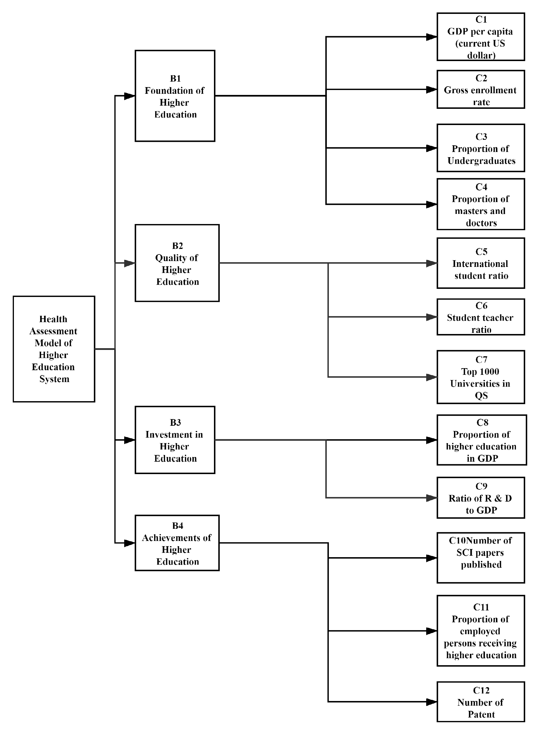
3.1. Design of Evaluation System

The first step is to choose indicators which summarize a national higher education system. In the process of indicator selection, we investigate a large number of educational evaluations at home and abroad, with reference to the indicator system and the content of national undergraduate teaching evaluation, as well.

According to the context, input, process, product (CIPP) model proposed by Yong et al. [22], we summarize the main contents of the development level of higher education as follows:

• Population, social and economic background of higher education: To understand the structure, process and achievements of higher education and various relationships between them, we first need to examine the basic conditions on which national higher education system relies. These conditions mainly include the situation of the population and social and economic development because these conditions restrict and affect the formulation and implementation of relevant higher education policies and affect the supply and demand of colleges and universities, teachers, teaching facilities and other higher education resources.
• Financial and human resources invested in higher education: These kinds of indicators mainly investigate the proportion of higher education institutions in national resources, the source of funds and the level of higher education used, as well as the number and proportion of all personnel employed in higher education departments. At the same time, these indicators also examine how financial funds for higher education are transformed to help students in their studies and scientific research.
• Access to higher education, participation and further study: Such indicators mainly include: (1) the participation rate of senior secondary education; (2) the participation rate of higher education (including public and private universities); (3) the participation in adult education; (4) the ratio of foreign students receiving higher education in China and Chinese students receiving higher education in foreign countries (the difference between exit and entry); (5) the type and proportion of adult workers participating in continuing education and training; (6) the dropout rate of private college students; and so on. The reason for adding the indicator is that international student mobility involves the economic expenditures and incomes of sending and receiving countries, as well as the corresponding brain drain.
• Social output and scientific output: These kinds of indicators mainly investigate the labor market output of higher education to the whole working age population, as well as the achievements of higher education in scientific research. These are: (1) the unemployment rate of students in higher education at all levels; (2) the proportion of employees receiving higher education; (3) the number of papers published; and (4) the number of patents published.

Based on the above research, we take the following four first-level indicators to describe higher education evaluation: higher education foundation, higher education investment, higher education process and higher education achievement. For the indicators that cannot be directly quantified, we use the secondary indicators represented by data to describe them more accurately. Referring to the two-stage semiparametric data envelopment analysis (DEA) model proposed by Wolszczak-Derlacz [23], we finally establish 12 second-level indicators. The framework of the evaluation model is shown in Figure 1.

3.2. Datasets and Methodology

In order to obtain the corresponding data of the selected indicator, we choose the following datasets: education at a glance, OECD indicators, world development indicators, world education report, web of science, China statistical yearbook. We select 8 representative countries (the United States, China, the United Kingdom, France, Australia, Egypt, Colombia and Vietnam) for data collection. These countries cover different levels of development and education. Each has its own focus on development of higher education. When selecting secondary indicators to evaluate the quality of higher education, we refer to the evaluation index system of QS World University ranking as shown in

Table 1. Evaluation indicator system of QS World University Ranking.

Standard	Second-Level Indicators	Weight
Research	Academic Reputation	40%
	Citations per faculty	20%
Teaching	Faculty/Student Ratio	20%
Employment Ability of the Graduate	Global Employer Reputation	10%
Internationalization	International Faculty Ratio	5%
	International Student Ratio	5%

.

At the same time, we encounter some obstacles. The evaluation system of QS ranking is comprehensive indeed, and its authority has been recognized all over the world. However, the latest QS ranking only includes 1300 universities in the world. These universities can represent the top level of higher education in the world, but they cannot reflect the development status of some ordinary universities and colleges in higher education. Taking China as an example, according to the 2020 national statistical bulletin on the development of education issued by the Ministry of Education, there are 2738 ordinary colleges and universities in China, with a total number of 41.83 million people in all kinds of higher education. However, 93 Chinese universities are included in the latest QS ranking, accounting for only 3.4% of the number of Chinese universities. It can be seen that if we evaluate the average level of higher education in a country as a whole, we need to choose some indicators that can not only reflect the average level of higher education but also reflect the differences between top universities and other universities. In the national statistical bulletin on education development in 2020, we note that the teacher-student ratio of undergraduate colleges is 17.51:1 and that of junior colleges is 20.28:1. It can be seen that there are relatively few teacher resources in junior colleges. In addition, in the 2019–2020 undergraduate teaching quality report, we observed that there is also a big gap in the study abroad rate of colleges and universities at different levels. Finally, we choose the proportion of teachers and students, the rate of studying abroad and the number of colleges and universities in QS ranking as secondary indicators to evaluate the quality of higher education. The repeated use of indicators may increase the complexity of the model and lead to over-fitting of the model. However, if we only evaluate the quality of national higher education according to QS ranking, the accuracy of the model will be reduced. Considering that our model only contains higher-education-related data in recent decades and the amount of data is small, we think it is acceptable to slightly increase the complexity to improve the accuracy.

3.3. Analytic Hierarchy Process (AHP)

AHP [24] is a simple, flexible and practical multicriteria decision-making method for quantitative analysis of qualitative problems. Combining quantitative analysis with qualitative analysis, this method applies decision-making rules to ascertain relative importance of achievable standards between measurement goals, with a reasonable weight for each standard of each decision plan. Weights are used to determine orders of pros and cons of each plan and more effectively applied to the problems that are difficult to solve with quantitative methods. The principles of AHP are briefly described in Algorithm 1.

Algorithm 1 Process of the AHP.

Input: Relative importance of each indicator

Output: Weighted matrix of evaluation system

1: Analyzing relationships among the various indicators and establishing a hierarchical structure of the system.

2: Comparing importance of same-level indicators pair-wise for a judgment matrix.

3: Calculating weights of each indicator by the judgment matrix.

4: Calculating general weights of the indicators in each level and sorting them.

3.3.1. Establishment of the Judgment Matrix

Analytic hierarchy process takes people’s judgment on the relative importance of each factor at each level as the information basis. These judgments are expressed by value and written in matrix form, which is called judgment matrix.

In the judgment matrix shown in

Table 2. The format of judgment matrix.

A	${\mathit{B}}_1$	${\mathit{B}}_2$	⋯	${\mathit{B}}_{\mathit{n}}$
$B_1$	$B_{11}$	$B_{12}$	⋯	$B_{1n}$
$⋮$	$⋮$	$⋮$	⋯	$⋮$
$B_m$	$B_{m1}$	$B_{m2}$	⋯	$B_{mn}$

, the relative importance of the indicator $B_i$ and the indicator $B_j$ can be expressed by $B_{ij}$. According to the scale of AHP in

Table 3. The scale of AHP.

Ratio of ${\mathit{B}}_{\mathit{i}}$ to ${\mathit{B}}_{\mathit{j}}$	Quantized Value ${\mathit{B}}_{\mathit{ij}}$
Equally important	1
A little more important	3
More important	5
Strongly important	7
Extremely important	9
The middle value between two judgments	2, 4, 6, 8

, numbers from 1 to 9 are applied to represent relative importance of factors at each level.

Due to the lack of specific data support for relative importance of various indicators, we assign values to the judgment matrix according to information we have and understand. This method is relatively simple but also subjective. Given enough resources in the future, we plan to assign value to the judgment matrix by means of questionnaire survey.

The judgment matrix should satisfy Formula (1):

$$B_{ji}=1/B_{ij}>0,B_{ii}=1$$

(1)

3.3.2. Consistency Check

In order to evaluate influence of hierarchy ranking, consistency of the judgment matrix is tested. We use the random consistency ratio ($CR$) to evaluate it. If $CR<0.1$, it indicates that the judgment matrix has satisfactory consistence. The first step of obtaining $CR$ is to calculate consistency index ($CI$) as follows.

$$CI=\left({\lambda }_{max}-n\right)P(n-1)$$

(2)

In Formula (2), ${\lambda }_{max}$ represents the maximum characteristic root of judgment matrix and n is the order of the judgment matrix. Then, in order to measure the size of $CI$, the random consistency index ($RI$) is introduced in Formula (3).

$$RI=\frac{C{I}_1+C{I}_2+\cdots +C{I}_m}{m}$$

(3)

For a fixed order n, we randomly construct m paired judgment matrices $A_1,A_2,\dots ,A_m$, and the values $a_{ij}$ in the matrices are randomly selected from $1,2,\dots ,9$ and $1/2,1/3,\dots ,1/9$. Such judgment matrices are inconsistent. We make m large enough to calculate $C{I}_1,C{I}_2,\dots ,C{I}_m$ and the average value $RI$ of $CI$. The values of $RI$ corresponding to different orders n are shown in

Table 4. The values of $RI$.

n	1	2	3	4	5	6	7	8	9
$RI$	0	0	$0.58$	$0.90$	$1.12$	$1.24$	$1.32$	$1.41$	$1.45$

.

$CI$ and $RI$ are compared to obtain the test consistency ratio ($CR$), shown in Formula (4).

$$CR=CI/RI=\sum W_{ci}{\left(CI\right)}_i/\sum W_c\left(R{I}_i\right)$$

(4)

We only focus on the case $CR<0.1$. It represents that comparison judgment matrix satisfies consistency and ranking weights are acceptable.

3.3.3. Calculate the Weight of Each Indicator

After confirming that an evaluation system is of consistency, we adopt three methods (arithmetic average method, geometric average method and characteristic root average method) to calculate average values of weights. Final weights of each indicator are shown in

Table 5. Weights of all layers.

General Purpose	First-Level Indicators	Secondary Indicators
A Health assessment model of higher education system	B1 Foundation of higher education (0.3198)	C1 GDP per capita (current US dollar) (0.4852)
		C2 Gross enrollment rate (0.2968)
		C3 Proportion of undergraduates (0.1090)
		C4 Proportion of masters and doctors (0.1090)
	B2 Quality of higher education (0.3632)	C5 International student ratio (0.2922)
		C6 Student-teacher ratio (0.0925)
		C7 Top 1000 universities in QS (0.6163)
	B3 Investment in higher education (0.1788)	C8 Proportion of higher education in GDP (0.5000)
		C9 Ratio of R&D to GDP (0.5000)
	B4 Achievements of higher education (0.1382)	C10 Number of SCI papers published (0.5396)
		C11 Proportion of employed persons receiving higher education (0.2970)
		C12 Number of patents (0.1634)

.

3.4. Technique for Order Preference by Similarity to an Ideal Solution (TOPSIS)

According to the indicator data and the weight matrix, we adopt the weighted TOPSIS to evaluate national higher education system.

3.4.1. Principles of TOPSIS

TOPSIS [25] is a common and comprehensive evaluation method which takes advantage of information from original data, and its results can accurately reflect pros and cons of evaluation schemes. The basic process is shown in Algorithm 2.

Algorithm 2 Process of weighted TOPSIS.

Input: Original dataset $X=\left\{x_1,x_2\cdots ,x_n\right\}$

The weight of each indicator $W=\left\{w_1,w_2,\cdots ,w_m\right\}$

Output: The higher education level of each research object

1: Normalizing indicator nature in the original dataset.

2: Constructing the normalized matrix $F=\left\{f_1,f_2,\cdots ,f_n\right\}$.

3: for $F_i$, each column of F do

4:    The $i\text{-}\mathrm{th}$ dimension of the worst plan $F^{-}$← the maximum value of elements in $F_i$.

5:    The $i\text{-}\mathrm{th}$ dimension of the best plan $F^{-}$← the maximum value of elements in $F_i$.

6: end for

7: for $f_i\in F$ do

8:    Determining the best plan $f_i^{+}$.

9:    Determining the worst plan $f_i^{-}$.

10:    Calculating $C_i^{+}$: the closeness between $f_i$ and $f_i^{+}$.

11:    Calculating $C_i^{-}$: the closeness between $f_i$ and $f_i^{-}$.

12: end for

13: Calculating the relative closeness of each evaluation object $C_i^{*}$.

14: Sorting $C_i^{*}$ according to the size of value.

3.4.2. Calculation of Weighted TOPSIS Method

The detailed calculation process is as follows.

Assume that there are m research objects and n evaluation indicators (attributes) and the i-th evaluation value of the j-th evaluation indicator is $x_{ij}$. Then, we set up the initial data matrix X.

$$X=\left(\begin{array}{cccc}{x}_{11}& x_{12}& \cdots & x_{1n}\\ x_{21}& x_{22}& \cdots & x_{2n}\\ ⋮& ⋮& ⋮& ⋮\\ x_{m1}& x_{m2}& \cdots & x_{mn}\end{array}\right)$$

(5)

Considering that the dimension of each index may be different, the initial judgment matrix X is normalized, and then we have the standardization matrix V.

$$V=\left(\begin{array}{cccc}{v}_{11}& v_{12}& \cdots & v_{1n}\\ v_{21}& v_{22}& \cdots & v_{2n}\\ ⋮& ⋮& ⋮& ⋮\\ v_{m1}& v_{m2}& \cdots & v_{mn}\end{array}\right)$$

(6)

Then, we define W as the evaluation indicators’ weight matrix and construct the weighted judgment matrix F.

$$\begin{array}{cc}\hfill F=VW=& \left(\begin{array}{cccc}{v}_{11}& v_{12}& \cdots & v_{1n}\\ v_{21}& v_{22}& \cdots & v_{2n}\\ ⋮& ⋮& ⋮& ⋮\\ v_{m1}& v_{m2}& \cdots & v_{mn}\end{array}\right)\left(\begin{array}{cccc}{w}_{11}& & & \\ & w_{22}& & \\ & & \ddots & \\ & & & w_{mn}\end{array}\right)\hfill \\ \hfill =& \left(\begin{array}{cccc}{f}_{11}& f_{12}& \cdots & f_{1n}\\ f_{21}& f_{22}& \cdots & f_{2n}\\ ⋮& ⋮& ⋮& ⋮\\ f_{m1}& f_{m2}& \cdots & f_{mn}\end{array}\right)\hfill \end{array}$$

(7)

According to the weighted judgment matrix F, we determine the ideal best plan and the ideal worst plan.

The ideal best plan:

$$f_i^{+}=\left\{\begin{array}{cc}\underset{j}{max}\left(f_{ij}\right),\hfill & \mathrm{the}\mathrm{positive}\mathrm{indicators}\hfill \\ \underset{j}{min}\left(f_{ij}\right),\hfill & \mathrm{the}\mathrm{negative}\mathrm{indicators}\hfill \end{array}\right.$$

(8)

The ideal worst plan:

$$f_i^{-}=\left\{\begin{array}{cc}\underset{j}{min}\left(f_{ij}\right),\hfill & \mathrm{the}\mathrm{positive}\mathrm{indicators}\hfill \\ \underset{j}{max}\left(f_{ij}\right),\hfill & \mathrm{the}\mathrm{negative}\mathrm{indicators}\hfill \end{array}\right.$$

(9)

The Euclidean distance between a research object and an ideal plan is calculated as follows.

$$\begin{array}{c}{C}_i^{+}=\sqrt{{\sum }_{j=1}^m{\left(f_{ij}-f_i^{+}\right)}^2}\hfill \\ C_i^{-}=\sqrt{{\sum }_{j=1}^m{\left(f_{ij}-f_i^{-}\right)}^2}\hfill \end{array}$$

(10)

The relative closeness of each evaluation object is calculated as follows.

$$C_i^{*}=\frac{C_i^{-}}{C_i^{+}+C_i^{-}},i=1,2,\dots ,m$$

(11)

$0\le C_i^{*}\le 1$, the closer $C_i^{*}$ is to 1, the better the research object is.

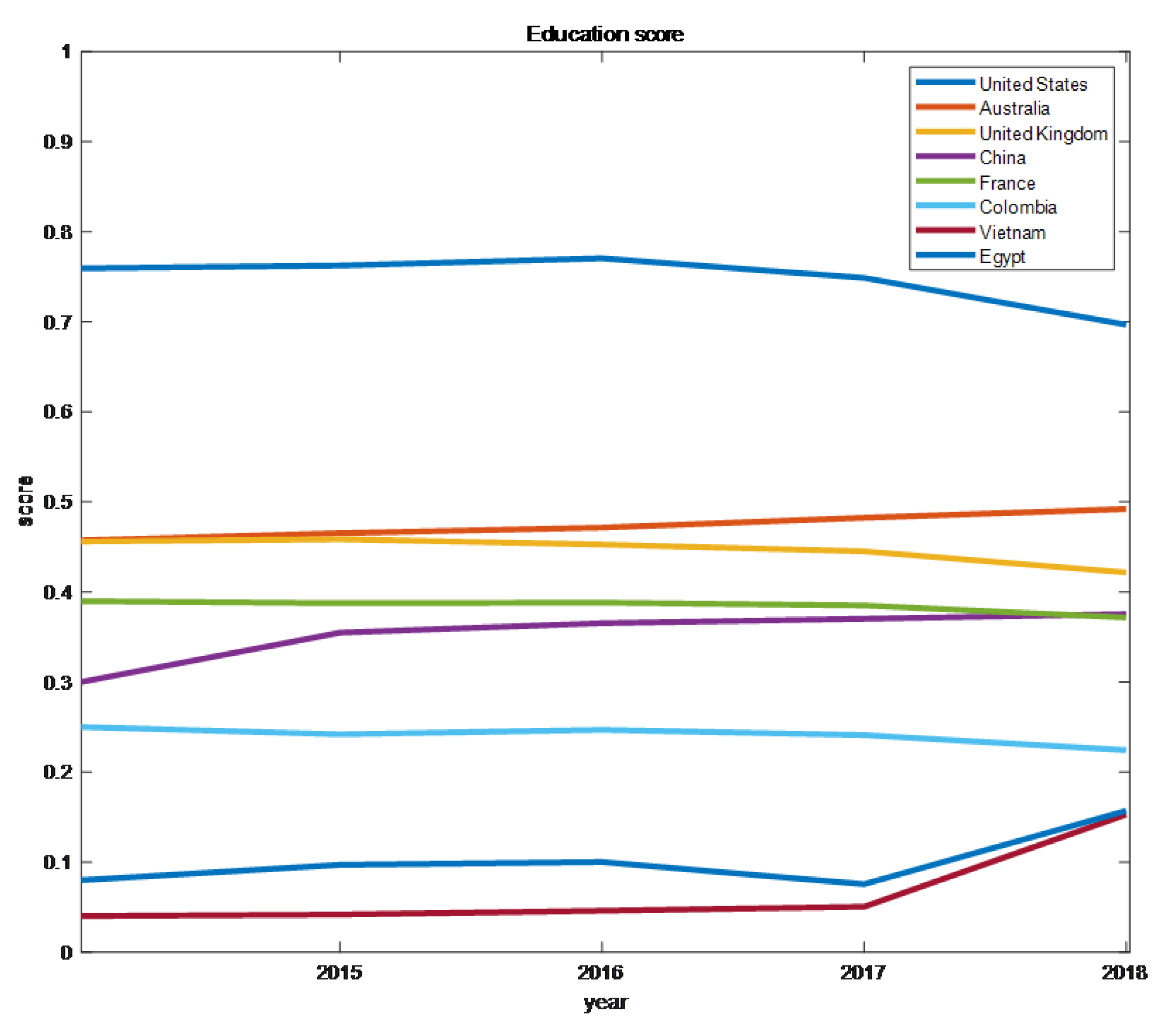
3.5. Evaluation of National Higher Education for Statistical Countries

Combining with the weight matrix obtained from AHP, we apply TOPSIS to the original data collected from the data source and calculate the quantitative evaluation scores of each research object from 2014 to 2018 as shown in Figure 2. In this way, the evaluation model is created based on both AHP and TOPSIS.

As shown in Figure 2, the higher education levels in developed countries are always in a leading position, while those in developing countries are relatively backward. Therefore, the evaluation results of this model present a good fit to reality. By analyzing the specific performance of each country, we find that the US has maintained the highest level over the whole five years. However, the evaluation score of the US presents a declining trend. In fact, due to the characteristics of TOPSIS reflecting relative levels, as time goes on, the gap between the US and any other country in the study presents a decreasing trend, as well. Furthermore, Britain, Australia and France are under the same level; the gap among them is very small. Moreover, Colombia’s level lies in the middle and has been relatively stable. The evaluation results of Egypt and Vietnam are not ideal, staying in the lowest level throughout the five years. However, in 2018, these two countries both presented obvious upward trends relative to the prior year. This indicates that countries with lower levels of higher education have considerable potential to develop. By examining Vietnam’s higher education policies [26], we realize that international cooperation provides opportunities for the development of higher education in a world of globalization and economic integration. Therefore, the Vietnamese government supports the expansion of international exchanges and encourages foreign capitals to invest in the research projects of the higher education system in Vietnam and beyond. The policies which the Vietnamese government adopt provide a valuable experience for the development of higher education in other countries.

In our model, China’s higher education has been significantly promoted. During just five years, China has developed from the same echelon as Colombia to the one close to some developed countries. In comparison with the US, which has the most advanced higher education system, there are still many areas for China to improve. In fact, data analyses show that the development of higher education in China is unbalanced, with some of the indicators remaining in a high level while others still staying low.

3.6. The State of China’s Higher Education Development

To better evaluate China’s higher education, we select the US as a reference because it claims the best education system worldwide. Focusing on 2018, as shown in Figure 3, we find that China falls behind the US in most indicators (the decrease in the student-teacher ratio represents the development of education levels to a certain extent), especially in the aspects of the proportion of undergraduates, the proportion of masters and doctors, the proportion of international students and the GDP per capita and educational investments, with an exception in the number of patents.

4. Higher Education Prediction Model

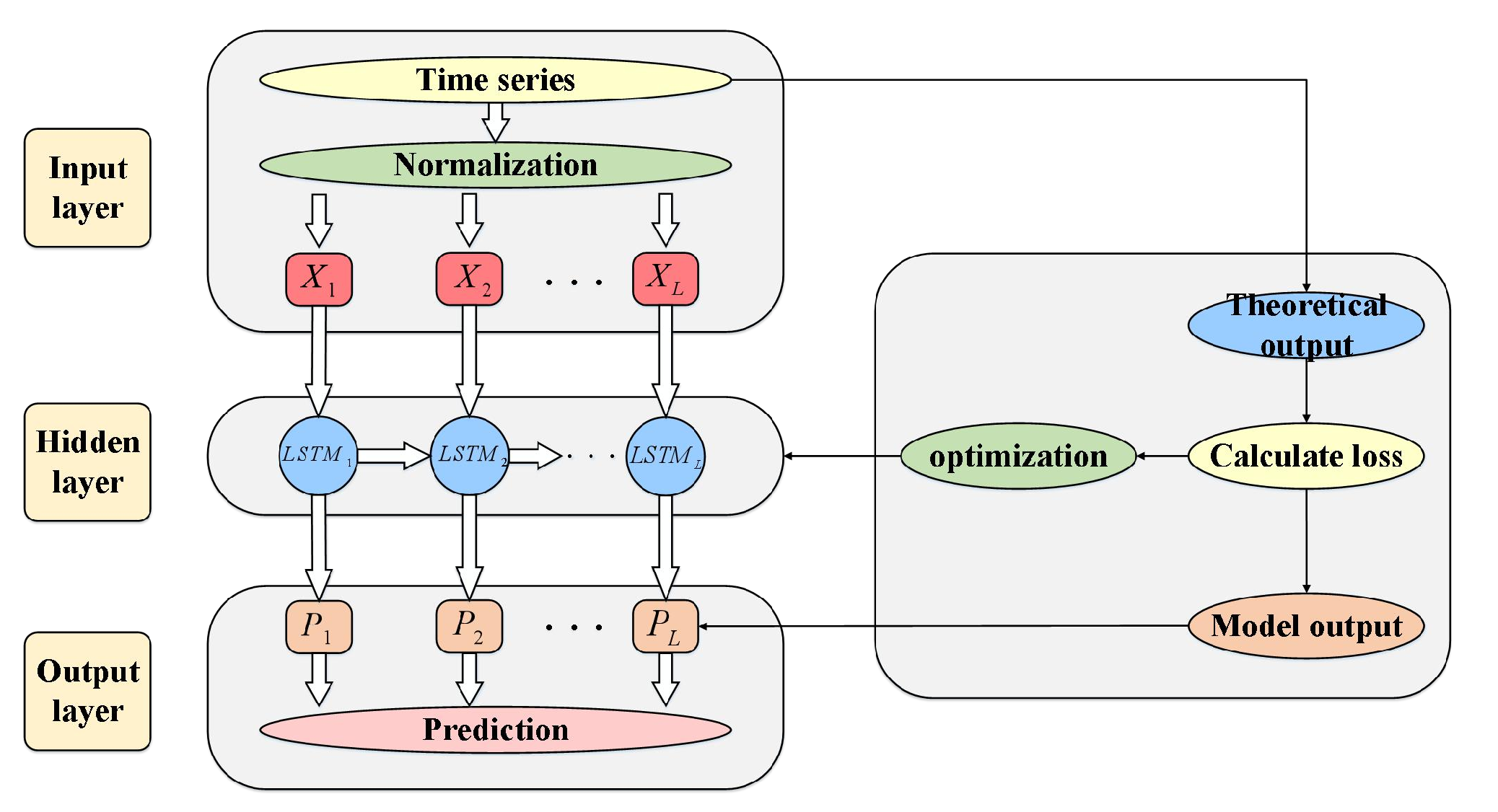
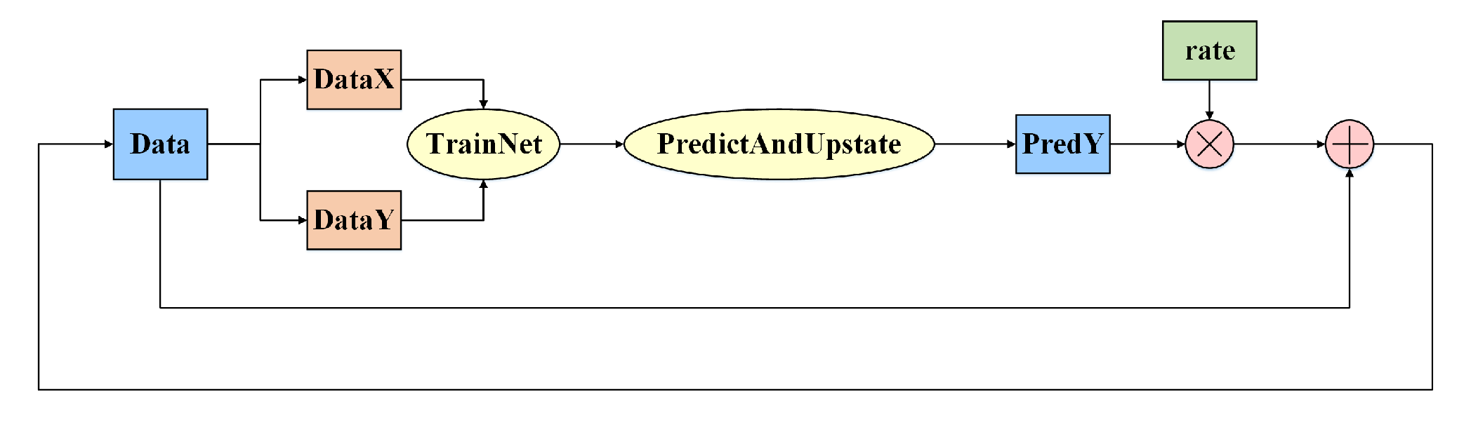
4.1. Framework of the Prediction Model

The overall framework of the prediction model in this paper is shown in Figure 4. The structure includes an input layer, a hidden layer and an output layer. The functions of the input layer include processing the original time series and normalizing the data to meet the requirements of the network input. The hidden layer is a single-layer cyclic neural network built by the LSTM memory unit. The output layer provides predicted results. In addition, the prediction model can optimize itself by calculating errors between model output and theoretical output.

4.2. Input Data of the Module

Considering data completeness, we select the data of various indicators in China from 2001 to 2018. Then, we apply the prediction model to the data in a time series.

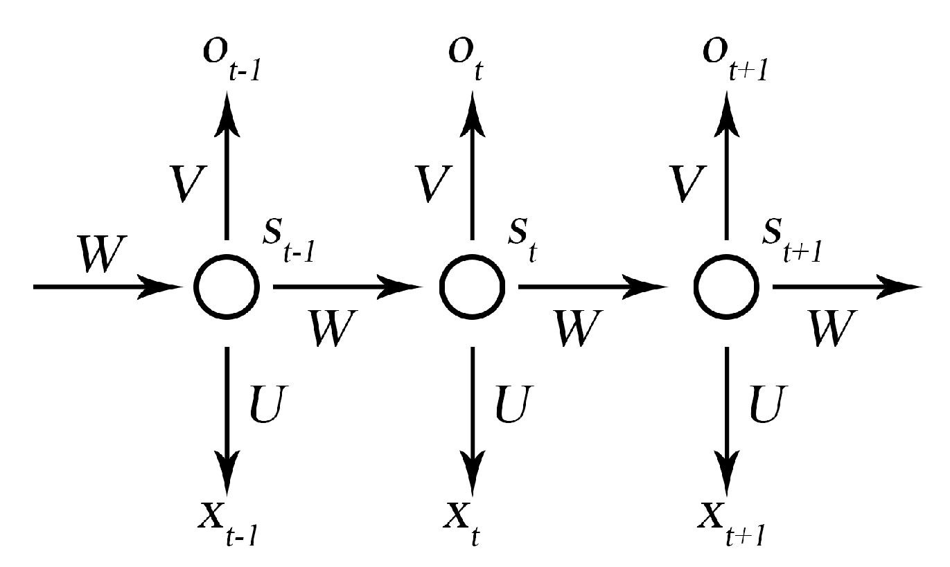
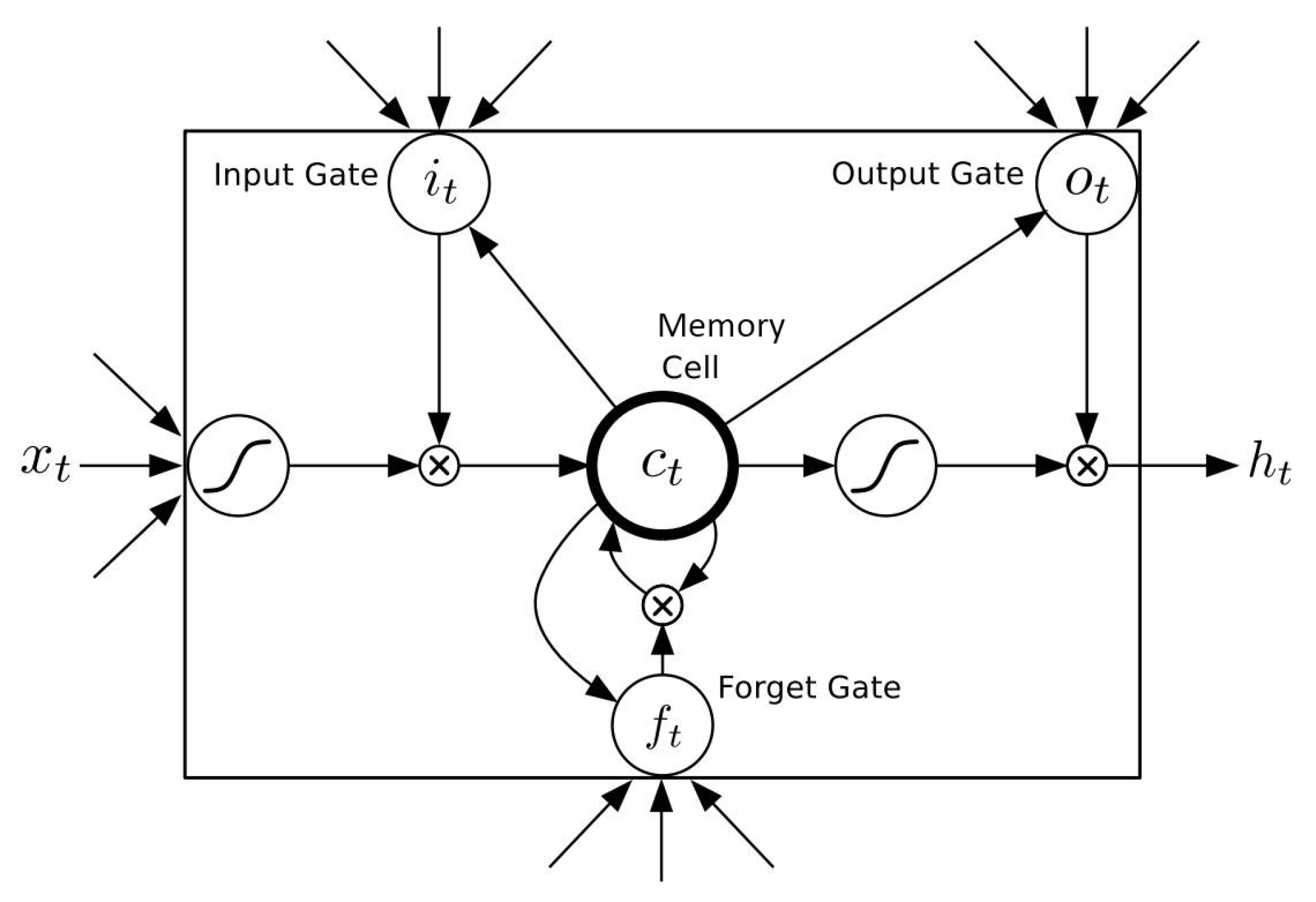
4.3. LSTM Neural Network

Long short-term memory (LSTM) is a special recurrent neural cetwork (RNN). It was introduced by Hochreiter [27] and Schmidhuber in 1997. As an excellent variant of RNN, LSTM inherits most of the characteristics of RNN models while addressing the vanishing gradient problem caused by gradual reduction in the gradient back propagation process. Specific to language processing tasks, LSTM is very suitable for dealing with problems that are highly related to time series, such as machine translation, dialogue generation, encoding and decoding. LSTM truly represents or simulates the cognitive processes of human behavior, logical development and neural organization. Since 2014, LSTM has become a very popular research model in RNNs and even deep learning frameworks.

All recurrent neural networks have the form of a chain of repeating modules of a neural network. In standard RNNs, this repeating module has a very simple structure, such as the repeating units in Figure 5.

Compared with RNNs, LSTM has a more complex structure, but its repeating modules have a different structure. Unlike a single neural network layer, there are four interacting parts in a very special way. The detailed structure of the current LSTM is shown in Figure 6.

All the units can make sigmoid nonlinear transformations, and input units can have arbitrary compression nonlinearity. The calculation of the whole LSTM network is described by Formulas (12)–(17):

$$i_t=\sigma \left(W^{i}H+b\right)$$

(12)

$$f_t=\sigma \left(W^{f}H+b^f\right)$$

(13)

$$o_t=\sigma \left(W^{k}H+b^k\right)$$

(14)

$$c_t=tanh\left(W^{c}H+b^c\right)$$

(15)

$$m_t=f_t\odot m_{t-1}+i_t\odot c_t$$

(16)

$$h_t=tanh\left(o_t\odot m_t\right)$$

(17)

In the formulas above, $i_t$ represents the input gate, $f_t$ represents the forgetting gate, $o_t$ represents output gate and $c_t$ represents memory cell. $\sigma$ is the sigmoid function, which is often used as the activation function of neural networks. $W^i$, $W^f$, $W^k$ and $W^c$ are the weight matrices. $b^i,b^f$, $b^o$ and $b^c$ are the corresponding offset terms. $m_t$ is the final state of memory cells and $h_t$ is the final output of the memory units. The hidden layer H consists of the new input vector $x_t$ and the previous hidden vector $h_{t-1}$ as shown in Formula (18).

$$H=\left(\begin{array}{c}{x}_t\hfill \\ h_{t-1}\hfill \end{array}\right)$$

(18)

4.4. The Segmentation Method of Time Series

We choose a previous series of length 1 to predict the time i. For a long enough time series (the length of the previous series used for prediction is much smaller than the total length of the time series), the basic algorithm is, according to the previous series’s length, established in Algorithm 3:

Algorithm 3 Algorithm of the time series data segmentation.

Input: Time series $T=\left\{t_1,t_2,\dots t_n\right\}$

Output: The aggregate of mapping relationships between previous series and target values $T^{\prime }=\left\{\left(X_1,Y_1\right),\left(X_2,Y_2\right),\dots ,\left(X_{n-l},Y_{n-l}\right)\right\}$

1: for $i=1:N$ do

2:    The previous series $X_{i-l}=\left\{t_{i-l},t_{i-l+1},\dots ,t_{i-1}\right\}$

3:    The corresponding value of the previous series $Y_{i-l}=\left\{t_i\right\}$

4: end for

5: Obtain the aggregate of previous series $X=\left\{X_1,X_2,\dots ,X_{n-l}\right\}$

6: Obtain the aggregate of target values $Y=\left\{Y_1,Y_2,\dots ,Y_{n-l}\right\}$

On Lines 1–4 of Algorithm 3, the index of time i is taken as the target value. According to the length of the previous series, we obtain the previous series used for prediction after segmentation. Then, in Lines 5–6, we obtain the previous series and target values of the dataset.

4.5. Circumstance Setting

The LSTM network needs to set up a reasonable circumstance according to applications in reality. Combined with the analysis of Vietnam’s higher education reform, we realize that the country’s macro control is essential to the development of higher education. Therefore, we decide to simulate a set of higher education policies and apply it to China in a predictive model to verify the feasibility of this set of policies and whether they can provide a reference for reality. In order to follow the principles of controlled experiments, we set up two circumstances, namely, one without policy and the other with policy.

4.5.1. Circumstance without Policy

Considering there is no policy intervention, the predictive results of various indicators in this environment only depend on the training effect of the LSTM network, and the training effect is directly determined by parameter setting. As such, for each parameter in LSTM, we set the number of hidden layers to 200, the loss function is defined by mean square error (MSE), the learning rate is set to 0.005 and the gradient threshold is set to 1. Then, we choose adaptive moment estimation (Adam), an optimization algorithm with learning rate adaption to optimize the model. Adam is considered to be robust to the choice of hyperparameters. According to the specific situation for different indicators to determine the appropriate number of training rounds, here we set the number of training rounds to 250. The whole values of parameters are shown in

Table 6. Set of Parameters.

Number of hidden layers	200
Loss function	MSE
Learning rate	0.005
Gradient threshold	1
Optimizer	Adam
Maximum training rounds	250

.

4.5.2. Circumstances with Policies

When considering circumstances with policies’ influence, we assume that the policies have a direct impact on various indicators of the evaluation model, and according to the pertinence of the policy, various indicators are affected in different degrees. On the one hand, if the main point of the policy is to develop the economy, then the indicators related to higher education investment will be significantly improved. Relatively speaking, the change in the teacher-student ratio may not be so noticeable. On the other hand, if the policy emphasizes enhancing international exchanges, the proportion of international students will also increase, while the impact on other indicators will be limited.

In general, a country’s higher education is closely related to its economic level, talent training mode and educational resources. At the same time, higher education is also the key driving force of national innovation, technological breakthroughs and industrial upgrading. In other words, the standard of higher education is closely related to the future of the country. At the same time, because higher education involves all aspects of society, the reform of higher education needs to started from multiple directions, which is a gradual process. Particularly for China, due to its population base, the opportunities provided by the current higher education system are relatively limited, resulting in violent involution. Thus, it is vital to innovate and create a higher education system and enrich educational resources.

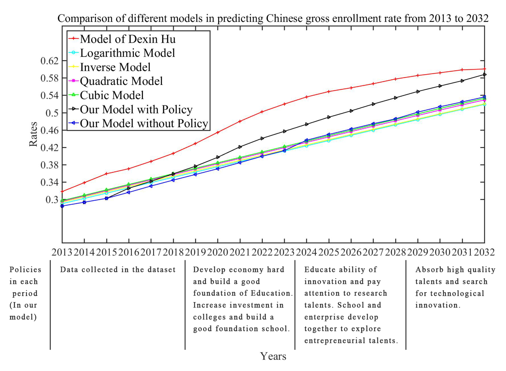
• Specific Policies and Timeline
  Considering that the national policies are not static, we assume that the policies are adjusted once every 5 years, and the current higher education system is evaluated periodically accordingly. While implementing the policies, we focus on the evaluation of China’s higher education. According to the model prediction results without policy influence, we design the policies and timeline as shown in

  Table 7. Policies and timeline.

  Time	2019–2023	2024–2028	2029–2033	2034–2038
  Important indicators	GDP per capita Gross enrollment rate Ratio of R&D to GDP Proportion of higher education in GDP	Proportion of undergraduates Proportion of masters and doctors International student ratio	Student teacher ratio Number of SCI papers Number of patents	International student ratio
  Corresponding policies	Develop hard economy and build a good foundation of education Increase investment in colleges and build a good foundation for schools	Educate the ability of innovation and pay attention to research talents School and enterprise developing together to explore entrepreneurial talents	Absorb high-quality talents and search for technological innovation	Broaden international horizon and improve the treatment of students

  . The timeline describes the key improvement indicators and corresponding policies every 5 years. Moreover, the timeline only represents the main implementation time, not the end time, of the policies.
  The details are illustrated as follows.

  –

  2019–2023: Build a good foundation

  (1) Strongly develop the economy and build a good foundation of education: According to the poverty line standard established by the world bank, as an upper-middle-income country, the number of poor people in China is calculated according to the standard of 5.50 international dollars per day. In the “World Bank East Asia and Pacific Economic Update—Spring 2022” [28] released on 4 April 2022, it is estimated that the total number of poor people in China in 2022 is 153 million, and the poverty rate comes to 10.83%. Although the number of poor people in China has decreased rapidly in recent years, it is undeniable that due to China’s huge population base, the poor population will still hinder China’s educational development. If we want to popularize higher education, we must strongly develop the economy and minimize the development differences between regions. Therefore, the first priority is to reduce poverty in poor areas and thus the proportion of the poor population while targeting the national economy for better GDP. In addition, it is important to improve basic education, particularly in those disadvantaged provinces. The more developed the basic education, the better the source of higher education for students.

  (2) Increase investment in universities and build a good foundation for schools: Universities are the foundation of higher education. Increasing investment in universities helps improve school environment and scientific research, which lead future universities to accommodate and train more outstanding talents and thus, in turn, build a good foundation for universities.

  –

  2023–2027: Innovation model

  (1) Educate the capabilities of innovation and emphasize research talents: China’s technological innovation has been a weakness, so universities should focus on training some research talents and improve students’ innovative capabilities. With the implementation of the policy from 2019 to 2023, the proportion of undergraduate students is expected to increase, as is the proportion of master’s and doctoral students through the cultivation of innovative research talents. Transforming undergraduates into high-quality and large-volume master’s and doctoral students is also a way to increase research talents to some degree.

  (2) School and enterprise developing together to explore entrepreneurial talents: Entrepreneurial talents are also necessary. We can innovate the school training system and cooperate with large enterprises, enhance the capabilities of innovation and entrepreneurship and promote the transformation of industrial innovation at the same time.

  –

  2028–2033: Key scientific research

  Absorb high-quality talents and search for technological innovation. At this stage, we need to focus on scientific research, introduce more excellent young scholars and teachers and reduce the ratio of students to teachers to ensure quality of teaching. By increasing investment in scientific research, we enhance the scientific research capabilities of colleges and research institutes and boost the output of papers and patents.

  –

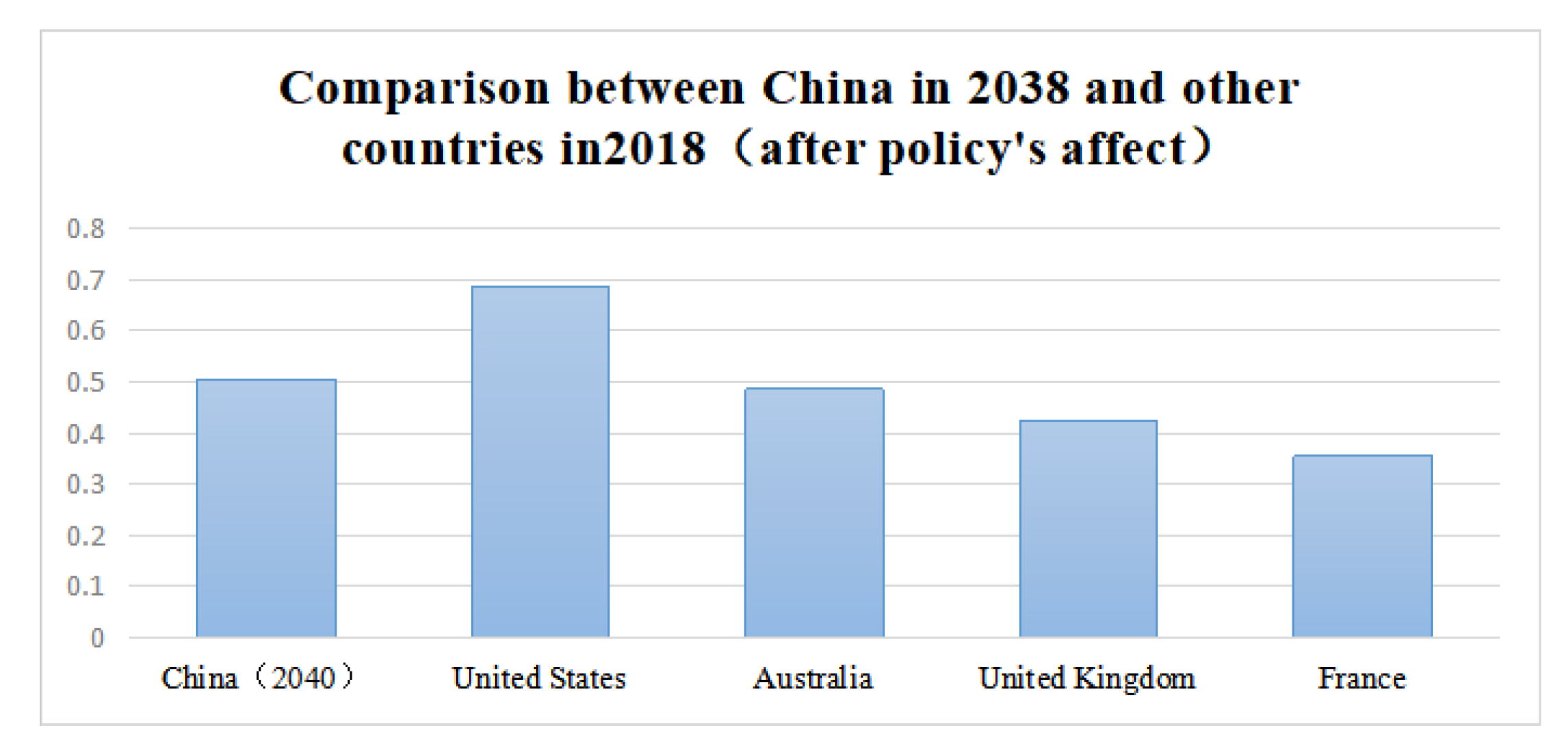
  2034–2038: Internationalization

  Broaden international horizon and improve treatment of international students. When the foundation of China’s higher education system develops, it becomes more attractive to top international talents and thus they are more inclined to study in China. If China further improves services for foreign students, the proportion of foreign students would rise even further, making the education system more open and diverse.

• Improvement of the Model After the policy’s formulation, we need to quantify the impact of the policy on all aspects of higher education and add it to the model. However, due to the lack of training set data, we refer to the econometric model of the impact of policy factors on China’s higher education investment proposed by Cheng et al. [29] and obtain constructive conclusions in this paper. In their paper, they made a quantitative analysis of the degree to which China’s education policy factors affected higher education investment from 1985 to 2007. The results of the model show that under the condition of determining the level of economic development, the impact of education policy on higher education investment is positive. However, under the limited conditions, such as the determination of the scale of college students, the impact of education policy on the total investment in higher education is negative. For instance, due to the impact of a series of major education policies promulgated and implemented in 1993, investment in higher education increased by an average of CNY 1 million under the condition that the economic aggregate remained unchanged and decreased by an average of CNY 40 million when the number of college students remained unchanged. In addition, after the enrollment expansion policy was implemented in 1999, the investment in higher education increased by an average of CNY 2 million under the condition that the economic aggregate remained unchanged, When the number of college students remains unchanged, the average decrease is CNY 5 million. Inspired by this paper, we define the impact of policies on different indicators. According to our model, when policies change, it impacts the prediction of the original series periodically. We assume the impact factor of policy on each indicator as $rate$. Obviously, $rate$ is sensitive to different indicators. In China, since the promulgation and implementation of policies generally take five years as a cycle, the $rate$ value of each cycle is the same. Combining with China’s specific national conditions, the values of $rate$ for each indicator in different cycles are shown in

  Table 8. The corresponding values of rate in different cycles.

  	2018–2023	2024–2028	2029–2033	2034–2038
  GDP per capita	0.6	0.5	0.3	0.3
  Gross enrollment rate	0.25	0.2	0.1	0.1
  Proportion of undergraduates	1	3	1	1
  Proportion of masters and doctors	4	6	3	3
  International student ratio	0.5	0.6	0.7	1
  Student-teacher ratio	−0.05	−0.05	−0.1	−0.05
  Ratio of R&D to GDP	0.2	0.2	0.1	0.1
  Proportion of higher education in GDP	0.3	0.3	0.2	0.2
  Number of SCI papers published	0.05	0.05	0.1	0.05
  Number of patents	0.02	0.02	0.05	0.02
  Proportion of employed persons receiving higher education	0.5	0.8	0.3	0.3

  .

Figure 7 shows the specific process of the optimized prediction model. We import the original data into the trained LSTM neural network to predict the time series in five years. Then, the result is multiplied by $rate$ and incorporated into the original sequence. Then, the new sequence is put into the model for the next round of prediction, and the final results are obtained through iteration. The calculation formula is as follows.

$$Net=TrianNet(XTrain,YTrain)$$

(19)

$$YPred=PredictAndUpstate(Net,YTrain)$$

(20)

$$Data=Data+YPred\times rate$$

(21)

In Formulas (19)–(21), $Net$ represents the LSTM neural network. $XTrain$ and $YTrain$ represent the data series. $TrainNet$ represents the function of training the LSTM neural network. $PredictAndUpstate$ represents the function of predicting and updating the LSTM neural network. $YPred$ represents the prediction result of the model. $Data$ represents the optimized output of the model. The value of $Data$ is renewed according to the product of $Ypred$ and $rate$.

5. Performance Evaluation

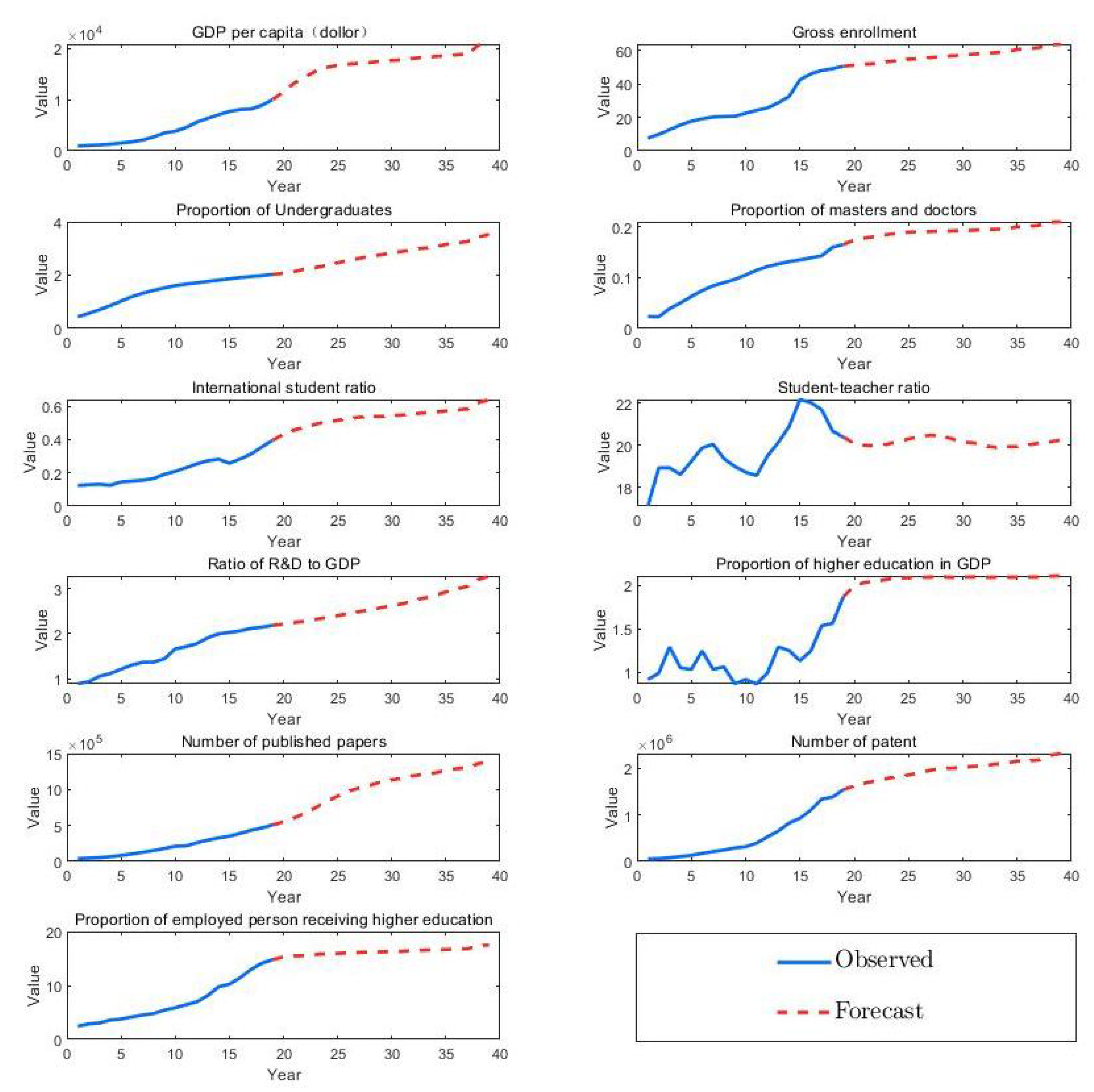
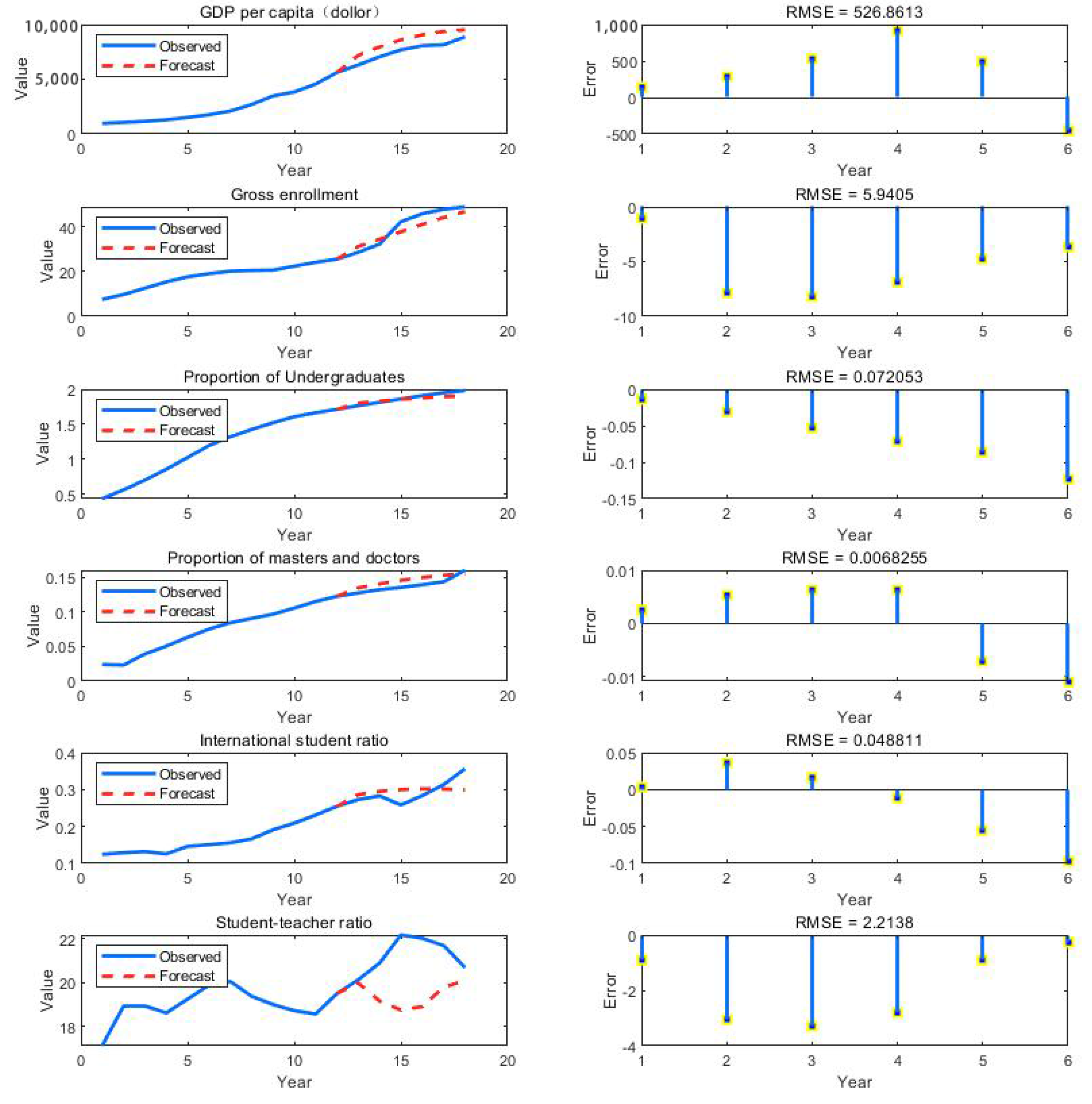
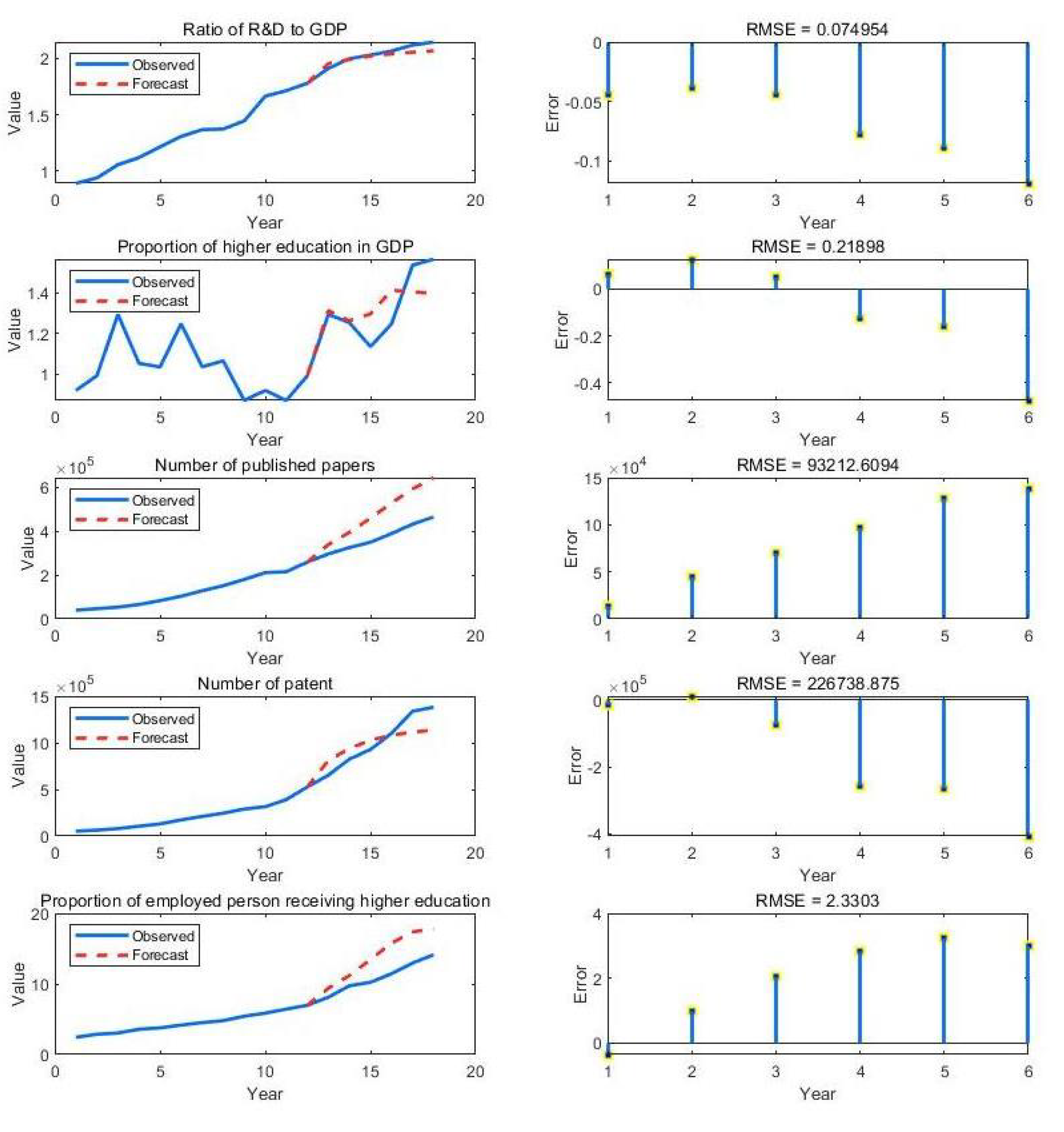
5.1. Experimental Results without Policy Influence

With all the preparations completed, we apply the original data to the LSTM network without policy influence. After iterative calculation, the predictive trends of China’s higher education indicators from 2019 to 2038 are obtained, as shown in Figure 8.

We import the prediction results of each indicator into the evaluation model to analyse the development of China’s higher education from 2019 to 2038, and then we compare the evaluation scores of China in 2038 with those of developed countries in 2018, and the results are shown in Figure 9.

If we do not adopt policies to the system, China’s higher education level in 2038 lies between Australia and the UK, but it still falls way behind the United States’, which is unsatisfactory. Thus, it is necessary to make corresponding policies to promote the development of the higher education system.

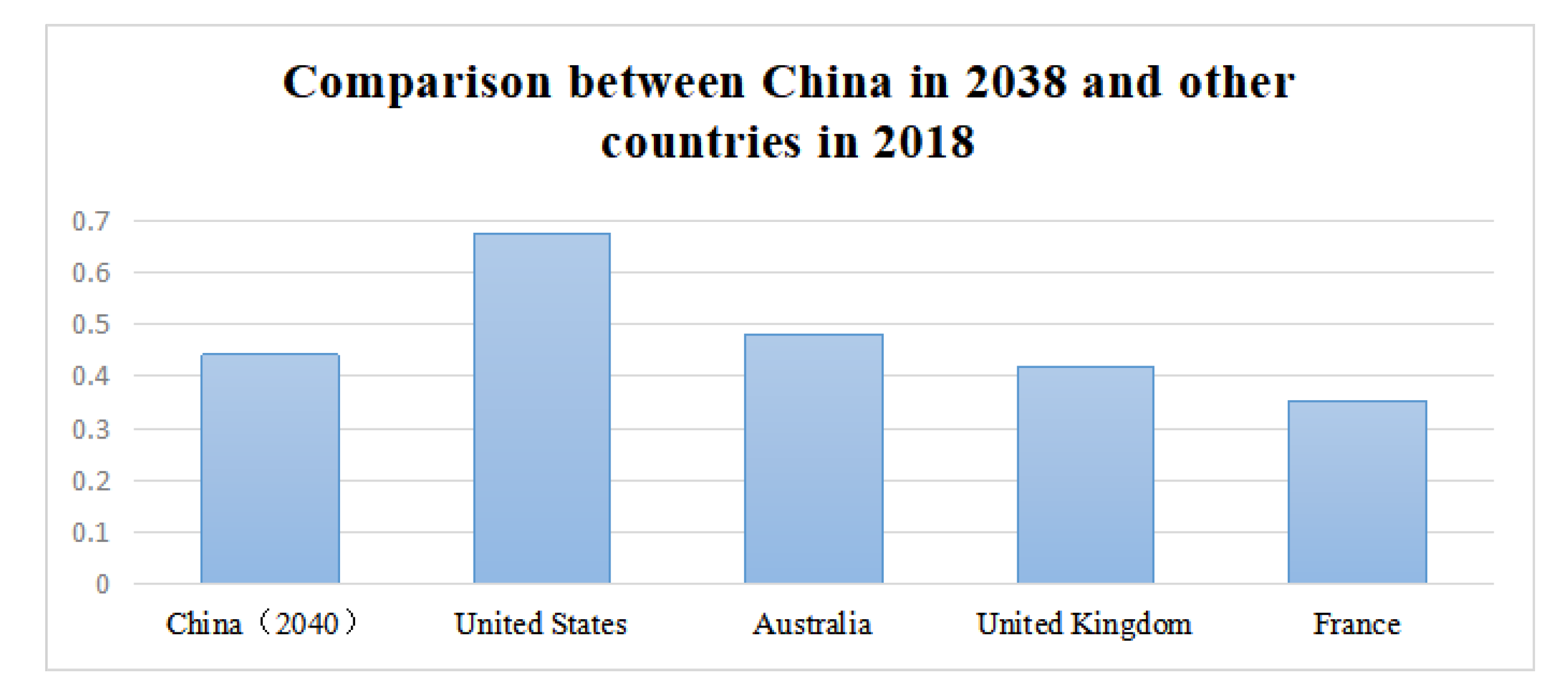
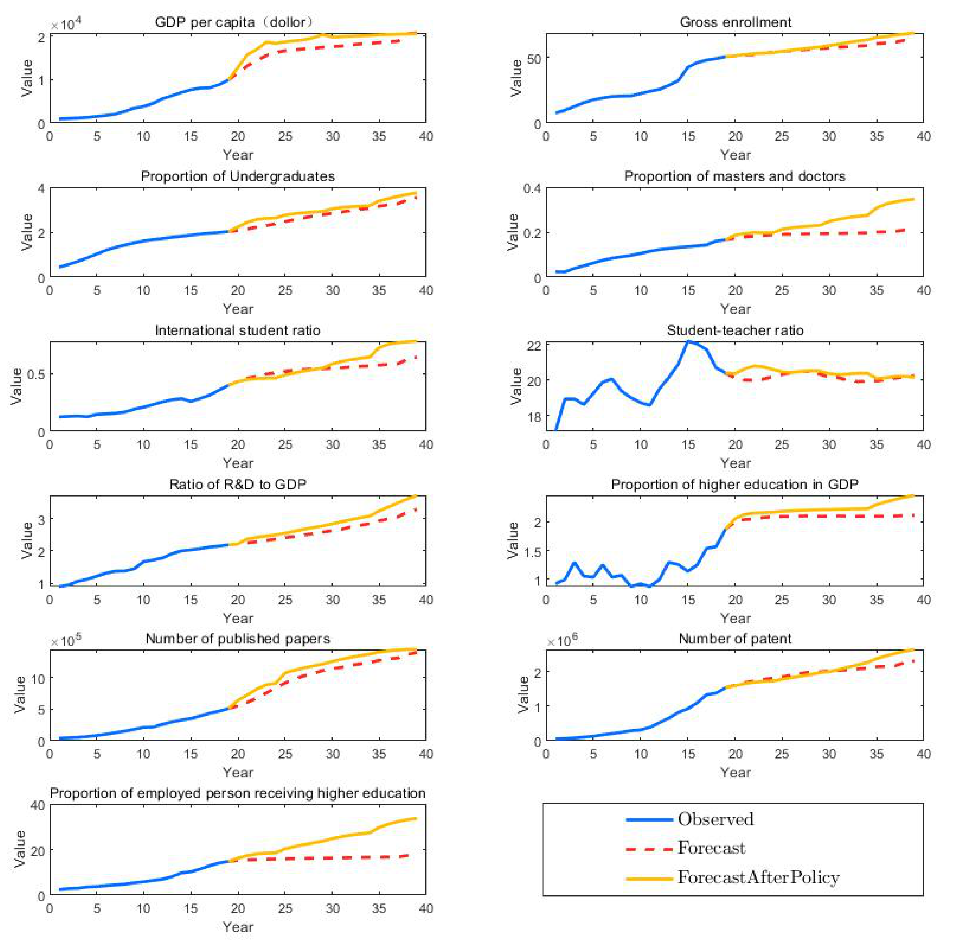
5.2. Experimental Results with Policy Influence

We apply source data to the improved LSTM network and then obtain experimental results shown in Figure 10. We find that under the influence of policies, the predicted values of each indicator exhibit different degrees of improvement relative to those without policy. Firstly, the proportion of masters and doctors and the proportion of employed persons receiving higher education are remarkably elevated by the policies, showing that our policies can significantly improve the popularization rate of higher education. However, economic indicators, including the proportion of higher education expenditures in GDP and the ratio of research and development (R&D) to GDP, present a small improvement. According to official data from the Ministry of Education of China, the proportion of national fiscal expenditures in education to GDP has remained above 4% for nine years (from 2013 to 2021). It can be seen that the predicted results are more in line with the actual trend. In addition, gross enrollment rate and teacher-student ratio are not apparently affected by the policies, indicating that the existing data for these two indicators have stabilized in our prediction model. However, in fact, gross enrollment rate and teacher-student ratio can reflect the richness of national higher education resources, so it is a significant sign of the development of higher education level. According to the experimental results, our policy adjustment seems to ignore this point, so we need to improve in this aspect. In addition, the indicators of scientific research achievements, including number of published papers and patents, show slight improvements. Existing policies can also be adjusted in this aspect. For example, the government can create and publish research journals on its own. However, note that the prediction results are not reasonable at times. For instance, the predicted international student ratio is apparently too high in comparison with the practical ones. According to the scale of the Chinese population, it is obviously unrealistic for the international student ratio to exceed 0.5. This problem brings up a challenge to the rationality of the prediction model. By examining the data of other research objects, we find that this abnormality is not uncommon. One of the possible explanations may be related to inaccurate data sources.

By adopting our evaluation model, we compare China’s performance with policy in 2038 with that of several developed countries without policy in 2018, and the results are shown in Figure 11. From the figure, we see that in 2038, China is expected to surpass the levels of higher education in the UK and France and reach the level of Australia in 2018. Certainly there is still a long way to go to catch up with the level of American higher education in 2018. However, in comparison with the situation without policy, the improvement is evident.

Impact of Policy Implementation

In the process of implementing the policies we have designed, students, teachers, universities, communities and country are all impacted. Details are discussed respectively as follows.

• For students: There will be gradually increasing opportunities for them to receive higher education, even with allowances for those poorer ones. However, rising gross enrollment rate and innovative requirements from the society lead universities’ students to compete more intensely. Their pressures from learning and competition remain after the policies are implemented, involving better study environments and more abundant teaching resources.
• For teachers: During the transformation period (SAME questions what to what), they will be better treated with more benefits and scientific research funds, which promote better research projects. Initially, the ratio of students to teachers increases, and so do the teachers’ duties. However, their burdens may be lessened after the implementation of new policies in 2029. With the implementation of supportive policies for scientific research and institutions, teachers’ capabilities required by the schools will be improved as well. These include teaching and scientific investigations, two main tasks for university teachers.
• For universities: It is valuable to raise construction funds, scientific research funds and the number and quality of students. However, this also brings pressure on the management of students, especially international students. At the same time, with continuous improvement in innovation and entrepreneurship training systems, universities need to keep a balance between enterprises and scientific research. It is a long-term goal for universities to be diversified and top-notch in teaching and scientific research. Such a transformation comes with great pressure. Even afterwards, universities need to constantly make adjustments to adapt to reality.
• For countries: As for reforms in the higher education system, the fundamental purpose is to make the system play a better role in promoting economic development and industrial innovation. There are going to be resistances and difficulties facing the national reforms. Constructions of basic education, the combination of schools and enterprises and investments in universities all have an impact country-wide. After the transformation, the higher education system will be gradually improved with national supports and therefore promote social progresses and national developments. However, in the process of transformation, there will be great resistance, such as the problem of funds, whether the results can be produced on time, the problem of multicultural interaction with the increase in foreign students and the problem of academic stress. According to our prediction, it is very difficult to improve the education system in the short term.

5.3. Sensitivity Analysis

To reflect the realities of prediction model errors and analyze the sensitivity of the model for subsequent optimization, we adopt a data prediction model with an optimization method based on root mean square error (RMSE), which is determined by the following formula:

$$RMSE=\sqrt{\frac{{\sum }_{i=1}^n{\left(p_i-a_i\right)}^2}{n}}$$

(22)

In Formula (22), $a_i$ represents the real data and $p_i$ represents the predicted data. We can find that RMSE is more sensitive to exceptional values. When there is a big difference between observed values and real ones, RMSE tends to be very large, so RMSE is used to verify the accuracy of network training.

The detailed optimization proceedings are as follows:

• Preprocessing: For variables to be predicted in the dataset, we calculate their periodic values and rank them from small to large. Next, we obtain the periodic values of the first N smallest variables to be predicted. Then, we calculate the correlation coefficients between the variables and those to be predicted and arrange the variables in order from large to small according to their corresponding correlation coefficients. Finally, we extract the variables with sums of correlation coefficients being greater than a coefficient threshold to form a training set.
• LSTM modeling: We organize the training set into a time sequence and input the time sequence into the LSTM network composed of multiple connected LSTM units to obtain the current training model.
• Optimizing: We use the training model to calculate the values of the variables predicted at the set time and compare them with the actual values of the variables predicted to obtain the root mean square errors (RMSEs). Compared with the RMSEs of previous rounds of training, the smaller values are taken as the RMSEs of current rounds of training, and the corresponding training model is reserved as the optimal solution model.

In the training of the LSTM neural network, we divide the dataset into the training dataset and the test dataset according to the ratio of 2:1. Then, we input the test dataset into the trained neural network to output the prediction dataset, and we calculate the RMSE values. The results are illustrated in Figure 12. We see that the predicted values of most indicators in our model are highly consistent with the observed ones, although the predicted curves of some indexes are quite different from the observed ones. For example, the predicted values of the student-teacher ratio are lower than the observed, and the predicted values of the proportions of higher education in GDP decrease and then rise sharply in the observed curve. In addition, the predicted values of the number of published papers and the proportions of employed persons receiving higher education are both obviously higher than their observed.

Due to the small size of available data, the predictions of some indicators are not ideal, but overall trends are much more consistent with the true values, with errors within an acceptable range. If we increase the size of the original data, consistency becomes even better. Furthermore, it appears from Figure 12 that the RMSE of each indicator is relatively small, and it shows that the predicted values are close to their real ones, which verifies the rationality and robustness of the model.

5.4. Comparison with Other Models

In order to further determine the accuracy and complexity of the model, we compare the predicted results with those from existing models. In order to do so, we need to define the criteria when comparing different models.

The criteria for determining the quality of a model mainly refer to two indicators: one is accuracy, and the other is complexity. They are usually contradictory. An increasing number of variables improves model accuracy but leads to a more complex model which may be in danger of over-fitting. Furthermore, less accurate models may be incapable of an adequate description of the dataset. Therefore, we attempt to find a balance between accuracy and complexity, usually with accuracy first and complexity second.

From the previous investigations of existing models, we note that those studies mainly focus on a single indicator of a large higher education system, such as financial investment scale [30], population growth [31] or higher education popularization [32]. Their research methods are also one-dimensional, such as the auto-regressive integrated moving average (ARIMA) model [33] or regression model. In comparison with our comprehensive model, these existing models yield less accurate results but reduce computational complexity without considerations of multiple factors.

To further illustrate accuracy and complexity, we choose China as an example again. When selecting the indicators for comparison, the existing models often use gross enrollment rate as an evaluation indicator. We determine that two models with close prediction ranges and indicators are better to be compared.

In this section, our LSTM prediction model is compared with existing models, such as the rolling regression models proposed by Li et al. [34] and the logarithmic prediction model proposed by Hu et al. [35]. Based on the statistics of higher education scale over the years, Li et al. [34] constructed a variety of fitting models to simultaneously predict and compare the results of various methods to reduce random errors in method selection. Finally, by comparing the coefficient of determination $R^2$ of different prediction models, four rolling regression models (logarithmic, inverse, quadric and cubic) with relatively high $R^2$ values are applied to predict the gross enrollment rate from 2013 to 2030.

In the case of the logarithmic prediction model, Hu et al. [35] proposed a model based on economic level to predict the gross enrollment rate and number of students in higher education from 2016 to 2032. They also used various regression models to reduce errors and more accurately predict the development of higher education. Combined with the judgment coefficient R2 and F value, the logarithmic model has the best-fitting degree; the prediction results are relatively close to the real data. Therefore, the logarithmic curve is finally chosen as the model for predicting the development of higher education. Combined with the prediction time range of each model, in order to ensure that the data of each model are fully utilized, we select the data from 2013 to 2032 for comparison. Then, we replace the missing data from 2013 to 2018 in our model with real data.

The comparison between the predicted results of the existing model and those of our designed model is shown in Figure 13. Seen from Figure 13, the gross enrollment rates predicted by all models are apparently in rising trends. The predicted values of the four regression models designed by Li et al. [34] present little differences, which represent the standard deviations from the concentrated trend, but the average index tends to be the same. In addition, the average annual growth rates of the gross enrollment rates obtained by the models are also very similar. In addition, the predicted values of each model can be verified with one another, which shows that the results obtained by the time series method are consistent. However, the slopes of the four models tend to be constant, indicating that the prediction results tend to be homogeneous and idealized if only relying on the regression equation to fit the predictive line and ignoring the influences of practical factors.

In addition, the predicted results of the model of Hu et al. [35] are significantly higher than those of other models, considering that the initial value of the model is higher than that of other models. The reason may be that the data source is different from the other ones. At the same time, the slope of the curve of the model has a more evident change, and the growth rate gradually slows down in a later stage. Considering the complicity in reality with multiple factors, it is more reasonable to recognize that the growth rates fluctuate to a certain extent rather than being constant.

Our predicted values without policy are quite close to the predicted values of the four models proposed by Li [34]. This reflects that the predicted results of our model are more idealized when there is no policy intervention. However, the predicted curves of our model with policy are unique in all curves. It appears that the curve starts from the lowest initial value and ends with the second highest predicted value in 2032. Moreover, the change in slope represents the influences of corresponding policies. From 2019, when the policies, which can improve the gross enrollment rate, are implemented, the slope increases significantly. Our model can not only predict the development trend of gross enrollment ratio in an idealized environment but also takes into account practical factors. Additionally, it can also have corresponding feedback for different policies, so it has a greater reference value for reality.

After the accuracy is verified, we compare the complexity. The complexity of the model can be described by many indicators and has a certain subjectivity. In machine learning, model complexity usually refers to the number of features or terms contained in a given prediction model and whether the selected model is linear or nonlinear. It can also refer to algorithm learning complexity or computational complexity.

There is a risk of over-fitting for a model with much complexity, and it may be more expensive in calculation, as is the case with LSTM. For example, Google translation only applies the LSTM network structure of seven to eight layers.

The calculation complexity of each update of LSTM is:

$$O(KH+KCS+HI+CSI)=O\left(W\right)$$

(23)

$$W=KH+KCS+CSI+2CI+HI=O(KH+KCS+CSI+HI)$$

(24)

In the formula above, K represents the number of output units. C represents the number of memory units. S (S > 0) represents the size of memory units. H is the number of hidden units. I is the number of units directly connected with memory units, gate units and hidden units, and W is the number of weights.

The complexity of the four rolling regression models designed by Li et al. [34] and the logarithmic prediction model proposed by Hu et al. [35] is O($y^3$) or less, and y represents the data of the training dataset. Thus, the model complexity of single-update LSTM is higher than that of other models, which leads to the disadvantage of LSTM in computing speed and depth calculation. However, due to the relatively small data range selected by our model, the risk of calculation-related, time-consuming and gradient problems is limited in our model.

5.5. Some Defects of Our Model

We try our best to ensure the comprehensiveness of the indicators, but some more complex factors are omitted, such as age structure of a country, youth population and influence of various extreme conditions. These factors are likely to have a great impact on a country’s higher education system, which is also where our model needs to be improved.

As a matter of fact, for two years, the worldwide COVID-19 epidemic has brought disruptive changes to higher education systems in many countries. For instance, at the beginning of the epidemic, China was severely impacted. At the same time, the Chinese government formulated strict epidemic prevention policies, such as blocking transportation in many large cities, limiting residents at home in the epidemic areas or even mandating individual isolation. Such measures effectively controlled the spread of the epidemic but obviously also had a great impact on all walks of life in China. In 2020, the growth rate of China’s GDP per capita was 2.2%, the lowest in recent years. Some industries have been greatly impacted by the epidemic, while others have had better developmental opportunities. In addition, it is difficult for students to learn efficiently and cultivate and enhance their skills greatly when limited indoors. Further, the epidemic leads to many international travel limitations and thus less opportunities for them to study abroad. In some countries, even the demographics and number of school-age populations are changed due to severe epidemics. These all have implications for the evaluation of higher education.

Additionally, we ignore interactions between certain indicators in the model. For example, an increase in unemployment may lead to an increase in the gross enrollment ratio, as laid-off workers seek to improve their future employment prospects to continue their studies. On the one hand, politically stable and economically prosperous countries may also bring many beneficial factors to the development of higher education, such as higher investment in education and more output of scientific research, and the attraction to overseas talents may also be enhanced. On the other hand, scientific research also has a positive effect on national development. Some of the research results in papers and patents are applied in practice and provide convenience for production and living. It will effectively help improve the country’s economy and, in turn, provide more expenditures in education and scientific research.

6. Conclusions and Future Work

In this paper, we establish a higher education evaluation model based on AHP, TOPSIS and LSTM. With this model, we are able to evaluate the higher education system and predict future developments of the system in most countries.

The experimental results indicate that the higher education evaluation of our model in various countries is consistent with reality, which is generally high in developed countries and low in developing countries. Additionally, our prediction results are also more in line with the actual data than that of other existing models, while a few exceptions exist, such as the prediction of the number of academic papers published. In summary, our model basically achieves the goal of universal applicability and accuracy.

According to the results of the model, the following are suggested for a government’s education policy:

• Standardizing investment behavior. While encouraging the expansion of the investment scale of higher education and scientific research, we should also avoid the waste of social resources caused by ineffective investment. The waste of resources is mainly concentrated in the aspects of material and financial. On the one hand, currently, many colleges and universities have the phenomenon that the utilization rate of scientific research equipment is low or even idle. According to the statistics of the State Education Commission of the PRC, more than 20% of instruments and equipment in universities across the country are idle, and the utilization rate of expensive large-scale scientific research equipment is no more than 15%. On the other hand, a few researchers apply for scientific research projects purely for “money”. Once the scientific research project is established, they ignore the rationality and efficiency of the use of funds, resulting in the false use of project funds and serious economic waste. Thus, achieving a rational allocation of resources and making the best use of educational investment is of great significance for accelerating the development of higher education.
  In view of the above waste of resources, we can make the following suggestions: In the aspects of resource investment, the government should reduce direct investment and encourage universities to seek funding channels by improving education quality and efficiency. In the management of universities, we should improve the use efficiency of teaching instruments and equipment, avoid the waste caused by the repeated purchase of equipment as far as possible, standardize the use of instruments by teachers and students, reduce the cost of maintenance and the loss of instruments and equipment and make the best use of ground objects to the greatest extent. Be familiar with the macro development trend of higher education and create a development environment that conforms to the trend of the times for higher education. Higher education is always influenced by the macro trends taking place in the surrounding world, which will shape the future of higher education and teaching. For example, due to the implementation of some university construction projects, the international ranking of Chinese universities has been rising rapidly. On the other hand, it has also caused a serious uneven distribution of resources among universities. The economically developed eastern region of China occupies a vast amount of educational resources. Even if some universities in the western region have a deep foundation, they are gradually overtaken by the eastern universities due to a lack of resources. In addition, teachers’ degrees in China’s colleges and universities have generally improved, which also makes the competition for teachers’ positions increasingly fierce, and the student-teacher ratio has increased slightly. In addition, the digital learning environment is changing the way higher education institutions build learning ecosystems for learners and teachers. Higher education institutions increasingly need to support open standards in the application of educational technology so that they can provide more students with a flexible learning experience. The current situation and development trend of higher education will provide a general direction for the government’s policy making.
  After understanding the development status of China’s higher education, we can put forward the following suggestions: (1) Advocate the effective exchange of regional educational resources, such as the mode of the joint running of colleges and universities and the mutual recognition of course examination results established in Wuhan. Thus, we can further integrate regional educational resources. (2) Give full play to the role of open education resources to promote the sustainable development of online education. (3) Pay attention to the individual differences among students and realize the accurate allocation of teaching resources according to the different learning conditions of students. Carry out reforms of the talent training system, including the integration of interdisciplinary scientific research and teaching. Higher education institutions can be encouraged to carry out wide-area interdisciplinary scientific research on major social issues, such as water cleaning, environmental sustainable development, gender equality, high-risk language protection and local noncultural heritage protection. In addition, the establishment of national laboratories, online periodical resource platforms and interschool collaborative network platforms promote necessary infrastructures and resources for high-quality graduate education.

While emphasizing these applications and suggestions above, we recognize some problems in the model.

Thus, more work needs to be conducted to better our model and further address the issues. Technically, more indicators are to be enriched to improve the complexity of the model, and calculation optimization needs extra examination. Further, it is recognized that building a healthy and sustainable higher education system is never an easy target. With globalization, policy adjustments and higher education reforms face more complexities and difficulties. Innovative ways of teaching from artificial intelligence, which has been greatly developed lately, also have an impact on educational qualities and success. These factors need to be considered as well in the future.

References

- Millot, B. International rankings: Universities vs. higher education systems. Int. J. Educ. Dev. 2015, 40, 156–165. [Google Scholar] [CrossRef]
- Yi, M.C. Popularization process of higher education in China and its influencing factors—Prediction based on time series trend extrapolation model. China High. Educ. Res. 2016, 3, 47–55. [Google Scholar]
- Pereira, C.A.; Araujo, J.F.; Maria, M.T. The Brazilian higher education evaluation model: “SINAES” sui generis? Int. J. Educ. Dev. 2018, 61, 5–15. [Google Scholar] [CrossRef] [Green Version]
- Khatibi, V.; Keramati, A.; Shirazi, F. Deployment of a business intelligence model to evaluate Iranian national higher education. Soc. Sci. Humanit. Open 2020, 2, 100056. [Google Scholar] [CrossRef]
- Benito, M.; Gil, P.; Romera, R. Evaluating the influence of country characteristics on the Higher Education System Rankings’ progress. J. Inf. 2020, 14, 101051. [Google Scholar] [CrossRef]
- Kajol, R.S.; Neethu, K.P.; Madhurekaa, K.; Harita, A.; Mohan, P. Parallel SVM model for forest fire prediction. Soft Comput. Lett. 2021, 3, 100014. [Google Scholar]
- Gao, Y.F.; Hang, Y.; Yang, M.L. A cooling load prediction method using improved CEEMDAN and Markov Chains correction. J. Build. Eng. 2021, 42, 103041. [Google Scholar] [CrossRef]
- Duan, H.M.; Pang, X.Y. A multivariate grey prediction model based on energy logistic equation and its application in energy prediction in China. Energy 2021, 229, 120716. [Google Scholar] [CrossRef]
- Arar, M.F.; Ayan, K. A feature dependent Naive Bayes approach and its application to the software defect prediction problem. Appl. Soft Comput. 2017, 59, 197–209. [Google Scholar] [CrossRef]
- Ekmekcioglu, O.; Koc, K.; Ozger, M. Stakeholder Perceptions in Flood Risk Assessment: A Hybrid Fuzzy AHP-TOPSIS Approach for Istanbul, Turkey. Int. J. Disaster Risk Reduct. 2021, 60, 102327. [Google Scholar] [CrossRef]
- Bakioglu, G.; Atahan, A.O. AHP integrated TOPSIS and VIKOR methods with Pythagorean fuzzy sets to prioritize risks in self-driving vehicles. Appl. Soft Comput. 2020, 99, 106948. [Google Scholar] [CrossRef]
- Azimifard, A.; Moosavirad, S.H.; Ariafar, S. Selecting sustainable supplier countries for Iran’s steel industry at three levels by using AHP and TOPSIS methods. Resour. Policy 2018, 57, 30–44. [Google Scholar] [CrossRef]
- Vasan, D.; Alazab, M.; Wassan, S.; Safaei, B.; Zheng, Q. Image-Based malware classification using ensemble of CNN architectures (IMCEC). Comput. Secur. 2020, 92, 101748. [Google Scholar] [CrossRef]
- Chen, W.L.; Yeo, C.K.; Lau, C.T.; Lee, B.S. Leveraging social media news to predict stock index movement using RNN-boost. Data Knowl. Eng. 2018, 118, 14–24. [Google Scholar] [CrossRef]
- Inoue, K.; Hara, S.; Abe, M.; Hojo, N.; Ijima, Y. Model architectures to extrapolate emotional expressions in DNN-based text-to-speech. Speech Commun. 2021, 126, 35–43. [Google Scholar] [CrossRef]
- Atila, O.; Sengur, A. Attention guided 3D CNN-LSTM model for accurate speech based emotion recognition. Appl. Acoust. 2021, 182, 108260. [Google Scholar] [CrossRef]
- Yan, Y.; Xing, H.Y. A sea clutter detection method based on LSTM error frequency domain conversion. Alex. Eng. J. 2021, 61, 883–891. [Google Scholar] [CrossRef]
- Zhang, J.; Li, K.K.; Wang, Z. Parallel-fusion LSTM with synchronous semantic and visual information for image captioning. J. Vis. Commun. Image Represent. 2021, 75, 103044. [Google Scholar] [CrossRef]
- Gao, X.; Li, W.D. A graph-based LSTM model for PM2.5 forecasting. Atmos. Pollut. Res. 2021, 12, 101150. [Google Scholar] [CrossRef]
- Zhao, X.; Rui, X.T.; Li, C.; Ma, Z.Z.; Miao, Y.F. Evaluation and prediction methods for launch safety of propellant charge based on support vector regression. Appl. Soft Comput. 2021, 109, 107527. [Google Scholar] [CrossRef]
- Huang, K.; Lu, S.L.; Yuan, J.; Han, Z.; Wang, C.; Zhoua, Z. Evaluation of the operation data for improving the prediction accuracy of heating parameters in heating substation. Energy 2021, 238, 121632. [Google Scholar]
- Yong, Q.; Ou, L.Y. Research on the Quality Evaluation of Higher Education Development Based on CIPP Model. Sci. Educ. Lit. Collect. 2020, 3, 1–3. [Google Scholar]
- Wolszczak-Derlacz, J. An evaluation and explanation of (in)efficiency in higher education institutions in Europe and the U.S. with the application of two-stage semi-parametric DEA. Res. Policy 2017, 46, 1595–1605. [Google Scholar] [CrossRef]
- Saaty, T.L.; Vargas, L.G. Models, Methods, Concepts and Applications of the Analytic Hierarchy Process (book). In International Series in Operations Research &Management Science; Springer: Berlin/Heidelberg, Germany, 2012. [Google Scholar]
- Yoon, K.; Hwang, C.L. Multiple attribute decision making. Eur. J. Oper. Res. 1995, 4, 287–288. [Google Scholar]
- Wei, J.C. Research on Vietnam’s Higher Education Policies and Regulations Since 1950s; Guangxi University for Nationalities: Nanning, China, 2013. [Google Scholar]
- Hochreiter, S.; Schmidhuber, J. Long Short-Term Memory. Neural Comput. 1997, 9, 8. [Google Scholar] [CrossRef]
- World Bank GROUP. World Bank East Asia and The Pacific Economic Update. In World Bank Other Operational Studies; World Bank Group: Washington, DC, USA, 2022. [Google Scholar]
- Cheng, L.F.; Zuo, J.J. An quantified model of the impact policy on China’s higher education. Mod. Educ. Manag. 2011, 9, 19–23. [Google Scholar]
- Hu, Y.M.; Tang, Y.P. Prediction of the scale of students and financial investment in Higher Education during the 14th five year plan. Chongqing High. Educ. Res. 2019, 7, 10–22. [Google Scholar]
- Mi, H.; Wen, X.L.; Zhou, Z.G. An empirical analysis of population factors and the change of China’s higher education scale in the next 20 years. Popul. Res. 2003, 6, 76–81. [Google Scholar]
- Bie, D.R.; Yi, M.C. Development standard, process prediction and path selection of higher education popularization. Educ. Res. 2021, 42, 63–79. [Google Scholar]
- Zheng, F.X. Comparative study of ARIMA and exponential smoothing in regional higher education scale prediction. J. Sichuan Univ. Sci. Technol. 2013, 26, 83–85. [Google Scholar]
- Li, S.H.; Li, W.P. Research on the scale development of China’s higher education from 2013 to 2030—Based on the analysis of the age population and economic level. Open Educ. Res. 2013, 19, 73–80. [Google Scholar]
- Hu, D.X.; Wang, M. Trend prediction of China’s higher education scale from 2016 to 2032. Educ. Acad. Mon. 2016, 6, 3–7. [Google Scholar]