Influencing Factors of the Length of Lane-Changing Buffer Zone for Autonomous Driving Dedicated Lanes

Featured Application

The study investigates the factors influencing the longitudinal driving distance during the lane-changing process to provide a theoretical basis for the set buffer zone length of future autonomous driving dedicated lanes.

Abstract

With the development of intelligent transportation, dedicated highway lanes for autonomous vehicles (AVs), necessary for ensuring their right of way, have emerged as critical issues in intelligent transportation research, which makes it necessary to set up specialized lane-changing buffer zones in the lane adjacent to the dedicated one. Restricted by the current situation of intelligent transportation systems, based on NGSIM data, this study filters out typical lane-changing description data featuring lane-changing behaviors and constructs a principal component analysis (PCA) model containing factors affecting the longitudinal driving distance during the whole lane-changing procedure. The validity of the model is evaluated with a significance test. Comparing the PCA model to a general linear regression model, suggestions on setting the length of lane-changing buffer zones are put forward. The length of the buffer zone mainly considers speed, acceleration, and the flow in the dedicated lane. In general, a shorter buffer zone length can be achieved by increasing the design speed of the buffer zone, raising the headway of AVs in the dedicated lane, reducing the acceleration rate of lane-changing vehicles, and reducing the time proportion of the lane change preparation stage, which occurs earlier in the procedure.

1. Introduction

The level of vehicle intelligence is constantly improving as an intelligent transportation system (ITS) is developed. Autonomous vehicles (AVs) have the advantages of higher safety performance and more stable traffic efficiency and are expected to replace some human-driven vehicles (HDVs) in the future, as well as improve the overall operational efficiency of mixed traffic flow. HDVs refer to vehicles without autonomous driving assistance [1]. This type of vehicle is driven by human drivers to perform operations such as acceleration, deceleration, and steering of the vehicle. Due to the differences between AVs and HDVs and the limitations of the level of technological development, the driving performance of AVs will be disturbed partially by the mixed flow. Therefore, setting up dedicated lanes for autonomous driving to ensure the right of way of AVs is an effective way to address the problem. With the development of an ITS, scholars have found that the implementation of autonomous driving technology relies on the assistance of road facilities. Intelligent vehicles can analyze current road attributes and traffic conditions through vehicle-to-everything (V2X) technology and computer vision. This gives traffic design an important position in achieving efficient and safe autonomous driving technology in real life. In lane design, it is generally recommended to set the innermost lane as the dedicated lane [2]. Such a design approach reduces both the interference experienced by AVs and the cost of retrofitting existing highways, which is a more economical solution to guarantee the right of way for AVs on highways [3]. In this case, an AV approaching from outer lanes would process a series of lane changes to enter the innermost dedicated lane. As an insurance strategy to ensure safe and efficient lane changes, a “buffer zone” in the outer lane adjacent to the dedicated lane is required to “alert” the AV to perform a lane change. The buffer zone is intended to “alert” the AV to enter the dedicated lane when favorable, as shown in Figure 1. The buffer zone is set in the adjacent lane at the start position of the autonomous driving dedicated lane. The road surface pavement of the buffer zone is set in a special color for the easy identification of AVs. The purpose of setting the buffer zone is twofold. First, the buffer zone is the signal that requires the AV to enter the dedicated lane. After the AV successfully identifies the buffer zone, it uses the lane-changing behavior to enter the dedicated lane. Secondly, the buffer zone can guarantee the safety of AVs during the lane-changing process. The length of the buffer zone is crucial for studying traffic design solutions for autonomous driving roads. Therefore, it is especially important to determine the longitudinal driving distance of vehicles during the lane-changing process by studying lane-changing behavior and its influencing factors for the traffic design of autonomous driving roads.

Focusing on buffer zone length, this study investigates the research on longitudinal driving distance during the whole lane-changing procedure and analyzes the influence of several factors. Limited by technical conditions, there is no highway condition at the moment that is able to provide corresponding mixed traffic flow trajectory data containing the interference of AVs. This work adopts the trajectory data set NGSIM (Next Generation Simulation) to study the lane-changing behavior of vehicles. With the analysis of HDV characteristics of lane-changing behavior, the longitudinal driving distance of lane-changing vehicles is understood. The contribution of this study is to use the principal component analysis method to explore the influencing factors of the longitudinal driving distance from both qualitative and quantitative points of view, which provides a theoretical basis on the design for the buffer zone length.

The structure of this paper is as follows. Section 2 summarizes the existing research on lane-changing behavior and discusses the influencing factors of the lane-changing procedure. Section 3 focuses on the methodology adopted in data processing, model building, and testing. Section 4 processes NGSIM data, studies influencing factors, and models the longitudinal driving distance of the lane-changing process. Section 5 selects the general linear regression model to compare with the proposed PCA model in this paper, and discusses the factors affecting the buffer zone length design from a qualitative point of view. Section 6 concludes the content.

2. Related Work

In terms of lane changing, the earliest research studied the construction of the lane-changing decision model. Gipps [4] first proposed a relatively complete lane-changing model that considers the front and rear vehicle speed, acceleration and distance status, which can simulate the lane-changing behavior on urban roads. However, the deterministic method fails to describe the random lane-changing performance of drivers. At the same time, the estimates of acceptable lane changes are conservative. The category of a discrete lane-changing choice model was generated and developed based on measured traffic flow data of California I-80 freeway obtained by FHWA’s NGSIM project [5,6]. However, the structure and parameters of the model are complex. The MOBIL model intuitively represents the lane choice utility using acceleration as the main indicator, which is capable of comprehensively considering the distribution weight of individual and collective interests [7].

Scholars have also tried to model and analyze the parameters active during the lane-changing process from the aspect of the actual explanation for lane-changing behavior. Zhao et al. [8] extracted forced and arbitrary lane-changing events, analyzed different lane-changing behaviors of heavy vehicle drivers, and investigated changes in the lane-changing gap, acceptance, and duration. The results showed that forced lane changes are more positive than arbitrary lane changes in terms of acceptance and lane change execution. Balal et al. [9] studied the statistical properties of lane change parameters based on NGSIM data. Through these parameters describing vehicle gap, collision time, and speed of the target vehicle, the interaction between lane-changing vehicle and surrounding vehicles was analyzed, and the distributions of parameters were obtained. Peng et al. [10] considered the driver’s visual searching behavior (driver’s line of sight declination), vehicle operation behavior (whether to prompt steering), vehicle motion state (vehicle speed), and driving conditions (spacing, TTC indicators, etc.) and built a lane change prediction index system. A back-propagation neural network model was developed to predict lane-changing behavior. Using an instrumented test vehicle approach to collect data along selected road segments, Ataelmanan et al. [11] concluded that most drivers accept short gaps when performing lane changes, and the spacing is considered a more important variable than headway. Drivers are often guided by spatial rather than temporal consideration when driving at a desired speed. Huang et al. [12] shifted the research perspective of lane changing from microscopic to macroscopic, studying the relationship between the lane change spacing provided by the off-ramp facility and the traffic flow condition. The VISSIM-based micro-behavioral simulation obtains traffic flow conditions and other model parameters under different lane-changing distances. The results showed that, as the traffic flow and the proportion of off-ramp vehicles increase, the required lane change spacing for vehicles increase accordingly.

From the perspective of safety, factors such as large traffic volume [13] and high traffic density [14] could make lane-changing behavior risky, inhibiting the frequency of lane changes or increasing the duration. Contrary to AVs, the age of an HDV and the driver could affect the frequency of the lane-changing phenomenon and the safety of the vehicle [15]. A large speed difference between the lane-changing vehicle and the target lane also increased the hazard [16]. Chen et al. [17] found that acceleration has an effect on lane changing with the analysis of the extracted trajectory features. The classification method for lane-changing maneuvers [18] confirmed the important influence of duration on lane-changing. Hang et al. [19] studied the influence of lane markings on lane-changing behavior and divided its process into three stages, which provided a reference for the division of the lane-changing process in this paper. Yuan et al. [20] investigated the mandatory lane-changing behavior of vehicles at ramp entrances and exits. The study used driving simulation experiments to collect data and analyzed the variation of various microscopic parameters, including lane change merging gap, duration, and maximum longitudinal deceleration. However, the effect of microscopic variables on the length of the weaving section was not investigated.

AVs have excellent application prospects in improving the capacity and safety of traffic flow. At present, there has been considerable research on the operation mechanism of AVs, such as car-following and lane-changing driving behaviors, and the different penetration rate effects in mixed traffic flow and interaction with human-driven vehicles. For driving behavior, Chen et al. [21] proposed a latent Dirichlet allocation (LDA) model to study the behavior of different drivers, which could help AVs understand personalized driving behavior. Li et al. [22] proposed an unsupervised Bayesian algorithm to extract the behavioral features of drivers. Chen et al. [23] designed a hierarchical deep reinforcement learning (DRL) algorithm to learn lane-changing behavior in dense traffic, where the design of lane-changing behavior is based on two characteristic parameters: lane-changing angle and acceleration-braking rate. In terms of lane change trajectory planning, Yang et al. [24] proposed a dynamic lane change trajectory planning (DLTP) model, which builds a lane-change decision algorithm using the trajectory parameters. Gu et al. [25] combined a deep auto encoder (DAE) network with the XGBoost algorithm, and proposed a lane-changing decision model based on parameters such as lateral and longitudinal velocity and acceleration during the lane-changing procedure, so that AVs can execute human-like decision making. Ali et al. [26] developed a game-theory-based forced lane-changing model (AZHW model) for traditional environments, taking lane-changing behavior as an alternative decision parallel to acceleration and deceleration and extended it to connected environments, proving that the developed AZHW model is more accurate and results in better performance than existing models.

In general, most studies focus on the interaction effects between vehicles and trajectory simulation of lane-changing behavior and model the overall decision making and process of lane-changing behavior. However, few studies focus on possible influencing factors of lane-changing behavior, as well as various other influencing factors, such as the correlation between influencing factors and lane-changing distance. Based on the actual data, NGSIM vehicle trajectory, this research will explore the operational indicators that have a conspicuous impact on vehicle lane changing, and then propose a model for the longitudinal driving distance of the lane-changing process, providing a reference for the buffer zone length design.

3. Methodology

This section will introduce the method of extracting featured lane change data from NGSIM, the principal component analysis method for data analysis and modeling for this investigation, and the test method to judge the validity of the model.

3.1. Identification Method of Lane Change Trajectory Data

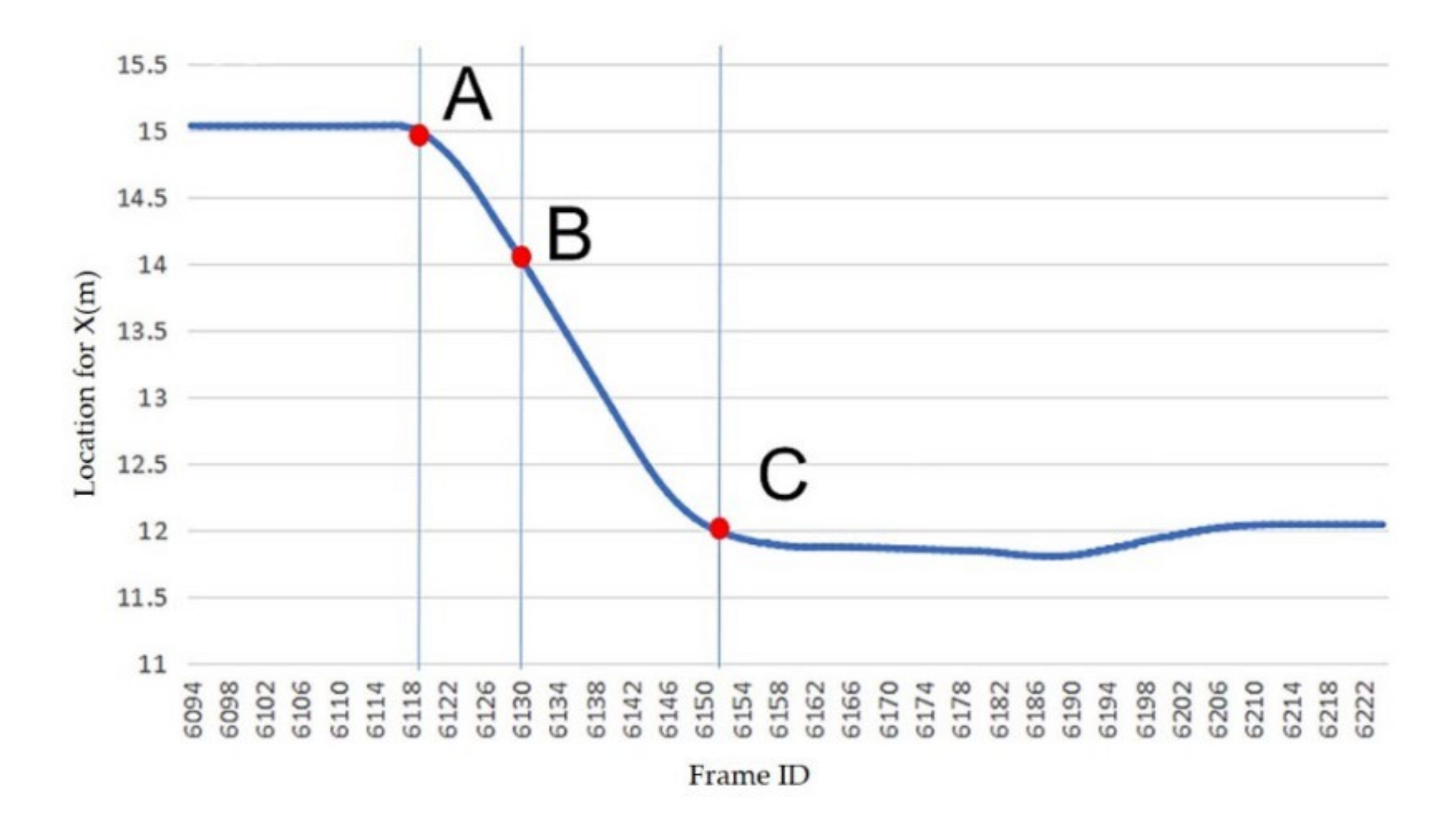
Vehicle operation trajectories are drawn according to the trajectory data set, and the entire lane-changing process of the vehicle is realized by marking the three crucial time nodes during the lane-changing process. The first time node, which belongs to the end of the lane change preparation stage and the start of the lane change execution stage, is the moment when the x coordinate of the vehicle changes greatly and is marked as A; the second time node, which is the end of the lane change execution stage and the start of the lane change adjustment stage, is the occurrence of the change in the ID of the lane where the driving vehicle is located and is denoted as B; the third time node, which is the end of the lane change adjustment stage, is the moment when the x coordinate of the driving vehicle tends to be stable and is denoted as C. Figure 2 is a schematic diagram of different stages and time nodes of the lane-changing procedure.

The three time points shown in Figure 2 divide the lane-changing behavior of vehicles into three phases. It is important to master the data characteristics of different phases. Here, MATLAB software (MATLAB version: 9.8.0.1323502 (R2020a); Creator: MathWorks; Location: America) is used to extract and process the trajectory data in the following steps.

Step 1: Extract all vehicle IDs that only change lanes once and store the trajectory data.

Step 2: Take the lane ID as the unit, store the trajectory data of the same vehicle before and after the lane-changing behavior, and record the last vehicle information after the lane-changing behavior as point B. Point B is at the end of the execution stage and the start point of the adjustment stage.

Step 3: Determine the end point of the lane change preparation stage, and record the end point as point A. The time period before A belongs to the lane change preparation stage, and the time period between A and B belongs to the lane change execution stage.

Step 4: Determine the end points of the lane change adjustment stage, and record the end point as point C. The time period between B and C belongs to the lane change adjustment stage.

After the time nodes at different stages of the vehicle lane-changing behavior are calibrated through the above identification steps, the corresponding lane-changing data can be extracted to provide a basic data set for research on lane-changing behavior.

3.2. Principal Component Analysis

Principal component analysis (PCA) is a classic statistical method. Through orthogonal transformation, a set of potentially correlated variables is transformed into a set of linearly uncorrelated variables (also called principal components). In practical applications, dimensions of irrelevant variables finally constructed are often fewer than the number of original variables. Therefore, the main variables with greater influence can be extracted and the complexity of the data would be simplified. Each variable is searched one by one and perform orthogonal transformation. Principal components are several larger variables obtained by orthogonal transformation, which are linear combinations of the original variables.

The study involves three stages (preparation stage, execution stage, and adjustment stage) in the lane-changing process, involving a total of n variables (vehicle speed, acceleration, distance, time distance, etc., in each stage), to establish a linear model of the longitudinal travel distance of the lane-changing behavior and the interrelated effects of variables. Because the variables may be correlated with each other, it is necessary to construct orthogonal variables to eliminate the correlation between them.

Firstly, raw data should be centered, which means unitedly adjusting the mean values to be 0. The original observed vehicle data have t different dimensional representations. The data for each x_i of the characteristic variables X_i have means of μ_i, which are obviously not all 0. To facilitate data dimensionality reduction and the use of variance to construct principal components, the data centering procedure adjust all the original sample data means to 0 to simplify the calculation of variance values. The variances of independent variables X_i are calculated by the following equation:

$$\begin{array}{l}Var(X_i)=Cov(X_i)=\frac{1}{n}{\displaystyle \sum _{i=1}^n{(x_i-{\mu }_i)}^2},\\ {\mu }_i=\frac{1}{n}{\displaystyle \sum _{i=1}^n{x}_i},i=1,2,\dots ,t.\end{array}$$

(1)

With the method, mean value of each variable μ_i = 0, the variance is:

$$\begin{array}{l}{\widehat{x}}_i=x_i-{\mu }_i,\\ Var(\widehat{X})=Cov(\widehat{X})=\frac{1}{n}{\displaystyle \sum _{i=1}^n{\widehat{x}}_i^2}\end{array}$$

(2)

This process is also the first step in finding the orthogonal basis: searching for the first base such that the variance value is maximized after transforming all data into the coordinate representation under the base.

Secondly, a covariance matrix needs to be constructed to characterize the degree of correlation between the two variables A, B in terms of covariance. After data centralization, the covariance formula is simplified:

$$\begin{array}{l}Cov(A_i,B_j)=\frac{1}{n}{\displaystyle \sum _{i=1}^n{a}_i{b}_j},\\ i,j=1,2,\dots ,t.\end{array}$$

(3)

Although the average coefficient of the unbiased mean and variance of the sample is 1/(n − 1), 1/n can be used to facilitate the calculation when the number of samples is large. After the orthogonal transformation of any two independent variables, the covariance of the two variables would be 0, which means no linear correlation after the procedure. Next, covariance matrices must be constructed for the two variables a_i, b_i and the arrangement of these two variables are represented with the matrix X:

$$X=\left(\begin{array}{l}{a}_1,a_2,\dots ,a_n\\ b_1,b_2,\dots ,b_n\end{array}\right)$$

(4)

The corresponding scatter matrix is XX^T, and the covariance matrix is (1/n) XX^T:

$$T=\frac{1}{n}X{X}^T=\left(\begin{array}{l}\frac{1}{n}{\displaystyle \sum _{i=1}^n{a}_i^2},\frac{1}{n}{\displaystyle \sum _{i=1}^n{a}_i{b}_i}\\ \frac{1}{n}{\displaystyle \sum _{i=1}^n{a}_i{b}_i},\frac{1}{n}{\displaystyle \sum _{i=1}^n{b}_i^2}\end{array}\right)=\left(\begin{array}{l}Var(A),Cov(A,B)\\ Cov(A,B),Var(B)\end{array}\right)$$

(5)

In order to orthogonalize any two variables, the covariance matrix should have 0 elements other than the diagonal positions, which means Cov(A, B) = 0. Therefore, the covariance matrix is diagonalized, which is the process of the eigenvalue decomposition. Based on the eigenvalue and eigenvector properties of the matrix, the following relationship equation is obtained:

$$T\overrightarrow{{\alpha }_i}={\lambda }_i\overrightarrow{{\alpha }_i}$$

(6)

The set of vectors is orthogonalized to obtain a set of unit vectors, and the matrix T is decomposed into the product of the diagonal matrix and the matrix of eigenvectors:

$$T=Q\sum Q^{-1}$$

(7)

where Σ is the diagonal matrix of eigenvalues λ_i arranged by size and Q is the matrix of corresponding eigenvectors $\overrightarrow{{\alpha }_i}$.

In general, for a matrix that is not square, T_m*n, the singular value decomposition method can be used:

$$T_{m*n}=U_{m*m}{\sum }_{m*n}{V}_{n*n}^{{}^T}$$

(8)

where the matrices U_m*m and V_n*n are orthogonal matrices and Σ_m*n is a matrix with all elements except the main diagonal element being singular.

Finally, to construct irrelevant variables and the representation of changes, use a matrix approach:

$$F=AX$$

(9)

where X is the original data representation and vector F is the new data representation.

$$\left(\begin{array}{l}{\overrightarrow{\alpha }}_1^T\\ {\stackrel{\rightharpoonup }{\alpha }}_2^T\\ ⋮\\ {\overrightarrow{\alpha }}_m^T\end{array}\right)\left({\overrightarrow{x}}_1,{\overrightarrow{x}}_2,\cdots ,{\overrightarrow{x}}_n\right)=\left(\begin{array}{l}{\overrightarrow{\alpha }}_1^T{\overrightarrow{x}}_1,{\overrightarrow{\alpha }}_1^T{\overrightarrow{x}}_2,\cdots ,{\overrightarrow{\alpha }}_1^T{\overrightarrow{x}}_n\\ {\overrightarrow{\alpha }}_2^T{\overrightarrow{x}}_1,{\overrightarrow{\alpha }}_2^T{\overrightarrow{x}}_2,\cdots ,{\overrightarrow{\alpha }}_2^T{\overrightarrow{x}}_n\\ ⋮\\ {\overrightarrow{\alpha }}_m^T{\overrightarrow{x}}_1,{\overrightarrow{\alpha }}_m^T{\overrightarrow{x}}_2,\cdots ,{\overrightarrow{\alpha }}_m^T{\overrightarrow{x}}_n\end{array}\right)$$

(10)

Among the functions, i = 1, 2, …, m, represents the ith mutually orthogonal basis and j = 1, 2, …, n, represents the original data and their dimensions are t. The next steps are to sort according to the corresponding eigenvalues, select according to the principle that the contribution rate needs to reach more than 85%, and obtain the final orthogonal variables for analysis, where m is the first m principal components selected.

After the PCA procedure, the principal component regression equation is required to be constructed according to the results. In the research, m characteristic indicators of the vehicle during the three steps of the lane-changing process are considered. When handling its correlation, a linear model is adopted to express this, which is represented by:

$$H={\displaystyle \sum _i{c}_i{x}_i},i=1,2,3,\dots ,m.$$

(11)

where H indicates the longitudinal driving distance of the lane-changing process, x_i indicates the influencing variables in the lane-changing process, and c_i indicates the weight of each variable. After the principal component analysis, the principal component regression equation for the longitudinal driving distance was constructed according to the percentage of the contribution of the principal components:

$$H={\displaystyle \sum _i{c}_i{\stackrel{⌢}{x}}_i},i=1,2,3,\dots ,n,n\le m.$$

(12)

3.3. Model Significance Test Method

After the model is constructed, it is necessary to judge the validity of the model. The research selects F-test and t-test methods to judge the model.

3.3.1. F-Test Method

To determine whether there is a linear relationship between the longitudinal travel distance H of the dependent variable and the independent variable, it is obvious that when the coefficient b_i of the independent variable (i = 1, 2, …, m, where m is the number of independent variables) is 0, the linear relationship is not conspicuous, so it is necessary to let the original hypothesis follows that:

$$H_0:{\mathrm{b}}_i=0,i=1,2,\dots ,m.$$

(13)

If H₀ holds, then the construction of the F-statistic gives:

$$F=\frac{SSR/m}{SSE/n-m-1}~F(m,n-m-1)$$

(14)

where SSR is the sum of squared regressions and SSE is the sum of squared residuals. At the significance level α, if F_1−α/2(m, n − m − 1) < F_α/2(m, n – m − 1), H₀ is accepted or otherwise rejected and indicates that the model fits well; thus, the overall correlation is significant and the model is reliable.

3.3.2. t-Test Method

F-test could only indicate that the coefficients of the model b_i are not all 0, but it is not possible to exclude the case that several of them are 0. Under the circumstance, t-test can test the significance of the coefficients of each variable in the model, so it is necessary to assume that:

$$H_0^{(i)}:b_i=0,i=0,1,\dots ,m.$$

(15)

When H⁽ⁱ⁾₀ holds, the statistic is:

$$t_i=\frac{b_i/\sqrt{b_{ii}}}{\sqrt{SSE/(n-m-1)}}\sim t(n-m-1)$$

(16)

where the symbolic meaning is the same as that of the above equation, b_ii is the (i, i) element in XX^T, and x_j1, x_j2, …, x_j18 (j = 1, 2, …, n.) are the observed values of x₁, x₂, …, x₁₈. At the confidence level α, if |t| < t_α/2(n − m − 1), then is accepted H⁽ⁱ⁾₀ and otherwise rejected, under which it indicates that the independent variable has a significant relationship with the dependent variable.

4. Case Study

4.1. Data Collection

A buffer zone in the lane adjacent to the dedicated lane for AVs can be set, where AVs can make preparations to change to the dedicated lane, and only once this is complete can the compulsive lane-changing procedure happen in the buffer zone. Since the dedicated lane for AV has not been implemented, it is difficult to collect the real lane-changing behavior trajectory data of AVs at the present time. For this reason, vehicle trajectory from the NGSIM data set was used to investigate the factors that influence the longitudinal driving distance of lane-changing behavior, so as to build a foundation to analyze the lane-changing behaviors in the buffer zones. The NGSIM trajectory data set for the I-80 highway in the United States was chosen for exploration in this experiment. The selected road section and direction includes a high occupancy vehicle lane, five regular lanes, and an on-ramp, which gives the highway section more lane-changing behaviors and facilitates the study of lane-changing behaviors. As indicated in Figure 3, each lane is approximately 3.5 m wide and the weather and pavement are in good condition. It could be deduced that the majority of lane-changing behaviors in the chosen section are forced because of the ramp, which corresponds to the lane-changing behavior features that were researched in the experiment. Only passenger vehicles are included in the research classification. MATLAB was used to extract the vehicle trajectory data to only include one-time lane changes.

There may be anomalous values and variations in the NGSIM because the indicators are instantaneous values recorded by frame. Preprocessing the original data, such as denoising and smoothing, is required to assure the reliability of the input data. First, data with null values in important indicators such as frame, speed, acceleration, vertical and horizontal position should be removed. Second, samples with excessive missing values or continuous missing indications are unfit for analysis and should be deleted. Finally, data smoothing can be adopted to deal with the circumstances where deviation is large. Data smoothing methods, such as the Kalman filter method [27], the moving average method [28], and the median filter method [29] are extensively employed. The moving average method is a statistical method that highlights trend characteristics by suppressing noise in the original data and dividing the change of the variable into trend and residual sections. The following is its general mathematical model:

$${\stackrel{⌢}{Y}}_i={\displaystyle \sum _{i=1}^n{W}_i{Y}_i}$$

(17)

where ${\stackrel{⌢}{Y}}_i$ is the calculated moving average value of the ith value in a group of data, Y_i is the ith data’s adjacent observation value, W_i is each observation value’s weighting coefficient, and n is the length of the window. Figure 4 shows the smoothing results of the vehicle’s acceleration. In addition, the same processing procedure is done for speed, relative lateral and longitudinal position, headway, and spacing.

4.2. Extraction of Information Related to Lane-Changing Behavior

The vehicle trajectory data including only one-time lane changes were extracted from the basic data set. The three stages of lane-changing behavior were calibrated. The preparation, execution, and adjustment stages of the vehicle lane-changing process are represented by these three-time nodes. A new data set was created from the vehicle speed, average acceleration, headway, spacing, and duration at each stage.

Table 1. Diagram of relevant variables.

Meaning of Variables	Variables	Meaning of Variables	Variables
Speed in preparation stage	X1	Duration in execution stage	X10
Average acceleration in preparation stage	X2	Speed in adjustment stage	X11
Spacing in preparation stage	X3	Average acceleration in adjustment stage	X12
Headway in preparation stage	X4	Spacing in adjustment stage	X13
Duration in preparation stage	X5	Headway in adjustment stage	X14
Speed in execution stage	X6	Duration in adjustment stage	X15
Average acceleration in execution stage	X7	Distance between target and rear vehicle	X16
Spacing in execution stage	X8	Rear vehicle speed in target lane	X17
Headway in execution stage	X9	Speed at the end of adjustment stage	X18

displays the extracted data.

As a result, 455 vehicles that only changed lanes once and 18 variables linked to the lane-changing procedure were extracted to assess the influencing factors of longitudinal driving distance during lane changes.

4.3. Analysis of Influencing Factors

AVs need to enter the dedicated lane through lane-changing behavior. Through progressive research in the field of ITS technology, it has been found that traditional single-vehicle intelligent technology makes it difficult to achieve full autonomous driving. Therefore, roadside infrastructure and road pavement markings are needed to help intelligent vehicles achieve autonomous driving functions in the initial stage of autonomous driving technology implementation. At the same time, AVs and HDVs will form a mixed traffic flow for a long time. In order to encourage the development of AVs and to ensure the efficiency of the mixed traffic flow, it is necessary to set up dedicated lanes for AVs on existing highways. Since AVs are randomly distributed in lanes before they enter the highway sections where the dedicated lane exists, AVs need to enter the dedicated lane through lane-changing behaviors. Setting a buffer zone in the adjacent lane can guarantee a safe lane change environment, as shown in Figure 5.

A buffer zone is a special section located adjacent to an autonomous driving dedicated lane that is closed to HDVs. The buffer zone can be set up as colored section of the pavement to facilitate recognition for AVs using computer vision. When the vehicle travels to the beginning of the buffer zone, the AV receives the lane change command and enters the lane change preparation stage. If the vehicle shows lateral displacement, it indicates that it has entered the execution stage. When the center of the vehicle crosses over to the dedicated lane, it indicates that it has entered the adjustment stage. The lane-changing behavior ends when there is no more lateral displacement of the vehicle. In the process of AVs driving into the dedicated lane, the buffer zone not only reminds and guides the vehicles into the dedicated lane, but also protects the AVs during the whole process of lane-changing behavior and avoids the interference of the HDVs. As a result, by studying the influencing factors of lane-changing behavior and exploring how to shorten the longitudinal distance of the lane-changing process, effective suggestions can be provided for setting the section length of the buffer zone.

To investigate the factors influencing lane-changing behavior, the authors used principal component analysis to process the lane-changing behavior data. SPSS was used to perform the principal component analysis of 455 standardized vehicles’ lane-changing information. Related factors are dimensionally reduced to obtain the correlation coefficient matrix, KMO Bartlett test, and principal component analysis results. Next, PCA results will be explained and the influencing factors of lane-changing behavior will be summarized.

First, the KMO Bartlett method was used to test the distribution and independence of the variables to determine the suitability of the data for PCA. The results of the KMO Bartlett test are shown in

Table 2. The results of the KMO Bartlett test.

KMO Bartlett Test
Kaiser–Meyer–Olkin measure of sampling adequacy		0.625
Bartlett’s sphericity test	Approximate chi square	3285.915
	df	153
	Sig.	0.000

. The KMO value is 0.625 and the Bartlett sphericity test statistic is 153, with a corresponding sig of 0.000, indicating a significant difference between the correlation coefficient matrix and the unit matrix. The data set is suitable for principal component analysis, according to Kaiser’s KMO measurement standard.

Next, PCA was performed on the lane-changing data for dimensionality reduction.

Table 3. Results of principal component analysis.

Composition	Characteristic Value	Variance Contribution Rate	Cumulative Contribution Rate
1	4.023	22.353	22.353
2	2.341	13.007	35.359
3	1.495	8.303	43.662
4	1.296	7.199	50.862
5	1.159	6.436	57.298
6	1.130	6.278	63.576
7	1.002	5.564	69.140
8	0.922	5.121	74.261
9	0.914	5.077	79.338
10	0.798	4.433	83.772
11	0.679	3.772	87.544

shows the results of principal component analysis. Based on the principle that the cumulative contribution rate should reach 85%, 11 major components were finally chosen for investigation.

Based on the results of PCA, the comprehensive score coefficient table of the filtered principal components was obtained and are shown in

Table 4. Comprehensive score coefficient table.

Variable	Composition
	F1	F2	F3	F4	F5	F6	F7	F8	F9	F10	F11
X1	0.68	−0.12	−0.09	0.07	0.21	−0.19	0.37	−0.47	0.04	0.05	0.03
X2	−0.05	0.69	0.24	−0.03	0.05	−0.23	−0.07	−0.07	0.42	0.31	−0.23
X3	0.45	−0.44	0.58	0.08	0.05	0.02	0.14	−0.33	0.11	0.11	0.15
X4	−0.08	−0.34	0.75	0.01	−0.19	0.27	−0.29	0.16	0.02	0.07	0.17
X5	−0.33	0.17	0.00	0.52	−0.37	−0.10	0.11	0.06	0.40	−0.02	0.34
X6	0.89	−0.02	−0.10	−0.03	−0.13	−0.10	−0.05	0.13	0.06	0.01	0.08
X7	−0.11	0.85	0.35	−0.13	0.09	−0.01	0.03	−0.06	0.05	0.08	−0.04
X8	0.42	−0.40	0.34	−0.11	0.11	0.08	0.09	0.13	0.15	0.00	−0.45
X9	0.00	0.03	−0.03	0.41	0.62	0.15	0.01	0.31	−0.23	0.49	0.12
X10	−0.26	−0.07	0.10	−0.01	−0.18	0.10	0.83	0.33	0.01	0.04	−0.05
X11	0.88	0.25	−0.04	−0.02	−0.15	−0.06	0.01	0.21	−0.02	0.06	0.09
X12	−0.17	0.56	0.37	−0.19	0.15	0.20	0.18	−0.17	−0.39	−0.29	0.18
X13	0.48	0.23	−0.11	−0.17	−0.04	0.51	−0.03	0.21	0.17	−0.12	−0.09
X14	−0.05	−0.03	−0.34	−0.24	0.09	0.67	0.03	−0.29	0.34	0.19	0.17
X15	−0.02	−0.13	0.03	−0.58	0.44	−0.31	0.05	0.32	0.31	−0.15	0.34
X16	0.16	0.13	0.06	0.59	0.42	0.16	−0.02	0.05	0.25	−0.52	−0.10
X17	0.77	0.08	0.03	0.06	0.03	−0.13	−0.10	0.02	−0.07	−0.06	0.15
X18	0.73	0.38	−0.02	0.07	−0.24	0.15	0.06	0.08	−0.17	0.05	0.05

. The factor load matrix of the associated standardized variable X_j (j = 1, 2, 3, …, 18) for the principal component F_i (i = 1, 2, 3, …, 11) is represented by the coefficient α_j (j = 1, 2, 3, …, 18) in the table.

The following is the calculating formula for each principal component:

$$F_i={\displaystyle \sum _{j=1}^{18}{\alpha }_j{X}_j}$$

(18)

The variance contribution rates provided by each principal component were selected as the weight to show the effect. Using the formula below, the sum of the variance contribution rates of the 11 principal components was expanded to 100 percent to calculate the weight coefficient of each principal component and the comprehensive score F:

$$F=0.255F_1+0.149F_2+0.095F_3+0.082F_4+0.074F_5+0.072F_6+0.064F_7+0.058F_8+0.058F_9+0.051F_{10}+0.043F_{11}$$

(19)

Finally, the analysis of comprehensive score coefficient for variables, shown in Table 4, allows explanation of the 11 principal component. As shown in

Table 5. Explanations for each principal component.

Principal Component	Definition
1	Speed index
2	Vehicle stability index
3	Flow index (preparation stage in buffer zone)
4	Duration index (preparation and execution stages)
5	Duration index (adjustment stage)
6	Flow index (adjustment stage)
7	Duration index (execution stage)
8	Duration index (execution and adjustment stages)
9	Stability index
10	Flow index (execution stage in dedicated lane)
11	Duration index (preparation and adjustment stages)

, the meaning of each principal component can be interpreted and defined according to the composition of different variables.

F₁ can be interpreted as the speed index. The load proportion of the main variables X₁, X₆, X₁₁, X₁₇, and X₁₈ are the largest ones, which represent the speed of the lane-changing vehicle in the preparation, execution, and adjustment stages, and the rear vehicle speed in the target lane and the final speed in the lane-changing process, as can be seen from the expression of the first principal component F₁. It shows that the speed of vehicle changing lanes and the rear vehicle has a great impact during the process of lane changing.

F₂ can be understood as the vehicle stability index for the entire lane-changing process. In the second principal component, X₂, X₇, and X₁₂ have the largest load proportion. The average acceleration of lane-changing vehicles during the preparation, execution, and adjustment stages is represented by these three variables. F₃ represents the flow index of the buffer zone in the lane change preparation stage, where variables X₃ and X₄ account for the largest load proportion.

Similarly, for duration indexes, the fourth principal component, F₄, represents the duration index of the previous two stages during the lane-changing procedure, F₈ represents the duration index of the last two stages, and F₁₁ is the duration index of the preparation and adjustment stages. Moreover, F₅ indicates the duration index of the adjustment stage and F₇ represents the duration index of the execution stage. As for flow indexes, F₆ is the dedicated lane flow index of the adjustment stage and F₁₀ represents the dedicated lane flow index of the execution stage. In addition, F₉ is the stability index of the preparation and adjustment stages.

4.4. Model Construction and Model Testing

The primary influencing elements in the process of lane-changing were examined in the preceding section. The principal component must be treated as a variable in order to analyze the longitudinal driving distance throughout the entire process of lane-changing behavior. The factor score result needs to be transformed into the main component score result through the formula:

$$f_{ij}=Fa{c}_{ij}\times \sqrt{{\eta }_j}$$

(20)

where f_ij represents the principal component score, Fac_ij represents the factor score, and n_j represents the eigenvalue of the corresponding principal component. Based on the principal component score results, linear regression modeling is built. The collected 11 main components are independent variables, while the longitudinal distance in the lane-changing process is the dependent variable. The longitudinal driving distance H in the lane-changing process can be modeled using a principal component regression model. The following is the model equation:

$$H=-0.032f_1+0.058f_2+0.025f_3+0.358f_4-0.251f_5-0.142f_6+0.298f_7+0.135f_8+0.405f_9-0.094f_{10}+0.519f_{11}$$

(21)

4.4.1. F-Test

The significance test of the model, the F-test, should be performed before the significance test of each regression coefficient in the multiple linear regression model, as indicated in

Table 6. F-test for the model.

Model	Sum of Squares	df	Mean Square	F	Sig.
Regression	326.946	11	29.722	103.634	0.000
Residual	127.054	443	0.287
Total	454.000	454

.

When the significance level is 0.05, statistic $F=103.634\notin \left(0.345, 2.022\right)$, so the original hypothesis is rejected. The test resulted in the longitudinal driving distance influence model of lane-changing passing. It shows that the model fits well, the overall correlation is significant, and the model is reliable.

4.4.2. t-Test

The F-test yielded a significant result. However, it does not imply that each explanatory variable has a significant effect on the explained variable. As a result, the significance of each variable’s coefficient must be tested using the t-test, as indicated in

Table 7. Principal component linear regression coefficient.

Model	Non-Standardized Coefficient		Standardized Coefficient	t	Sig.
	B	Standard Error
(Constant)	0.000	0.025		0.000	1.000
f1	−0.032	0.013	−0.064	−3.336	0.002
f2	0.058	0.016	0.089	3.542	0.000
f3	0.025	0.021	0.030	1.195	0.233
f4	0.358	0.022	0.407	16.202	0.000
f5	−0.251	0.023	−0.270	−10.753	0.000
f6	−0.142	0.024	−0.151	−6.014	0.000
f7	0.298	0.025	0.298	11.865	0.000
f8	0.135	0.026	0.129	5.139	0.000
f9	0.405	0.026	0.387	15.405	0.000
f10	−0.094	0.028	−0.084	−3.355	0.001
f11	0.519	0.031	0.428	17.015	0.000

:

The model coefficients other than b₀ and b₃ are highly significant when the significance level is 0.05, indicating that headway and spacing in the preparation stage are not significant, whereas speed, acceleration, and duration time are significantly related to the longitudinal driving distance of lane-changing behavior.

5. Results

5.1. Comparative Analysis

The validity of the longitudinal driving distance model was demonstrated by the PCA model test results. As demonstrated in the following section, SPSS was used to create a general linear regression equation for the standardized variables on the longitudinal driving distance of lane-changing behavior, which was then compared to the results of PCA to confirm the validity of the model.

To begin, the R-square values of the two models were compared (see

Table 8. Comparison of R² and standard estimation error of two models.

Model	R	R2	Adjusted R2	Standard Estimation Error
PC Linear Regression	0.849	0.720	0.713	0.536
General Linear Regression	0.895	0.801	0.793	59.399

). The R-square result of the general linear regression model is slightly better than the PCA model. The model’s fitting effect is influenced by the fact that some independent variables are abandoned in the process of PCA. The error of PCA estimation to the real value is smaller, which means a higher practical value. However, R-square and standard estimation error cannot comprehensively evaluate the model’s fitting effect. It is therefore required to assess both the model’s overall fitting degree and the significance test of independent variables.

An integrity test was added to the general linear regression equation (as shown in

Table 9. F-Test of general linear regression model.

Model	Sum of Squares	df	Mean Square	F	Sig.
Regression	6,204,802.725	18	344,711.262	97.700	0.000
Residual	1,538,326.007	436	3528.271
Total	7,743,128.732	454

). Its statistic $F=97.7\notin \left(0.345, 2.022\right)$, which passes the hypothesis test and means the general linear regression model equation generally fits well.

However, when each coefficient was tested using a t-test with a significance level of 0.05 (as shown in

Table 10. Coefficient and significance of general linear regression.

Variable	Coefficient	t	Sig.	Variable	Coefficient	t	Sig.
(Constant)	−94.186	−5.469	0.000	X10	7.642	8.370	0.000
X1	1.713	3.478	0.001	X11	1.171	1.498	0.135
X2	−31.998	−3.656	0.000	X12	−2.138	−0.332	0.740
X3	0.028	0.242	0.809	X13	−0.268	−2.750	0.006
X4	4.334	1.559	0.120	X14	0.103	0.206	0.837
X5	4.388	37.124	0.000	X15	5.522	7.608	0.000
X6	2.470	3.907	0.000	X16	0.685	4.010	0.000
X7	16.633	1.895	0.059	X17	−0.427	−1.071	0.285
X8	−0.183	−2.245	0.025	X18	0.118	0.227	0.820
X9	−0.005	−0.786	0.432

), 11 coefficients failed the test, indicating that the established PCA model is more effective than the general linear regression model.

In summary, the PCA regression model of longitudinal travel distance for lane changes is more practical than the general linear regression model and can estimate and predict the longitudinal driving distance for a series of indicators in the process of lane changes.

5.2. Discussion

The longitudinal driving distance of the lane-changing process is in negative correlation with the speed of the lane-changing process, meaning that the faster the lane-changing vehicle, the shorter the longitudinal driving distance, as well as the acceleration. This finding indicates that maintaining vehicle stability can reduce the length of the buffer zone. The distance increases when the first two stages of lane-changing progress are extended. The fifth principal component demonstrates that the whole driving distance could be effectively reduced by increasing the time proportion of the adjustment stage. The coefficients of the sixth and tenth principal components are negative, which means that the longitudinal driving distance of the lane-changing process becomes longer as the traffic volume of the dedicated lane increases during the execution and adjustment stages. The remaining key components in the lane-changing process are related to lane change duration and acceleration, demonstrating that preserving vehicle stability and reducing lane change duration time shortens the longitudinal driving distance.

In the study by Huang et al. [12], they studied the factors influencing the lane change spacing from a macroscopic perspective. They selected traffic flow, the proportion of lane-changing vehicles, the average speed of vehicles within the roadway, and the travel time during the lane-changing process as the variables of their study. On the contrary, this current work investigates the vehicle micro-trajectory data to study the influencing factors of lane-changing behavior. Factors such as headway, spacing, speed, acceleration, and duration during different lane-changing stages were investigated. Figure 6 illustrates the five factors that influence lane-changing phenomenon. From a microscopic perspective, both spacing and headway can reflect the traffic flow to some extent. The increase in spacing and headway means that the traffic flow in the target lane is smaller, which helps to improve the efficiency of lane-changing behavior. When the speed of the target vehicle is consistent with the driving speed in the target lane, it contributes to the fast completion of the lane-changing behavior. The acceleration of the target vehicle reflects the driving stability of the vehicle, and the reduction of acceleration is beneficial to the efficiency and safety of the lane-changing behavior. The duration was divided into three stages. The analysis in Section 5.1 shows that the lower the proportion of duration in the preparation stage, the more efficient the lane-changing behavior. In this paper, the efficiency of the lane-changing behavior is expressed in terms of the longitudinal driving distance. Therefore, efficient lane-changing behavior will lead to a reduction in the longitudinal driving distance, which means the length of the buffer zone can be reduced.

In regard to the lane change spacing, Huang et al. [12] concluded that, when the traffic flow and the ratio of lane-changing vehicles are increased, the required lane change spacing increases, which means that the longitudinal distance of lane-changing behavior increases. Meanwhile, they argue that the longitudinal distance can be reduced when the traffic speed is increased and when the duration of the lane-changing behavior increases, the longitudinal driving distance also increases, which is negative to the traffic capacity. Their results showed that the longitudinal distance for the lane-changing behavior is shorter when the design speed difference between two lanes is smaller and the speed is higher. Additionally, when the headway distance of the target lane is large, it can help to reduce the longitudinal driving distance. Finally, reducing the percentage of duration in the preparation stage will also effectively shorten the longitudinal driving distance. A comparison reveals that the paper draws the same conclusions as the related literature. The work refines the lane-changing behavior into three stages and pinpoints one of the factors influencing the longitudinal driving distance as the lane change preparation stage.

To summarize, when determining the length of the buffer zone, speed, acceleration, and traffic flow in the dedicated lane must all be considered. Additionally, the length of the longitudinal driving distance will be affected by the proportion of time spent in each of the three stages during the lane-changing process. As a result, while defining the length of the dedicated lane’s buffer zone, we recommend setting the design speed of the buffer zone to the same level as the dedicated lane. The driving stability of vehicles should also be guaranteed. The headway and spacing of AVs on the dedicated lane should be appropriately adjusted to increase the efficiency of vehicles entering the dedicated lane and reduce the buffer zone’s fixed length.

6. Conclusions

Using the NGSIM data set in this paper, the authors analyzed the influencing factors of lane-changing behavior, summarized various factors in the lane-changing procedure by using the dimensionality reduction method, and discussed the setting of the buffer zone length by analyzing the principal component regression model in order to provide theoretical support for the autonomous driving dedicated lane-setting scheme in the future. The length of the buffer zone is shown to be influenced by vehicle speed while changing lanes. The method of improving the design speed of the buffer zone can be considered to reduce the length of the buffer zone. Simultaneously, the acceleration of the lane-changing vehicles should be as stable as possible, and the proportion of time spent in the preparation stage must be reduced. Finally, keeping the dedicated lane relatively sparsely spaced is more conducive to improving lane-changing efficiency. The basic design of autonomous driving dedicated lanes holds an important place in the development of autonomous driving technology. The buffer zone is designed to provide a lane change alert area for AVs to drive into the dedicated lane. It also ensures safety during the lane-changing process and separates AVs from HDVs. Based on the microscopic trajectory data, we analyzed the factors influencing the longitudinal driving distance of the lane-changing procedure, which also affect the length of the buffer zone. This paper will serve as a theoretical guide in road design related to autonomous driving technology.

The work contained in this paper also has some limitations. The trajectory data used are from NGSIM human-driven vehicles, which cannot totally reconstruct AVs’ lane-changing characteristics. The consideration of buffer zone length is still under theoretical analysis due to the difficulty of creating a longitudinal driving distance model for AVs’ lane-changing behavior. When the technological conditions are more mature, the quantitative analysis of autonomous vehicle lane changes will be more complete and have a refining effect on this study.

References

1. Jin, S.; Sun, D.-H.; Zhao, M.; Li, Y.; Chen, J. Modeling and stability analysis of mixed traffic with conventional and connected automated vehicles from cyber physical perspective. Phys. A Stat. Mech. Its Appl. 2020, 551, 124217. [Google Scholar] [CrossRef]
2. Vander Laan, Z.; Sadabadi, K.F. Operational performance of a congested corridor with lanes dedicated to autonomous vehicle traffic. Int. J. Transp. Sci. Technol. 2017, 6, 42–52. [Google Scholar] [CrossRef]
3. Kumar, A.; Guhathakurta, S.; Venkatachalam, S. When and where should there be dedicated lanes under mixed traffic of automated and human-driven vehicles for system-level benefits? Res. Transp. Bus. Manag. 2020, 36, 100527. [Google Scholar] [CrossRef]
4. Gipps, P.G. A model for the structure of lane-changing decisions. Transp. Res. Part B Methodol. 1986, 20, 403–414. [Google Scholar] [CrossRef]
5. Ahmed, K.I. Modeling Drivers’ Acceleration and Lane Changing Behavior; Massachusetts Institute of Technology: Cambridge, MA. USA, 1999. [Google Scholar]
6. Toledo, T.; Katz, R. State dependence in lane-changing models. Transp. Res. Rec. 2009, 2124, 81–88. [Google Scholar] [CrossRef] [Green Version]
7. Kesting, A.; Treiber, M.; Helbing, D. General lane-changing model MOBIL for car-following models. Transp. Res. Rec. 2007, 1999, 86–94. [Google Scholar] [CrossRef] [Green Version]
8. Zhao, D.; Peng, H.; Nobukawa, K.; Bao, S.; LeBlanc, D.J.; Pan, C.S. Analysis of mandatory and discretionary lane change behaviors for heavy trucks. arXiv 2017, arXiv:1707.09411. [Google Scholar]
9. Balal, E.; Cheu, R.L.; Gyan-Sarkodie, T.; Miramontes, J. Analysis of discretionary lane changing parameters on freeways. Int. J. Transp. Sci. Technol. 2014, 3, 277–296. [Google Scholar] [CrossRef] [Green Version]
10. Peng, J.; Guo, Y.; Fu, R.; Yuan, W.; Wang, C. Multi-parameter prediction of drivers’ lane-changing behaviour with neural network model. Appl. Ergon. 2015, 50, 207–217. [Google Scholar] [CrossRef]
11. Ataelmanan, H.; Puan, O.; Hassan, S. Empirical Evaluation of Lane Changing Following Gap Distance on Expressway. IOP Conf. Ser. Mater. Sci. Eng. 2021, 1144, 012077. [Google Scholar] [CrossRef]
12. Huang, Z.; Zhang, Z.; Li, H.; Qin, L.; Rong, J. Determining appropriate lane-changing spacing for off-ramp areas of urban expressways. Sustainability 2019, 11, 2087. [Google Scholar] [CrossRef] [Green Version]
13. Gu, X.; Abdel-Aty, M.; Xiang, Q.; Cai, Q.; Yuan, J. Utilizing UAV video data for in-depth analysis of drivers’ crash risk at interchange merging areas. Accid. Anal. Prev. 2019, 123, 159–169. [Google Scholar] [CrossRef]
14. Toledo, T.; Zohar, D. Modeling duration of lane changes. Transp. Res. Rec. 2007, 1999, 71–78. [Google Scholar] [CrossRef]
15. Franco, B.; Álvaro, C.; Francisca, C.-P.; Raúl, P.; Mauricio, V. Assessing influential factors for lane change behavior using full real-world vehicle-by-vehicle data. Transp. Lett. 2022, in press. [CrossRef]
16. Shi, J.; Liu, M. Impacts of differentiated per-lane speed limit on lane changing behaviour: A driving simulator-based study. Transp. Res. Part F Traffic Psychol. Behav. 2019, 60, 93–104. [Google Scholar] [CrossRef]
17. Chen, T.; Shi, X.; Wong, Y.D. Key feature selection and risk prediction for lane-changing behaviors based on vehicles’ trajectory data. Accid. Anal. Prev. 2019, 129, 156–169. [Google Scholar] [CrossRef]
18. Chauhan, P.; Kanagaraj, V.; Asaithambi, G. Understanding the mechanism of lane changing process and dynamics using microscopic traffic data. Phys. A Stat. Mech. Its Appl. 2022, 593, 126981. [Google Scholar] [CrossRef]
19. Hang, J.; Yan, X.; Ma, L.; Duan, K.; Zhang, Y. Exploring the effects of the location of the lane-end sign and traffic volume on multistage lane-changing behaviors in work zone areas: A driving simulator-based study. Transp. Res. Part F Traffic Psychol. Behav. 2018, 58, 980–993. [Google Scholar] [CrossRef]
20. Yuan, J.; Abdel-Aty, M.; Cai, Q.; Lee, J. Investigating drivers’ mandatory lane change behavior on the weaving section of freeway with managed lanes: A driving simulator study. Transp. Res. Part F: Traffic Psychol. Behav. 2019, 62, 11–32. [Google Scholar] [CrossRef]
21. Chen, Z.; Zhang, Y.; Wu, C.; Ran, B. Understanding Individualization Driving States via Latent Dirichlet Allocation Model. IEEE Intell. Transp. Syst. Mag. 2019, 11, 41–53. [Google Scholar] [CrossRef]
22. Li, G.; Chen, Y.; Cao, D.; Qu, X.; Cheng, B.; Li, K. Extraction of descriptive driving patterns from driving data using unsupervised algorithms. Mech. Syst. Signal Process. 2021, 156, 107589. [Google Scholar] [CrossRef]
23. Chen, Y.; Dong, C.; Palanisamy, P.; Mudalige, P.; Muelling, K.; Dolan, J.M. Attention-based hierarchical deep reinforcement learning for lane change behaviors in autonomous driving. In Proceedings of the IEEE/CVF Conference on Computer Vision and Pattern Recognition Workshops, Long Beach, CA, USA, 16–17 June 2019. [Google Scholar]
24. Yang, D.; Zheng, S.; Wen, C.; Jin, P.J.; Ran, B. A dynamic lane-changing trajectory planning model for automated vehicles. Transp. Res. Part C Emerg. Technol. 2018, 95, 228–247. [Google Scholar] [CrossRef]
25. Gu, X.; Han, Y.; Yu, J. A novel lane-changing decision model for autonomous vehicles based on deep autoencoder network and XGBoost. IEEE Access 2020, 8, 9846–9863. [Google Scholar] [CrossRef]
26. Ali, Y.; Zheng, Z.; Haque, M.M.; Wang, M. A game theory-based approach for modelling mandatory lane-changing behaviour in a connected environment. Transp. Res. Part C Emerg. Technol. 2019, 106, 220–242. [Google Scholar] [CrossRef]
27. Rempe, F.; Franeck, P.; Fastenrath, U.; Bogenberger, K. A phase-based smoothing method for accurate traffic speed estimation with floating car data. Transp. Res. Part C Emerg. Technol. 2017, 85, 644–663. [Google Scholar] [CrossRef]
28. Xin, P.; Liu, Y.; Yang, N.; Song, X.; Huang, Y. Probability distribution of wind power volatility based on the moving average method and improved nonparametric kernel density estimation. Glob. Energy Interconnect. 2020, 3, 247–258. [Google Scholar] [CrossRef]
29. Zhang, J. An efficient median filter based method for removing random-valued impulse noise. Digit. Signal Process. 2010, 20, 1010–1018. [Google Scholar] [CrossRef]
Figure 1. The layout of the dedicated lane and the buffer zone.
Applsci 12 04923 g001
Figure 2. Key time nodes for lane-changing behavior recognition.
Applsci 12 04923 g002
Figure 3. I-80 highway segment lane layout diagram.
Applsci 12 04923 g003
Figure 4. Diagram of vehicle trajectory data smoothing (acceleration as an example).
Applsci 12 04923 g004
Figure 5. Diagram of the buffer zone for lane-changing behavior.
Applsci 12 04923 g005
Figure 6. The influencing factors of the lane-changing phenomenon.
Applsci 12 04923 g006