Article

Dynamic Anchor: A Feature-Guided Anchor Strategy for Object Detection

School of Resources and Environment, University of Electronic Science and Technology of China, Chengdu 611731, China
*
Author to whom correspondence should be addressed.
Appl. Sci. 2022, 12(10), 4897; https://doi.org/10.3390/app12104897
Submission received: 4 March 2022 / Revised: 30 April 2022 / Accepted: 3 May 2022 / Published: 12 May 2022
(This article belongs to the Topic Applied Computer Vision and Pattern Recognition)

Abstract

:
The majority of modern object detectors rely on a set of pre-defined anchor boxes, which enhances detection performance dramatically. Nevertheless, the pre-defined anchor strategy suffers some drawbacks, especially the complex hyper-parameters of anchors, seriously affecting detection performance. In this paper, we propose a feature-guided anchor generation method named dynamic anchor. Dynamic anchor mainly includes two structures: the anchor generator and the feature enhancement module. The anchor generator leverages semantic features to predict optimized anchor shapes at the locations where the objects are likely to exist in the feature maps; by converting the predicted shape maps into location offsets, the feature enhancement module uses the high-quality anchors to improve detection performance. Compared with the hand-designed anchor scheme, dynamic anchor discards all pre-defined boxes and avoids complex hyper-parameters. In addition, only one anchor box is predicted for each location, which dramatically reduces calculation. With ResNet-50 and ResNet-101 as the backbone of the one-stage detector RetinaNet, dynamic anchor achieved 2.1 AP and 1.0 AP gains, respectively. The proposed dynamic anchor strategy can be easily integrated into the anchor-based detectors to replace the traditional pre-defined anchor scheme.

1. Introduction

As a fundamental and challenging branch of computer vision, object detection aims to predict a set of boxes with categories for all instance in an image [1,2,3]. The pre-existing domain-specific image object detectors can be divided into two categories: one is anchor-based detectors, such as Faster R-CNN [4], YOLOv2 [5], YOLOv3 [6], SSD [7], RetinaNet [8], etc.; and the other is anchor-free detectors, including YOLOv1 [9], DenseBox [10], Unitbox [11], CornerNet [12], FSAF [13], CenterNet [14], FoveaBox [15], etc.
Anchor-based detectors usually tile a set of pre-defined anchors on the image, set as reference boxes for all objects. The scales and aspect ratios of anchors are obtained by clustering or manual design for a specific dataset. The detectors first assign anchors to different ground-truth bounding boxes based on the traditional intersection-over-union (IoU) sample selection strategy in training, followed by predicting the category and refining the coordinates of these anchors one or several times. The detectors decode regression offsets with corresponding anchors during testing and produce refined anchors as detection results. The anchor-based detectors still achieve state-of-the-art detection performance at this time.
As mentioned in previous works [16,17,18], the pre-defined anchor strategy has some flaws: (1) the anchor boxes involve a considerable number of calculations, such as calculating IoU scores with ground-truth boxes; (2) hyper-parameters, including the scales, aspect ratios and number of anchors, are related to the dataset. Hyper-parameters also need to be redesigned for different tasks, which limits the generalization ability of the algorithm. Meanwhile, these hyper-parameters severely affect the detector’s performance; (3) as anchors’ scales and aspect ratios are fixed, detectors encounter difficulties when detecting objects with significant shape variations.
To mitigate the above problems of the pre-defined anchor scheme, we propose a more straightforward and more effective method to generate anchor boxes. Our approach is inspired by the fact that anchor-based detectors usually use an IoU threshold to select the positive anchors. As shown in Figure 1, we show a group of anchor boxes. For each point on the feature map, the pre-defined anchor strategy sets three sizes of anchor boxes, and the aspect ratios of anchors are also set to three types, including 1:1, 1:2, and 2:1. Therefore, nine anchor boxes are placed on each feature point. For an image with a size of 608 × 608, the number of pre-defined anchors has reached an amazing 69K. In the training, by setting the threshold (usually 0.4 and 0.5) and calculating the intersection-over-union scores between anchor boxes and ground-truth boxes, we assign anchors to each ground-truth box. Most of the anchors will not match the ground-truth box, as their IoU scores are lower than 0.4, as shown in Figure 1c. Then, a large number of negative anchors participate in classification loss calculation, which will cause a serious imbalance between the positive and negative samples. In the heads of detectors, the model will regress the offsets of the matched anchor box and the ground-truth box, and anchors with higher scores are easier to regress and obtain more accurate predictions. Therefore, improving the IoU scores of the anchor boxes can obtain more positive candidate boxes and lead to more accessible box regression. At the same time, reducing the number of anchor boxes is conducive to improving reasoning speed and reducing the requirements of computing resources.
As the optimal anchor box of an object is related to its features, the detectors attempt to predict the shapes of anchor boxes with feature maps. According to the above analysis, our method prepares anchor boxes in two steps: assigning the ground-truth boxes to different feature levels and selecting positive locations in the feature maps for anchor shape predictions; and determining the shape targets of the anchor boxes at different positions, with the anchor boxes achieving the maximum IoU scores with the ground-truth boxes. After obtaining a set of high-quality predicted anchor boxes, we propose the feature enhancement module to enhance the semantic features of the objects and develop detection performance.
We implement the dynamic anchor on RetinaNet (DA-RetinaNet) with the anchor generator and the feature enhancement module. The anchor generator uses the feature maps from the feature pyramid (FPN [19]) to predict the optimal anchor shapes without any pre-defined boxes. Therefore, DA-RetinaNet avoids all hyper-parameters of the anchor boxes. In addition, as the scales and aspect ratios of the anchor boxes are learnable rather than fixed, the detector makes it easier to handle tall or wide objects. In the experiments, the predicted anchors as the detection results achieved 26.5% Average Precision (AP) on COCO2017 minival, proving the effectiveness of our scheme. The proposed dynamic anchor can lead to significant improvements on the anchor-based detectors. On COCO test-dev [20], DA-RetinaNet improved AP by 2.1% while using ResNet-50 [21] as the backbone, and DA-RetinaNet achieved 40% AP with ResNet-101, outperforming the baseline and guided anchoring [22]. The main contributions of this paper can be summarized as follow:
  • We propose an alternative anchor strategy (dynamic anchor) to automatically generate anchor boxes without any hyper-parameters. Compared with the pre-defined anchor scheme, dynamic anchor would generate anchor boxes that are specific to the objects and avoid careful parameter tuning;
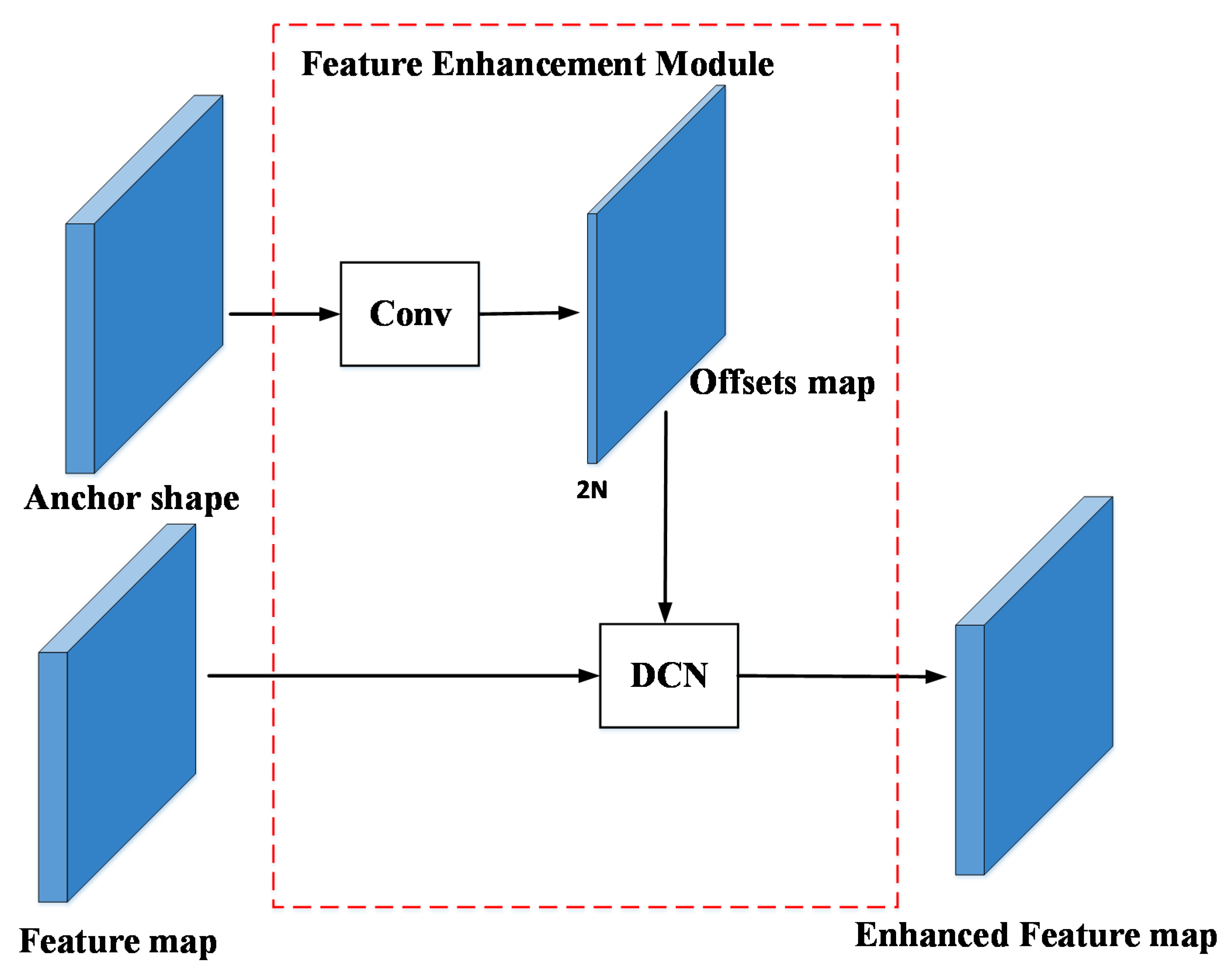
  • We propose a feature enhancement module, which takes advantage of the high IoU scores of the predicted anchors. The module enables the network to focus on the region of anchors and extract more precise semantic features;
  • We propose a quality branch, which is used to predict the quality scores of the predicted anchors. By investigating the influence of the anchor boxes with different quality, the scores are used to repress the low-quality anchors. The code will be available at https://github.com/LX-SZY/Dynamic-Anchor (accessed on 3 March 2022).

2. Related Work

Anchor-based detectors: Faster R-CNN [4] first demonstrated the method of employing anchor boxes to detect objects, inspired by the traditional sliding-window and proposal-based detectors. After that, the anchor boxes with fixed scales and aspect ratios were widely used in modern object detectors. The anchor boxes are regarded as reference boxes or proposal boxes in single-stage detectors [5,6,8,23,24,25]. SSD [7] utilizes the feature maps from multi-layers to detect objects with different scales. YOLOv2 [5] applies the anchors for classification and box regression to achieve better performance than YOLOv1 [9]. RetinaNet [8] proposes focal loss to mitigate the classification imbalance problem. Compared with single-stage detectors, two-stage or multi-stage detectors [4,26] usually implement the Region Proposal Network (RPN) to generate regions of interests (RoIs). Then, RoI Pooling and RoI Align layers are used to extract aligned features of the RoI. In addition, several detectors [24,27,28] adopt a cascade layer to refine detection bounding boxes step by step.
Refined anchor-based detectors: In recent years, a large number of works have aimed to improve the pre-defined anchor strategy. For the anchor assignment strategy, ATSS [17] acquires the IoU scores of the anchor boxes near the ground-truth box and calculates the mean and variance to determine the IoU threshold of each bounding box adaptively. PAA [29] separates the anchors into positive and negative samples for the ground-truth boxes according to the learning status of the model. For the anchor generation strategy, MetaAnchor [30] proposes an anchor function to generate anchor boxes from the arbitrary customized prior boxes dynamically. Guided Anchor [22] refines basic boxes with the shape prediction branch Based on the pre-defined anchor boxes.

3. Dynamic Anchor

As shown in Figure 2, this section first establishes an optimization equation and proposes an anchor generator for predicting the optimal anchor shape for each location. Next, we show the feature enhancement module, which utilizes the predicted anchors to improve detection performance. Finally, we present the quality branch, which helps suppress the low-quality anchor boxes.

3.1. Anchor Generator

3.1.1. Anchor Shape Targets

As shown in Figure 3a, the pre-defined anchor box B = x , y , w , h is assigned as a positive sample for the ground-truth box GT = x g t , y g t , w g t , h g t The distances from the central location x , y to the four sides of GT are l, t, r, and b, respectively. As the width and height of B are empiric values, we believe that there is an anchor box B * = x , y , w * , h * with the same center x , y in theory, and the box B * satisfies the condition: I o U B * , GT > I o U B , GT . IoU means calculating the intersection over the union of two rectangle boxes, as:
I o U b o x 1 , b o x 2 = b o x 1 b o x 2 b o x 1 b o x 2
Therefore, the critical issue is to determine the values of w * and h * , which can lead to the highest IoU score with the ground-truth box GT. The optimization equation is established as follows:
max : I o U x , y , w * , h * ,   x g t , y g t , w g t , h g t
s . t . w g t w * 2 r
h g t h * 2 b
where w * and h * are variables to be optimized. To maintain the consistency of the shape targets, the restriction conditions are set to w g t w * and h g t h * . In fact, if we set 0 w * and 0 h * , we will obtain two types of anchor box solutions. One is smaller than the ground-truth box, and the other is larger than the ground-truth box. Since the small anchor box is not conducive to subsequent feature enhancement, the limiting condition is set to w g t w * and h g t h * . By transforming Equation (2) into the form of an optimization equation, we obtain Equation (3):
min f w * , h * = [ w * · h * + w g t · h g t w * 2 + l · h * 2 + t ] / [ w * 2 + l · h * 2 + t ] s . t . w g t w * 0
w * 2 r 0
h g t h * 0 h * 2 b 0
Assuming that there are optimal solutions to Equation (3), and there are parameters defined as, λ1, λ2, λ3, λ4, satisfying the following KKT conditions:
h * · w * 2 + l 1 2 w * · h * + w g t · h g t / w * 2 + l 2 · h * 2 + t   +   λ 2   λ 1 = 0 w * · h * 2 + t 1 2 w * · h * + w g t · h g t / w * 2 + l · h * 2 + t 2   +   λ 4   λ 3 = 0   λ 1 · w g t w = 0   λ 2 · w 2 r = 0   λ 3 · h g t h = 0   λ 4 · h 2 b = 0   λ i 0   i = 1 ,   2 ,   3 ,   4
By solving Equation (4), we obtain five sets of solutions, both feasible and infeasible. The solutions are as follows:
Feasible solutions:
Solution   1 :   w * = w g t · h g t / 2 t h * = w g t · h g t / 2 l   λ 1 = λ 2 = λ 3 = λ 4 = 0
Solution   2 : w * = 2 r h * = 2 b   λ 1 = λ 3 = 0   λ 2 = ( w g t · h g t 4 b · l ) / 2 · w g t 2 · h g t   λ 4 = ( w g t · h g t 4 r · t ) / 2 · w g t · h g t 2
Solution   3 : w * = w g t h * = h g t   λ 2 = λ 4 = 0   λ 1 = h g t · 2 l w g t / ( h g t + 2 t · w g t / 2 + l 2 )   λ 2 = w g t · 2 t h g t / ( w g t + 2 l · h g t / 2 + t 2 )
Infeasible Solutions:
  Solution   4 : w * = 2 r h * = h g t   λ 1 = λ 4 = 0   λ 2 = h g t · 2 r w g t / ( h g t + 2 t · w g t 2 )   λ 3 = 2 r t w g t · h g t / 2 / ( w g t · h g t / 2 + t 2 )
Solution   5 : w * = w g t h * = 2 b   λ 2 = λ 3 = 0   λ 1 = 2 b l w g t · h g t / 2 / ( h g t · w g t / 2 + l 2 )   λ 4 = w g t · 2 b h g t / ( w g t + 2 l · h g t 2 )
We remove the solutions that do not satisfy the non-negativity condition and finally obtain three local optimal solutions:
w * ,   h * w g t · h g t / 2 t , w g t · h g t / 2 l ,   2 r ,   2 b ,   w g t , h g t
Solution 1 firstly involves the ground-truth box w g t , h g t and another two parameters t , l , which increases the difficulty of network prediction. In addition, the division operation will lose accuracy, so we do not adopt solution 1 as the optimal anchor box solution. For solution 3, for all feature points falling in the ground-truth box, their corresponding optimal prediction anchor frame are the same, which is obviously unreasonable. Besides, Guided Anchor uses w g t , h g t as the prediction target of the anchor box, and in the subsequent performance comparison, dynamic anchor with (2r, 2b) as the prediction target is superior to Guided Anchor. Finally, we chose solution 2 2 r , 2 b as the anchor shape target. The general solution is w * = 2 × max t , b and h * = 2 × max l , r . As shown in Figure 3b, the best anchor box x , y , 2 r , 2 b completely surrounds the ground-truth box x g t , y g t , w g t , h g t . Under the condition that the predicted anchors are accurate, it can be considered that the objects mainly exist in the region of the anchor boxes. Later, we use the predicted anchors for feature enhancement to improve the feature extraction ability of the network.

3.1.2. Anchor Shape Prediction

As shown in Figure 2, the anchor generator is composed of a full convolutional network. Given the feature map P i from the FPN, the generator will predict the optimal shape w , h for each location, which is calculated by Equation (2). Similar to the pre-defined anchor strategy, the generator does not predict the center coordinates of the anchors, but takes the location coordinates on the feature maps as the center so as to keep the alignment between the anchor boxes and the anchor features.
In training, the longest side of the input image is up to 1333; since the anchor box is smaller than the image size, the numerical range of the shape targets is approximately 0 ,   1333 , which will lead to unstable prediction results and loss explosion. Therefore, we adopt the following normalization transformation:
dw = w r a n g e i ,   dh = h r a n g e i
where r a n g e i is the Maximum regression distance in P i and was set to 64 , 128 , 256 , 512 , 1024 in our experiments. With normalization, the output range becomes 0 ,   1.3 , which makes the predictions more stable. In training and testing, the generator will output a two-channel map that includes the value of w and h , and then w , h will be mapped to w , h by Equation (11).
Significantly, the previous methods [22,30] always prepare anchors based on initial boxes. Our design does not depend on any pre-defined boxes and avoids hyper-parameters related to the anchors. In addition, the anchor generator predicts only one anchor for each location, but the pre-defined anchor strategy will place multiple anchors. For example, the RetinaNet tiles nine anchor boxes at each location. Our approach will reduce the number of anchors by 89%, which alleviates the classification imbalance.

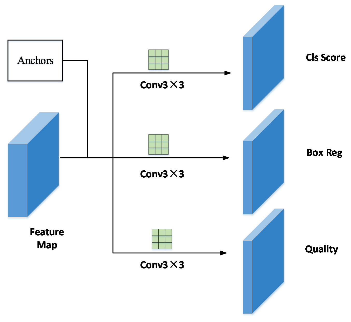
3.2. Feature Enhancement Module

With the generator, we obtained a set of learnable anchor boxes. These anchors not only have the largest IoU score, but also completely surround the ground-truth boxes in the image. We took the anchor shapes as priori information to guide and extract the object features within the scope of the anchors. DCN [31] uses a parallel convolution network to learn the offsets, which makes the rectangular convolution kernel offset at the sampling points of the input feature map, so as to extract the features of the region of interest. As shown in Figure 4, we apply DCN to the feature enhancement module, as:
o f f s e t _ m a p i = conv a n c h o r _ s h a p e i
P i = D C N o f f s e t _ m a p i , P i
where a n c h o r _ s h a p e i is the output of the anchor generator, P i is a feature map from the FPN. We first adopt a 1 × 1 standard convolution to convert the anchor shape of each location into an offset, and obtain an offset map o f f s e t _ m a p i . Then, the original feature map Pi and the offset map o f f s e t _ m a p i are fed into the deformable convolution DCN to extract the features at the offsets and, finally, the enhanced feature map P i is obtained.

3.3. Quality Branch

The detectors usually assign anchors to the ground-truth boxes based on the maximum IoU criterion, which means that an anchor with a higher IoU score is more important. The locations near the bounding box center will produce high-quality anchors in the feature maps, while those away from the center will produce low-quality anchors. However, the loss weights of all predicted anchors are equal when calculating the anchor regression loss, which is unreasonable. To suppress the low-quality anchors, we issued an effective strategy. Specifically, we added a branch to predict the quality of the predicted anchors in parallel with the regression branch.
As shown in Figure 5, the prediction head of the network is composed of three convolution branches to complete the prediction tasks of category, coordinate, and quality, respectively. The decoupling prediction structure greatly reduces the difficulty of classification and regression, and is conducive to parameter optimization. At the same time, in order to improve the reasoning speed, each branch contains only one convolution operation, which significantly reduces the amount of operation. For the input feature map, the prediction head will output three prediction matrices, including Class, Object, and Quality.
Given a ground-truth box g t i = x g t , y g t , w g t , h g t and its corresponding anchor box a n c h o r i = x , y , w , h , the quality target is defined as:
quality g t i , a n c h o r i = g t i a n c h o r i g t i a n c h o r i
At the training stage, the quality is trained with the binary cross entropy (BCE) loss, and the quality target is used as the weight of anchor loss. The final confidence score is computed by multiplying the classification score with the corresponding predicted quality in testing. Therefore, the quality can reduce the scores of the low-quality anchors. By the non-maximum suppression (NMS) [32] process, the most low-quality predicted boxes might be filtered out, improving performance.

3.4. Model Train

3.4.1. Anchor with FPN

To detect objects on multi-level feature maps, we need to predict different sizes of anchors on different levels of feature maps. We use five levels of feature maps defined as P1, P2, P3, P4, and P5, and strides of 8, 16, 32, 64, and 128, respectively. The anchor-based detectors usually design the sizes of anchors according to the level of the feature map. Similarly, we directly limit the anchor shape regression range for each level. More specifically, we set a set of parameters R 0 , R 1 , R 2 , R 3 , R 4 and R 5 , whose values are 0, 64, 128, 256, 512, and , respectively. R i represents the maximum regression distance of map P i . We first calculate shape regression targets w * and h * for each location on all feature maps. Then, if a location satisfies 2 R i 1 m a x w * , h * 2 R i , it is considered as a positive sample and the targets w * and h * will be regress on P i . Otherwise the location is ignored.
X = x × s i + s i 2 ,   Y = y × s i + s i 2
For each location x , y on the feature map P i , we use Equation (8) to map it back to the input image, and the mapped location X , Y is close enough to the center of the receptive field of the location x , y . The location x , y is set as a positive sample if it falls into any ground-truth box and the shape target is obtained by Equation (2). Otherwise the position x , y is a negative sample. When location x , y falls into more than one ground-truth boxes, we choose the box with smaller area.

3.4.2. Loss Function

The proposed Dynamic Anchor is easy to optimize in an end-to-end way, and multi-task loss is used for joint optimization during training. Besides classification loss and regression loss, we also introduce anchor loss and quality loss. The classification loss and regression loss are similar to RetinaNet—we use focal loss and L1 loss, respectively—and both are normalized by the objects inside the batch. We define the training loss function as follows:
L c x , y ,   b x , y , q x , y , a x , y = λ 1 L c l s + λ 2 L r e g + λ 3 N l o c x , y I l x , y * L q l y q x , y , q x , y * + λ 4 N l o c x , y I l x , y * L a n a x , y , a x , y *
L c l s = 1 N α t 1 p t γ l o g p t
L r e g = 1 N x , y b x , y b x , y * 1
L q l y = q x , y * l o g q x , y + 1 q x , y * l o g 1 q x , y
L a n a x , y , a x , y * = 1 a x , y a x , y * a x , y a x , y *
where λ1, λ2, λ3, λ4 0 , 1 are hyper-parameters and used as loss weights. c x , y , b x , y , q x , y and a x , y are the predicted category, regression box, quality, and optimal anchor at (x, y) in the feature map, respectively. “*” represents the label corresponding to the output. N l o c represents the total number of locations in the feature maps used to predict the optimal anchor box. L q l y and L a n are quality loss and anchor loss. In the experiments, we use BCE Loss and IoU Loss [11] as quality loss and anchor loss, and both are averaged by the number of the positive locations. I l x , y * represents an indicator function. If the predicted anchor located in x , y is a positive sample and assigned to a ground-truth box, I l x , y * takes 1. Otherwise, the indicator takes 0. . means “area”, and the union and intersection of the box coordinates are used as shorthand for the boxes themselves. The areas of unions or intersections are computed by min/max of the linear functions of a x , y and a x , y * , which makes the loss sufficiently well-behaved for stochastic gradients.

4. Experiments

4.1. Implementation Details

Dataset: We conducted experiments on the large-scale detection benchmark COCO2017 [20], which contains more than 200,000 images and 80 object categories, including person, bicycle, car, motorbike, airplane, bus, train, truck, boat, traffic light, fire hydrant, bench, and so on. Some of the images are shown in Figure 6. Our models were trained on trainval35k (115k images) split and evaluated on minival split (5k images). Finally, we reported the COCO AP on test-dev split (20k images) by uploading detection results to the evaluation server. The dataset had the characteristics of rich categories, large number, diverse scenes, and large scale range, which made high detection performance very challenging.
Evaluation Metrics: Following the evaluation protocol in MS COCO [8], we used the mean average precision(mAP); average precision of small, medium, and large objects (APS, APM, APL); and average recall of small, medium, and large objects (ARS, ARM, ARL) metrics to evaluate the results. Specifically, mAP was computed by averaging over all 10 intersection-over-union (IoU) thresholds (i.e., in the range 0.50 :   0.95 with the uniform step size 0.05) of all classes. In MS COCO, the small, medium, and large objects refer to these area < 322, 322 < area < 962 and area > 962, respectively. Giga Floating-point Operations Per Second(GFLOPs) was used to measure the calculating consumption.
Training Details: We used MMDetection [33], a deep learning object detection toolbox, to implement Dynamic Anchor. We used Resnet-50 [21] as the backbone network for all experiments, if not otherwise specified. Our network was trained with stochastic gradient descent (SGD) over 2 RXT 3090 GPUs with a total of 8 images per mini-batch for 12 epochs. Weight decay and momentum were set as 0.0001 and 0.9. The initial learning rate was 0.005 and reduced by a factor of 10 at epoch 9 and 11. We resized the input images so that the shorter side was 800 and the longer side less or equal to 1333. We used horizontal flipping as the only data augmentation method, and the weight pre-trained on ImageNet [34] was used to initialize the backbone.

4.2. Ablation Study on COCO

Feature Enhancement with DCN: To verify the effectiveness of DCN [31] in the feature enhancement module, we designed several comparative experiments. We replaced the DCN with a spatial attention module (SAM) [35]. The SAM converts the shape map into a single-channel spatial attention map. The spatial attention map is multiplied by the corresponding feature map from FPN to obtain the output of the feature enhancement module. To be fair, we also did not use DCN nor direct output the original feature map. As shown in Table 1, the DCN does help the improvement in detection performance. Compared with *., DCN increases the APL and ARL by 1.6% and 0.7%, respectively, and achieves 37.0% AP. Generally, large-scale objects contain richer semantic features. With DCN, the detector can predict more accurately and improve the performance of large-scale objects. However, for the small-scale and the medium-scale objects, the shape predictions may not be accurate. Enhancing feature expression with the anchor shapes will damage performance slightly. The work [35] utilizes the SAM in the backbone to pay attention to the regions of the objects, while in the ablation experiment, the application of the SAM in the head impairs performance.
With or Without Quality: As mentioned above, quality was proposed to suppress low-quality anchor boxes produced by locations far from the center of an object. As shown in Table 2, the quality branch can boost AR from 52.9% to 54.7% and AP from 36.7% to 37.2%, improving the detection performance under all metrics. It can be noted that the methods of suppressing low-quality anchors or predictions are applied in many detectors. For example, FCOS proposes “center-ness” to suppress low-quality bounding boxes. Compared with the “center-ness”, quality does not achieve a significant improvement in AP. Reviewing the decoding of bounding boxes in the DA-RetinaNet, we can conclude that predicted anchors and regression boxes determine the predictions of the bounding boxes. In training, the anchor and the box were jointly optimized and dynamically adjusted. The two-time tuning in the shape prediction stage and the regression stage may make it a good prediction for a low-quality anchor. In other words, our method is robust to the different qualities of the predicted anchors.
Center Sampling of the Region: In dynamic anchor, a location is considered a positive sample if it falls into any ground-truth box and its anchor shape target meets the regression range criterion. We obtain considerable positive samples based on the strategy above, making prediction difficult. To reduce the number of the positive samples, we used only the central portion of the ground-truth box as positive samples with the price of one extra hyper-parameter (sampling ratio). As shown in Table 3, with sampling ratio = 2, center sampling improves AP from 37.2% to 37.5%. Meanwhile, center sampling reduces the number of positive anchor boxes, which seriously affects the recall rate of the small-scale objects, decreasing by 1%.

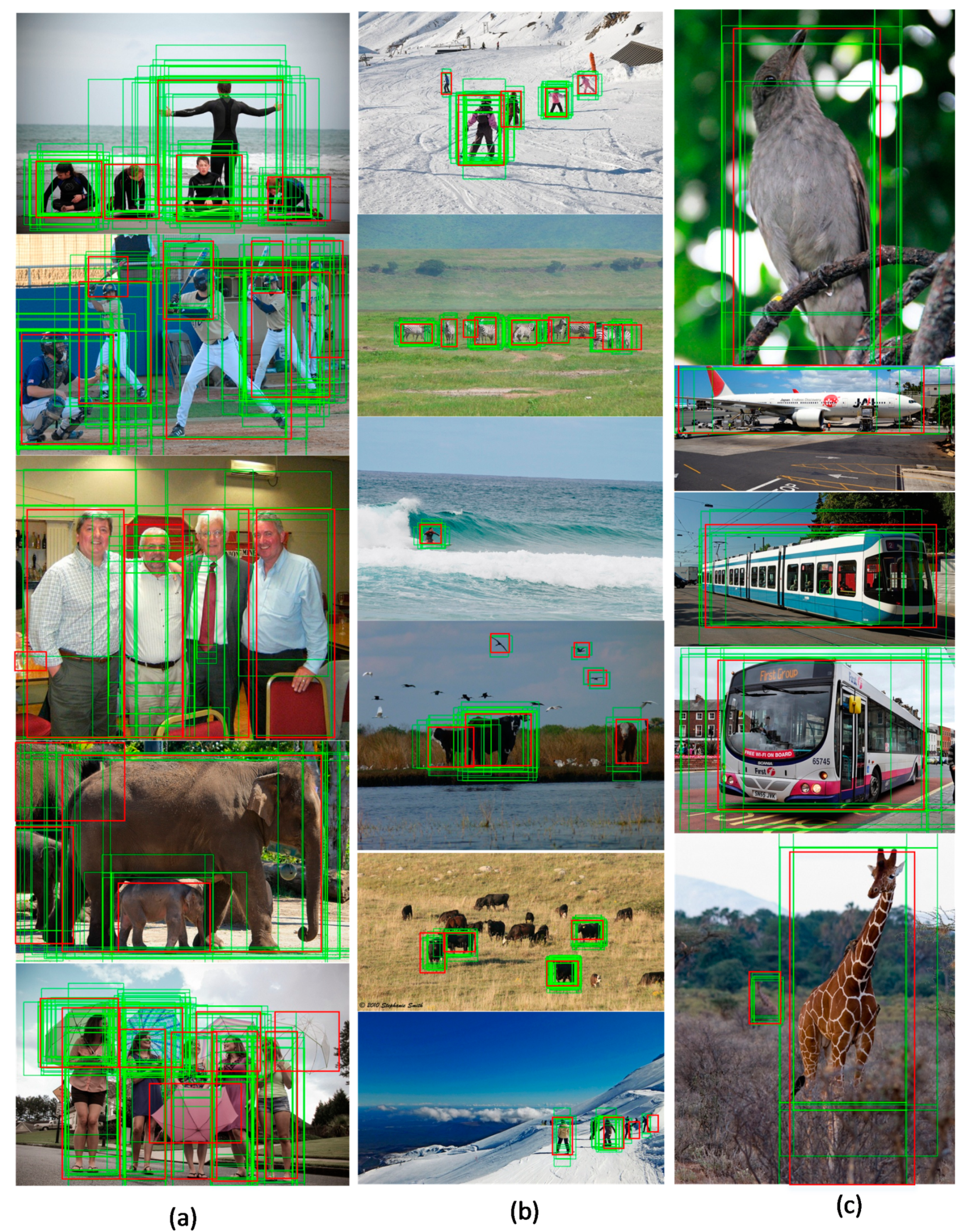
4.3. Visualizing Dynamic Anchor

We visualized the predicted anchors and the ground-truth boxes on the input images. As shown in Figure 7, our method successfully produces multiple anchor boxes for objects, and the predicted anchors have the highest coverages with the corresponding ground-truth boxes. As shown in Figure 7a, for an image containing dense objects, the pre-defined anchor strategy generally improves the recall rate by setting anchor boxes intensively to prevent missing targets. The method proposed in this paper introduces the a priori information of object shape, constructs the corresponding anchor box according to the features of the object, and obtains a large number of candidate boxes with high IoU scores. It can not only maintain a high recall rate, but also reduce the number of anchors on a large scale; In particular, because the size and shape of the pre-defined anchors are fixed, it is unable to handle the objects with too small a size or extreme aspect ratio well, and hyper-parameters needed to be adjusted in the experiment. Our method predicts the appropriate anchors based on the semantic characteristics of each object, which perfectly avoids the above problems and has stronger applicability. As shown in Figure 7b, dynamic anchor generates a large number of anchor boxes for small-scale targets, and the offset distances between these anchor boxes and the ground-truth boxes are very small. These anchor boxes are very suitable for regression. As shown in Figure 7c, the predicted anchor boxes have shapes similar to the ground-truth boxes, and the aspect ratio is very large. To evaluate the quality of all predicted anchors, we treated the predicted anchors as the prediction results. The detection performance reached a considerable 26.5 AP, proving the effectiveness of dynamic anchor.

4.4. Comparison

In this subsection, we show the main results of dynamic anchor. We equipped the previous state-of-art detector RetinaNet with dynamic anchor and used ResNet-50 and ResNet-101 as the backbones. To verify the efficiency of our method, we also compared dynamic anchor with guided anchoring. As presented in Table 4, dynamic anchor with ResNet-50 and Res-Net101 as the backbone networks achieved an AP of 38.0% and 40.0% on COCO test-dev 2017, respectively, which outperformed RetinaNet and GA-RetinaNet. Compared to the baseline and the counterpart, our model achieved 2.4% and 1.2% AP improvement, and the AP metric of DA-RetinaNet outperformed the other detectors on all size of objects. DA-RetinaNet also achieved a stable improvement for detection with Res-Net101, while the APS metric was slightly lower than RetinaNet (21.5% vs. 21.8%). The improvement of our model comes from medium and large object detection, which is the strength of dynamic anchor, as dynamic anchor can generate anchors with the theoretical maximum IoU scores.
Based on semantic features, Guided Anchor predicts the locations where the center of objects of interest are likely to exist, as well as the scales and aspect ratios at different locations. In training, Guided Anchor uses IoU scores of the pre-defined anchors and the ground-truth boxes to determine the positive sample points in the feature maps, and also sets an initial reference box for each position to regress the anchor of the object. Guided Anchor employs the pre-defined anchors and the initial reference boxes to predict anchors; its performance is severely affected by these boxes, which does not avoid the defect of the pre-defined anchor. Guided Anchor does not break away from the frame of the manual anchor in the anchor-based detectors. However, our dynamic anchor does not introduce any pre-defined boxes, and instead achieves better detection performance.
Moreover, compared with RetinaNet and GA-RetinaNet, the DA-RetinaNet shares the heads between different feature levels and predicts only one anchor box at each point on the feature map, making the detector more parameter-efficient. In the GFLOPs metric, our method with ResNet-50 only reached 141.79, which is 29.6% and 28.1% lower than RetinaNet and GA-RetinaNet, respectively. Similar results were obtained on ResNet-101. To sum up, sufficient experiments have proved that our method is not only superior to other methods in detection performance, but also has significant advantages in reasoning speed.

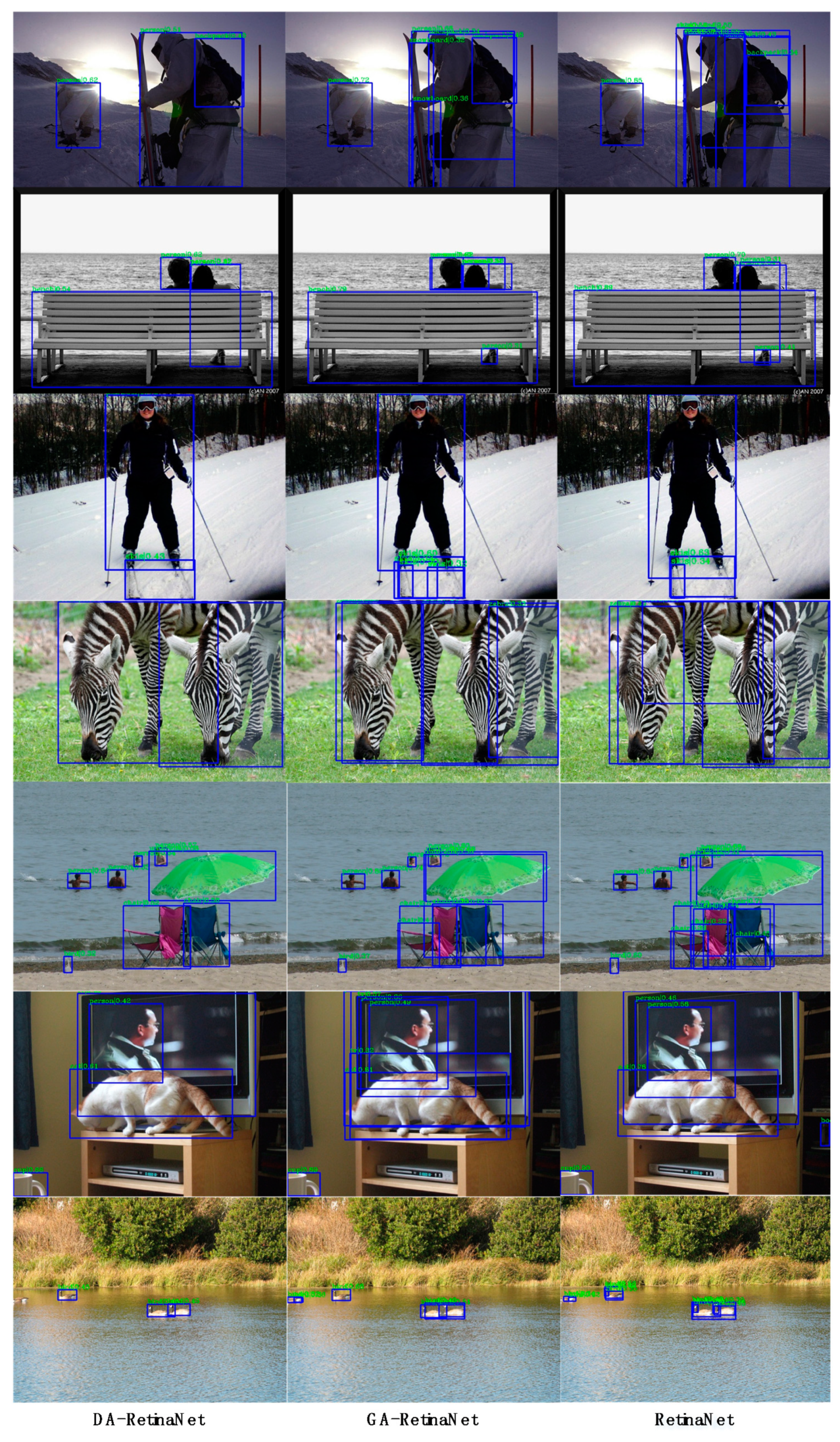
4.5. Visualization Results

The first and fourth row in Figure 8 show a common difficulty in the COCO dataset. There are overlaps between a large number of objects, which are difficult to distinguish, such as pedestrians with backpacks and parallel zebras. It can be seen that RetinaNet and GA-RetinaNet produce numerous redundant and overlapping detection boxes, and these boxes originate from a large quantity of pre-defined anchor boxes with poor quality, which are difficult to remove with post-processing. However, our method produces concise and accurate detection boxes by virtue of an efficient anchor prediction mechanism, avoiding invalid results.
In the second row in Figure 8, the person is seriously blocked by the bench, which requires the model to establish a long-distance information dependence between the head and feet. Both RetinaNet and GA-RetinaNet recognize the head and foot as two objects. In the feature enhancement module, our model extracts the features of anchor regions and integrates the semantic information of the head and feet to obtain a complete detection box. The other rows are similar and our algorithm always outperforms other methods in detecting overlapping targets.

5. Conclusions

In this work, we analyzed the shortcomings of the pre-defined anchor strategy in the field of object detection and proposed the dynamic anchor to generate anchor boxes by semantic features. The dynamic anchor does not rely on any pre-defined boxes, avoiding hyper-parameters related to anchor boxes entirely. To obtain high-quality anchors, we constructed the optimization constraint equation and solved it to obtain the optimal solution. The proposed anchor generator was used to predict the optimal anchor on the feature map. To suppress the low-quality anchor, the quality branch was designed to predict the IoU scores of the anchor box, and the scores served as the corresponding loss weight, which improved the performance significantly.
We implemented dynamic anchor with RetinaNet. With ResNet-50 and ResNet-101 as a backbone, dynamic anchor made considerable performance improvements on RetinaNet. Our method is also superior to the peer method, Guided Anchor. Dynamic anchor can be used to replace the manual anchor strategy for anchor-based detectors.

Author Contributions

X.L. proposed the frameworks and conducted the experiments; H.-X.C. provided suggestions and reviewed the manuscript; B.-Y.L. wrote the manuscript together with X.L. and reviewed the manuscript. All authors have read and agreed to the published version of the manuscript.

Funding

This research was funded by Sichuan Major Science and Technology Special Project grant number 2018GZDZX0017.

Institutional Review Board Statement

Not applicable.

Informed Consent Statement

Not applicable.

Data Availability Statement

All the data used in this paper is from COCO 2019 Object Detection Task, which can be found in https://cocodataset.org/#detection-2019 (accessed on 21 February 2022).

Conflicts of Interest

The authors declare no conflict of interest.

References

  1. Zou, Z.; Shi, Z.; Guo, Y.; Ye, J. Object detection in 20 years: A survey. arXiv 2019, arXiv:1905.05055. [Google Scholar]
  2. Huang, Z.; Chen, H.; Zhou, T.; Yang, Y.; Liu, B. Multi-level cross-modal interaction network for RGB-D salient object detection. Neurocomputing 2021, 452, 200–211. [Google Scholar] [CrossRef]
  3. Liu, B.; Chen, H.; Huang, Z.; Liu, X.; Yang, Y. ZoomInNet: A Novel Small Object Detector in Drone Images with Cross-Scale Knowledge Distillation. Remote Sens. 2021, 13, 1198. [Google Scholar] [CrossRef]
  4. Ren, S.; He, K.; Girshick, R.; Sun, J. Faster R-CNN: Towards real-time object detection with region proposal networks. IEEE Trans. Pattern Anal. Mach. Intell. 2017, 39, 1137–1149. [Google Scholar] [CrossRef] [Green Version]
  5. Redmon, J.; Farhadi, A. Yolo9000: Better, Faster, Stronger. In Proceedings of the IEEE Conference on Computer Vision and Pattern Recognition, Honolulu, HI, USA, 21–26 July 2017; IEEE: Piscataway, NJ, USA, 2017; pp. 7263–7271. [Google Scholar]
  6. Redmon, J.; Farhadi, A. Yolov3: An incremental improvement. arXiv 2018, arXiv:1804.02767. [Google Scholar]
  7. Liu, W.; Anguelov, D.; Erhan, D.; Szegedy, C.; Reed, S.; Fu, C.; Berg, A. Ssd: Single Shot Multibox Detector. In Proceedings of the European Conference on Computer Vision, Amsterdam, The Netherlands, 11–14 October 2016; Springer: Berlin/Heidelberg, Germany, 2016; pp. 21–37. [Google Scholar]
  8. Lin, T.Y.; Goyal, P.; Girshick, R.; He, K.; Dollár, P. Focal Loss for Dense Object Detection. In Proceedings of the IEEE International Conference on Computer Vision, Venice, Italy, 22–29 October 2017; IEEE: Piscataway, NJ, USA, 2017; pp. 2980–2988. [Google Scholar]
  9. Redmon, J.; Divvala, S.; Girshick, R.; Farhadi, A. You Only Look Once: Unified, Real-Time Object Detection. In Proceedings of the IEEE Conference on Computer Vision and Pattern Recognition, Las Vegas, NV, USA, June 26–July 1 2016; IEEE: Piscataway, NJ, USA, 2016; pp. 779–788. [Google Scholar]
  10. Huang, L.; Yang, Y.; Deng, Y.; Yu, Y. Densebox: Unifying landmark localization with end to end object detection. arXiv 2015, arXiv:1509.04874. [Google Scholar]
  11. Yu, J.; Jiang, Y.; Wang, Z.; Cao, Z.; Huang, T. Unitbox: An Advanced Object Detection Network. In Proceedings of the 24th ACM International Conference on Multimedia, Amsterdam, The Netherlands, 15–19 October 2016; ACM: New York, NY, USA, 2016; pp. 516–520. [Google Scholar]
  12. Law, H.; Deng, J. Cornernet: Detecting Objects as Paired Keypoints. In Proceedings of the European Conference on Computer Vision, Munich, Germany, 8–14 September 2018; Springer: Berlin/Heidelberg, Germany, 2018; pp. 734–750. [Google Scholar]
  13. Zhu, C.; He, Y.; Savvides, M. Feature Selective Anchor-Free Module for Single-Shot Object Detection. In Proceedings of the IEEE/CVF Conference on Computer Vision and Pattern Recognition, Long Beach, CA, USA, 15–20 June 2019; IEEE: Piscataway, NJ, USA, 2019; pp. 840–849. [Google Scholar]
  14. Duan, K.; Bai, S.; Xie, L.; Qi, H.; Huang, Q.; Tian, Q. Centernet: Keypoint Triplets for Object Detection. In Proceedings of the IEEE/CVF International Conference on Computer Vision, Seoul, Korea, 27–28 October 2019; IEEE: Piscataway, NJ, USA, 2019; pp. 6569–6578. [Google Scholar]
  15. Kong, T.; Sun, F.; Liu, H.; Jiang, Y.; Li, L.; Shi, J. Foveabox: Beyound Anchor-Based Object Detection. IEEE Trans. Image Process. 2020, 29, 7389–7398. [Google Scholar] [CrossRef]
  16. Liu, L.; Ouyang, W.; Wang, X.; Fieguth, P.; Chen, J.; Liu, X.; Pietikäinen, M. Deep learning for generic object detection: A survey. Int. J. Comput. Vis. 2020, 128, 261–318. [Google Scholar] [CrossRef] [Green Version]
  17. Zhang, S.; Chi, C.; Yao, Y.; Lei, Z.; Li, S.Z. Bridging the Gap between Anchor-Based and Anchor-Free Detection via Adaptive Training Sample Selection. In Proceedings of the IEEE/CVF Conference on Computer Vision and Pattern Recognition, Seattle, WA, USA, 16–18 June 2020; IEEE: Piscataway, NJ, USA, 2020; pp. 9759–9768. [Google Scholar]
  18. Tian, Z.; Shen, C.; Chen, H.; He, T. Fcos: Fully Convolutional One-Stage Object Detection. In Proceedings of the IEEE/CVF International Conference on Computer Vision, Seoul, Korea, 27 October–2 November 2019; IEEE: Piscataway, NJ, USA, 2019; pp. 9627–9636. [Google Scholar]
  19. Lin, T.Y.; Dollár, P.; Girshick, R.; He, K.; Hariharan, B.; Belongie, S. Feature Pyramid Networks for Object Detection. In Proceedings of the IEEE Conference on Computer Vision and Pattern Recognition, Honolulu, HI, USA, 21–26 July 2017; IEEE: Piscataway, NJ, USA, 2017; pp. 2117–2125. [Google Scholar]
  20. Lin, T.Y.; Maire, M.; Belongie, S.; Hays, J.; Perona, P.; Ramanan, D.; Dollár, P.; Zitnick, C.L. Microsoft Coco: Common Objects in Context. In Proceedings of the European Conference on Computer Vision, Zurich, Switzerland, 6–12 September 2014; Springer: Berlin/Heidelberg, Germany, 2014; pp. 740–755. [Google Scholar]
  21. He, K.; Zhang, X.; Ren, S.; Sun, J. Deep Residual Learning for Image Recognition. In Proceedings of the IEEE Conference on Computer Vision and Pattern Recognition, Las Vegas, NV, USA, 27–30 June 2016; IEEE: Piscataway, NJ, USA, 2016; pp. 770–778. [Google Scholar]
  22. Wang, J.; Chen, K.; Yang, S.; Loy, C.C.; Lin, D. Region Proposal by Guided Anchoring. In Proceedings of the IEEE/CVF Conference on Computer Vision and Pattern Recognition, Long Beach, CA, USA, 15–20 June 2019; IEEE: Piscataway, NJ, USA, 2019; pp. 2965–2974. [Google Scholar]
  23. Zhao, Q.; Sheng, T.; Wang, Y.; Tang, Z.; Chen, Y.; Cai, L.; Ling, H. M2det: A Single-Shot Object Detector Based on Multi-Level Feature Pyramid Network. In Proceedings of the AAAI Conference on Artificial Intelligence, Honolulu, HI, USA, January 27–1 February 2019; AAAI Press: Palo Alto, CA, USA, 2019; pp. 9259–9266. [Google Scholar]
  24. Zhang, S.; Wen, L.; Bian, X.; Lei, Z.; Li, S.Z. Single-Shot Refinement Neural Network for Object Detection. In Proceedings of the IEEE Conference on Computer Vision and Pattern Recognition, Salt Lake City, UT, USA, 18–22 June 2018; IEEE: Piscataway, NJ, USA, 2018; pp. 4203–4212. [Google Scholar]
  25. Fu, C.Y.; Liu, W.; Ranga, A.; Tyagi, A.; Berg, A.C. Dssd: Deconvolutional single shot detector. arXiv 2017, arXiv:1701.06659. [Google Scholar]
  26. Dai, J.; Li, Y.; He, K.; Sun, J. R-fcn: Object Detection via Region-Based Fully Convolutional Networks. In Advances in Neural Information Processing Systems, Proceedings of the 2016 Conference on Neural Information Processing Systems, Barcelona, Spain, 5–10 December 2016; NIPS: Los Angeles, CA, USA, 2016; p. 3. [Google Scholar]
  27. Cai, Z.; Vasconcelos, N. Cascade r-cnn: Delving into High Quality Object Detection. In Proceedings of the IEEE Conference on Computer Vision and Pattern Recognition, Salt Lake City, UT, USA, 18–22 June 2018; IEEE: Piscataway, NJ, USA, 2018; pp. 6154–6162. [Google Scholar]
  28. Zhong, Q.; Li, C.; Zhang, Y.; Xie, D.; Yang, S.; Pu, S. Cascade region proposal and global context for deep object detection. Neurocomputing 2020, 395, 170–177. [Google Scholar] [CrossRef] [Green Version]
  29. Kim, K.; Lee, H.S. Probabilistic Anchor Assignment with Iou Prediction for Object Detection. In Proceedings of the European Conference on Computer Vision, Glasgow, UK, 23–28 August 2020; Springer: Berlin/Heidelberg, Germany, 2020; pp. 355–371. [Google Scholar]
  30. Yang, T.; Zhang, X.; Li, Z.; Zhang, W.; Sun, J. Metaanchor: Learning to Detect Objects with Customized Anchors. Advances in Neural Information Processing Systems, Montreal, QC, Canada, 2–8 December 2018; NIPS: Los Angeles, CA, USA, 2018; p. 31. [Google Scholar]
  31. Dai, J.; Qi, H.; Xiong, Y.; Li, Y.; Zhang, G.; Hu, H.; Wei, Y. Deformable Convolutional Networks. In Proceedings of the IEEE International Conference on Computer Vision, Venice, Italy, 22–29 October 2017; IEEE: Piscataway, NJ, USA, 2017; pp. 764–773. [Google Scholar]
  32. Neubeck, A.; Van Gool, L. Efficient Non-Maximum Suppression. In Proceedings of the 18th International Conference on Pattern Recognition, Hong Kong, China, 20–24 August 2006; IEEE: Piscataway, NJ, USA, 2006; pp. 850–855. [Google Scholar]
  33. Chen, K.; Wang, J.; Pang, J.; Cao, Y.; Xiong, Y.; Li, X.; Lin, D. MMDetection: Open mmlab detection toolbox and benchmark. arXiv 2019, arXiv:1906.07155. [Google Scholar]
  34. Krizhevsky, A.; Sutskever, I.; Hinton, G.E. Imagenet classification with deep convolutional neural networks. Adv. Neural Inf. Processing Syst. 2012, 25, 1097–1105. [Google Scholar] [CrossRef]
  35. Woo, S.; Park, J.; Lee, J.Y.; Kweon, I.S. Cbam: Convolutional Block Attention Module. In Proceedings of the European Conference on Computer Vision, Munich, Germany, 8–14 September 2018; Springer: Berlin/Heidelberg, Germany, 2018; pp. 3–19. [Google Scholar]
Figure 1. This is the schematic diagram of a set of pre-defined anchor boxes. There are nine anchors with different scales and aspect ratios. The red box represents the anchors and the blue box represents the ground-truth box.
Applsci 12 04897 g001
Figure 2. Illustration of our framework. In dynamic anchor, we employ the anchor generator, a fully convolutional branch to predict the best anchor shape for each location in the feature maps. Then the feature enhancement module is used to enhance feature expression. Finally, we propose the quality branch to suppress low-quality anchors.
Applsci 12 04897 g002
Figure 3. (a) The red box and the black box represent the ground-truth box x g t , y g t , w g t , h g t and the corresponding pre-defined anchor x , y , w , h , respectively. ( x g t , y g t ) is the coordinate of the center point of the ground-truth box. w g t and h g t represent the width and height of the of the ground-truth box, respectively. l, t, r and b are the distances from the location x , y to the four sides of ground-truth box. The width w g t and height h g t are calculated by w g t = l + r and h g t = t + b ; (b) The yellow box x , y , 2 r , 2 b represents the best anchor box of box x g t , y g t , w g t , h g t .
Applsci 12 04897 g003
Figure 4. Illustration of the feature enhancement module.
Applsci 12 04897 g004
Figure 5. The structure of the head. The decoupling prediction structure is composed of three convolution branches.
Applsci 12 04897 g005
Figure 6. Some images in COCO2017 datasets. The dataset has the characteristics of rich categories, large number, diverse scenes, and large scale range, which makes high detection performance very challenging.
Applsci 12 04897 g006
Figure 7. Visualization results of predicted anchors (green boxes) and ground-truth boxes (red boxes) in DA-RetinaNet. (a) Input images with dense objects; (b) input images with small-scale objects; (c) input images with extremely wide objects.
Applsci 12 04897 g007
Figure 8. Comparison of the detection results of the DA-RetinaNet, GA-RetinaNet and RetinaNet.
Applsci 12 04897 g008
Table 1. The effects of different modules in our Feature Enhancement. *., SAM, and DCN denote without operator, spatial attention mechanism, or deformable convolution, respectively. Bold font indicates the best results.
*.SAMDCNAPAP50AP75APSAPMAPLARSARMARL
36.753.939.819.942.148.632.259.570.6
36.453.439.219.441.847.832.058.969.6
37.053.940.219.141.650.231.959.071.3
Table 2. Ablation study for quality branch on the MS COCO minival set. “None” denote that no “quality” is used. “Quality” is that using quality predicted from the quality branch. Bold font indicates the best results.
APAP50AP75AR100AR300AR1000
None36.754.339.852.952.952.9
Quality37.254.640.254.754.754.7
Table 3. The results of different center sampling ratio on the MS COCO minival set. Bold font indicates the best results.
Sampling RatioAPAP50AP75APSAPMAPLARSARMARL
None37.254.440.220.241.650.433.559.070.6
137.254.640.220.542.349.532.659.971.4
1.537.354.840.220.142.149.633.259.670.6
237.554.940.520.142.450.732.559.370.8
Table 4. The compared results on MS COCO 2017 test-dev. We used AP, AP50, AP75, APS, APM, APL to evaluate the performance of the three models and counted the floating-point computation (GFLOPs) of all models.
MethodBackboneAPAP50AP75APSAPMAPLGFLOPs
RetinaNetResNet-5035.955.438.819.438.946.5201.53
GA-RetinaNetResNet-5037.156.940.020.140.148.0197.43
DA-RetinaNet(ours)ResNet-5038.055.541.220.141.848.5141.79
RetinaNetResNet-10139.159.142.321.842.750.2277.6
GA-RetinaNetResNet-10138.458.541.321.041.149.7273.5
DA-RetinaNet(ours)ResNet-10140.057.943.521.544.151.2217.86
Publisher’s Note: MDPI stays neutral with regard to jurisdictional claims in published maps and institutional affiliations.

