Size and Shape Optimization of a Guyed Mast Structure under Wind, Ice and Seismic Loading

Abstract

This paper discusses the size and shape optimization of a guyed radio mast for radiocommunications. The considered structure represents a widely industrial solution due to the recent spread of 5G and 6G mobile networks. The guyed radio mast was modeled with the finite element software SAP2000 and optimized through a genetic optimization algorithm (GA). The optimization exploits the open application programming interfaces (OAPI) SAP2000-Matlab. Static and dynamic analyses were carried out to provide realistic design scenarios of the mast structure. The authors considered the action of wind, ice, and seismic loads as variable loads. A parametric study on the most critical design variables includes several optimization scenarios to minimize the structure’s total self-weight by varying the most relevant parameters selected by a preliminary sensitivity analysis. In conclusion, final design considerations are discussed by highlighting the best optimization scenario in terms of the objective function and the number of parameters involved in the analysis.

1. Introduction

Guyed masts are extensively used in the telecommunications industry, and the size, shape, and topology optimization can significantly benefit their transportation and installation. The main loads acting on guyed mast structures arise from wind [1,2], earthquakes [3,4,5,6], sudden rupture of guys [7], galloping of guys [8], and sudden ice shedding from ice-laden guy wires [9].

Their optimization must fulfil several requirements under ultimate and service limit states [10]. Specifically, service limit states are crucial for guyed mast structures due to high-amplitude oscillations caused by their high deformability. In some cases, these vibrations have led to a signal loss caused by excessive displacement and rotation of the antennas and, in other cases, have resulted in permanent deformation or failure. Therefore, size optimization of the guyed mast structure represents a challenging task since the increment of the performance ratio of the materials should be counterbalanced by an adequate lateral stiffness to reduce high-vibration drawbacks [11].

Saxena [12] reported several happenings where heavy icing combined with moderate wind resulted in severe misalignment of towers and complete failure. Novak et al. [13] showed that ice accumulation on some parts of the guy wires and moderate winds could lead to the guy galloping, resulting in unacceptable stress levels throughout the structure. The main topics investigated in the field of guyed structures can be summarized as follows:

• Structural design. Several researchers investigated the dynamic response of guyed mast structures through experimental tests and numerical modeling to derive design approaches and recommendations [14,15,16]. In particular, there are studies dealing with the dynamic identification and accurate estimate of the wind loads [17,18,19,20,21].
• Nonlinear dynamics. The proneness to global and local instabilities challenged several scholars to estimate and predict the nonlinear behaviour of guyed masts [22,23,24,25,26].
• Structural optimization. The need for guyed structures that are easy to install and transport challenged several scholars to optimize their shape in order to reduce the structural mass without reducing the lateral stiffness and prevent instability phenomena [27].
• Structural control. There are some attempts of control methods to reduce vibrations in mast-like structures [28,29,30]. Among others, Blachowski [31] proposed the use of a hydraulic actuator to control cable forces in guyed masts using Kalman filtering.

This paper tackles the size and shape optimization of guyed mast structures. A video of the considered structure is available in Supplementary Material. Since the first attempts by Bell and Brown [32], many engineers attempted to optimize guyed masts under wind loads using deterministic global optimization algorithms. However, as pointed out by [27], this approach leads to local optimum points, since each design variable was considered separately. Thornton et al. [33] and Uys et al. [34] proposed general procedures for optimizing steel towers under dynamic loads. To the author’s knowledge, Venanzi and Materazzi [35] were the first to implement a multi-objective optimization method for guyed mast structures under wind loads using the stochastic simulated annealing algorithm for size optimization. The objective function implemented by [35] included the sum of the squares of the nodal displacements and the in-plan width of the structure. Zhang and Li [36] attempted to achieve both shape and size optimization in a two-step procedure using the ant colony algorithm (ACA). Cucuzza et al. [37] proposed an alternative approach in which the multi-objective optimization problem has been reduced to a single-objective problem through suitable parameters. Luh and Lin [38] were challenged in achieving the topology, size, and shape optimization of guyed masts using a modification of the binary particle swarm optimization (PSO) and the attractive and repulsive particle swarm optimization.

This paper discusses the size optimization of guyed masts using a genetic algorithm (GA) by considering different design scenarios (e.g., Cucuzza et al. [37] and Manuello et al. [39]). Kaveh and Talatahari [40] noticed that the particle swarm optimization (PSO) is more effective than ACA and the harmony search scheme for optimizing truss structures. However, Deng et al. [41] and Guo and Li [42] were successful in optimizing tapered masts and transmission towers using modifications of genetic algorithms (GA). Moreover, Belevivcius et al. [27] attempted the topology-sizing optimization problem of the guyed mast as a single-level single-objective global optimization problem using GAs.

Therefore, given the numerous successful solutions of guyed masts using GAs, the authors chose to investigate the size optimization of a guyed mast structure using GAs. Following [35], this paper focuses on the size optimization by considering eight possible design scenarios. The purpose of the present paper is two-fold. Firstly, this work aims at achieving a size optimization on a real application case adopting structural verification according to Eurocode 3. During the load evaluation phase, detailed analyses have been conducted, including wind, ice, and seismic actions and the verifications against instabilities. Secondly, the computational intelligence procedure adopted by the authors allowed the investigation of several scenarios simultaneously. As a result, the parameters that mainly affected the design process have been detected to provide preliminary indications to engineers in the practical design of similar structural typologies. Furthermore, the considered case study may represent a benchmark case for validating the reliability and accuracy of alternative numerical approaches. Therefore, the paper is organized as follows. After the case study description and the FE model, the authors introduce the first numerical results and the outcomes of the size and shape optimization.

2. Case Study

The considered structure is a guyed radio mast. It is a thin, slender, vertical structure sustained by tension cables fixed to the ground and typically arranged at 120° between each other.

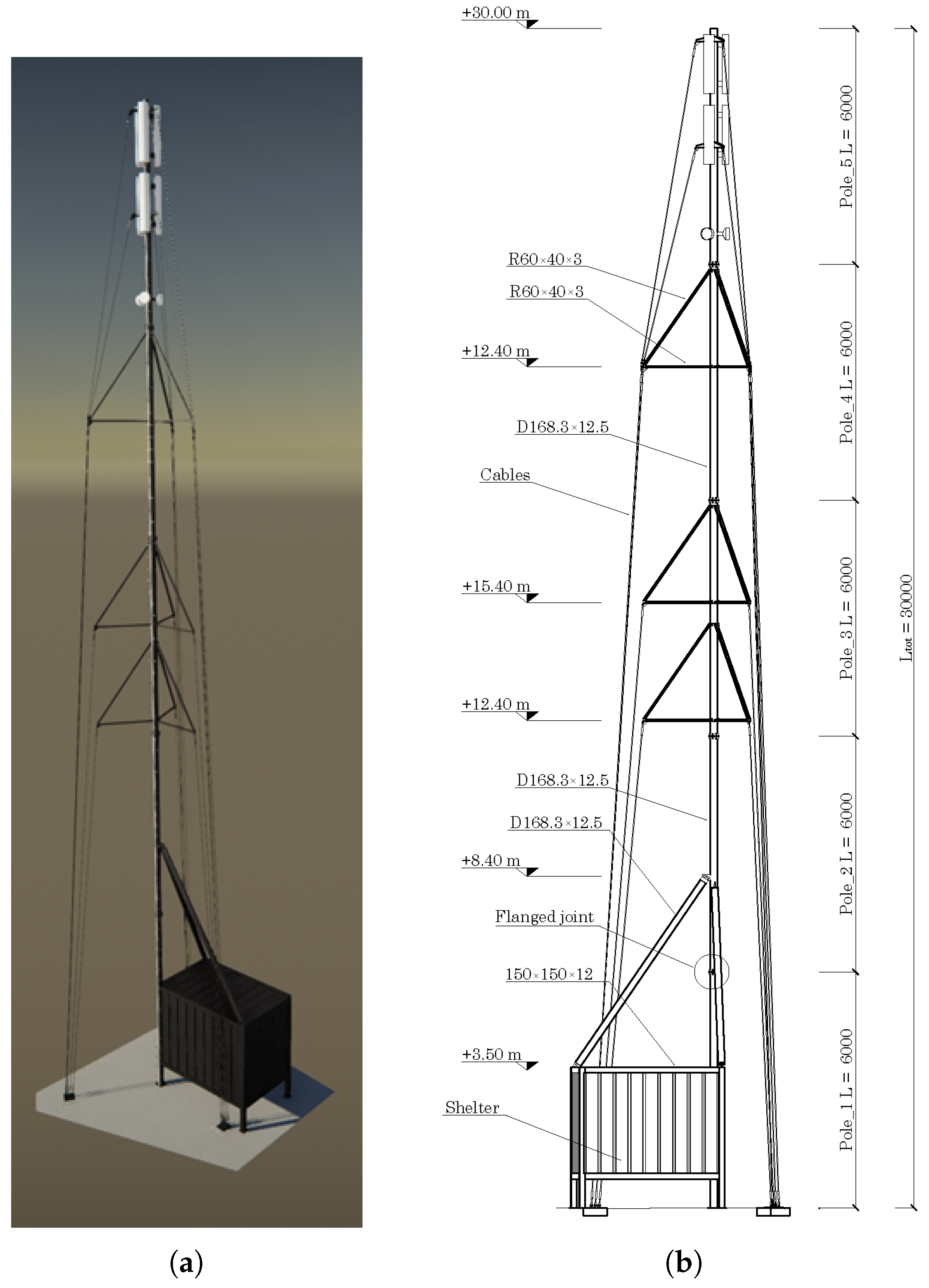
The main body is a single central column made of tube profiles or truss systems when a high elevation must be reached, see Figure 1. More than one set of cables is placed at different elevations to prevent instability phenomena. Guyed towers are usually built for meteorological purposes or to support radio antennas, such as the one considered in this research. In particular, this structure can be used for a limited time during an event or maintenance of primary transmission towers. Therefore, it is also called a temporary base transceiver station (BTS), typically adopted to supply the immediate service. Sporting events, concerts, motor racing, military camps, and emergency events are typical examples of temporary BTS applications. The BTS is usually mounted on a moveable platform called the shelter.

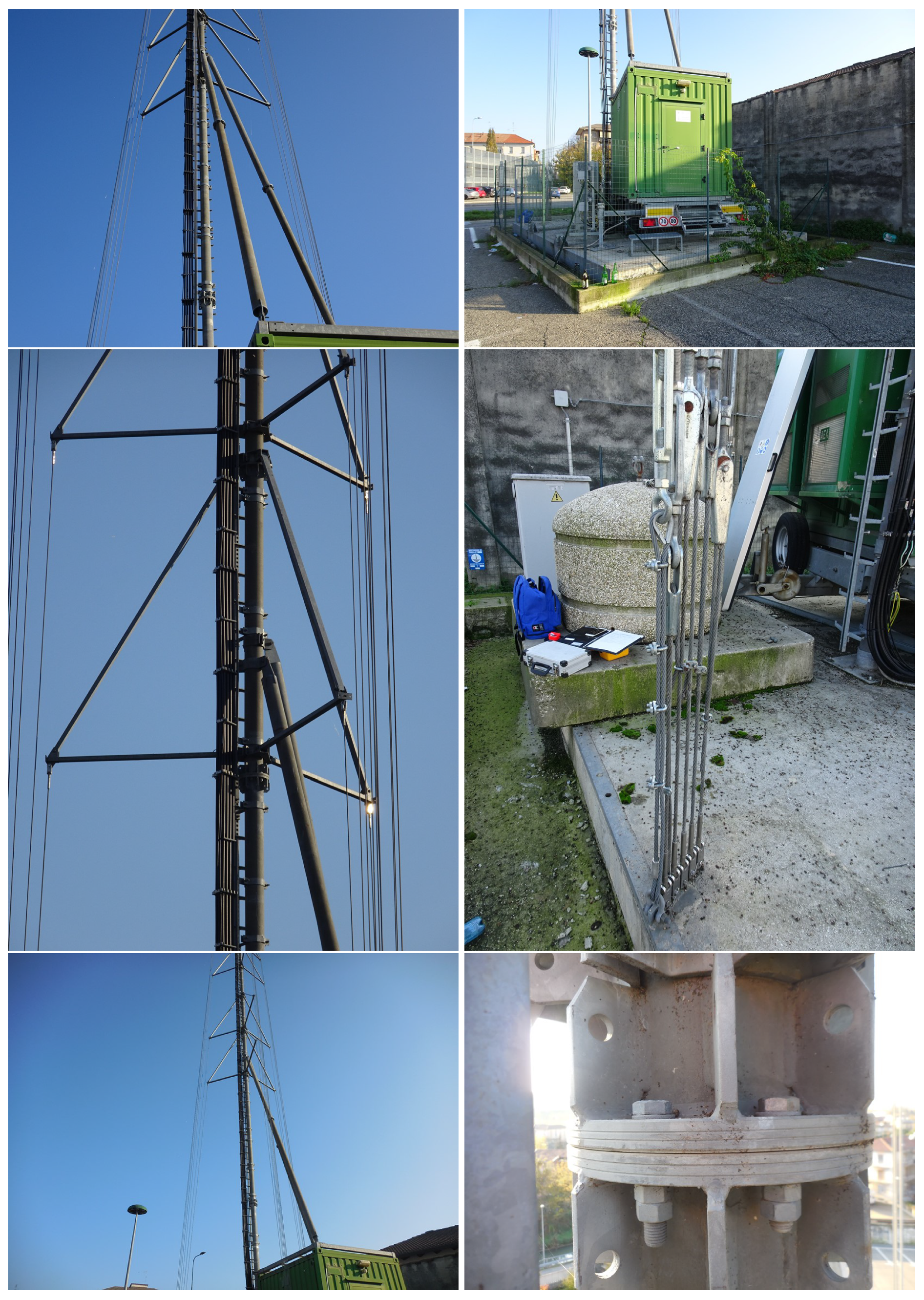
The considered structure is located in Bassano Del Grappa, in the north of Italy, at a 129 m elevation from the sea level. The surrounding area is low-urbanized, with no relevant obstacles to the wind loads. The total height of the mast is 30.00 m. It is sustained by a central pole where 21 cables are fixed, see Figure 2. Other structural elements with rectangular cross-sections are used to create truss systems connecting cables and the central pole.

The central pole consists of five circular hollow steel profiles with flanged joints and 6 m in length. All connections are bolted, as well as those connecting the cables to the pole. The shelter is a steel box devoted to partially sustaining the structure and hosting electronic equipment. It is usually mounted on a moveable platform.

3. Load Analysis

This section details the loads acting on the structures, from the dead to the variable loads. According to the Italian Standard Regulation NTC2018, the load combinations of the actions have been evaluated at the ultimate limit state (ULS) and, for seismic conditions, at the life safety (LS) limit state. In Appendix A,

Table A4. Load combination.

Load Combination
ULS Max${}_1$	$1.3·G_1+1.5·G_2+1.5·Win{d}_1+1.5·0.5·Ic{e}_1+1.5·0·Q_M$
ULS Max1${}_2$	$1.3·G_1+1.5·G_2+1.5·Q_M+1.5·0.6·Win{d}_1+1.5·0.2·Ic{e}_1$
ULS Min${}_1$	$1·G_1+0.8·G_2+1.5·Win{d}_1+1.5·0.5·Ic{e}_1+1.5·0·Q_M$
Quake${}_1$	$E+G_1+G_2+0·Win{d}_1+0·Ic{e}_1+0·Q_M$
ULS Max${}_2$	$1.3·G_1+1.5·G_2+1.5·Win{d}_2+1.5·0.5·Ic{e}_2+1.5·0·Q_M$
ULS Max2${}_1$	$1.3·G_1+1.5·G_2+1.5·Q_M+1.5·0.6·Win{d}_2+1.5·0.2·Ic{e}_2$
ULS Min${}_1$	$1·G_1+0.8·G_2+1.5·Win{d}_2+1.5·0.5·Ic{e}_2+1.5·0·Q_M$
Quake${}_2$	$E+G_1+G_2+0.8·Win{d}_2+1.5·Ic{e}_2+1.5·Q_M$

illustrates the most critical combinations for both static and dynamic configurations. Partial safety factors $\gamma$ and combination coefficients $\psi$ were adopted in order to consider maximization (positive sign) or minimization (negative sign) of effects both for vertical and horizontal actions.

3.1. Dead Loads

The structure is made of steel S355, whose mechanical stress-strain behaviour is depicted in Figure 3, and the characteristics are listed here: $f_{us}=$ 510 MPa, $f_{ys}=$ 355 MPa, $E_s$ = 210,000 MPa, which are the ultimate and yielding stresses and Young’s modulus, respectively.

The cables are made of galvanized steel consisting of 6 strands (216 wires) with an independent metal core (49 wires). The main characteristics are illustrated in

Table 1. Technical specifications of the steel ropes.

Steel Ropes (Cables)
Model			6 × 36WS + IWRC/265 wires
Construction pattern			6 × (14 + (7 + 7) + 7 + 1) + (7 × 7)
Winding direction			right cross
Material			galvanized steel
Resistance			1170 N/mm${}^2$–180 kg/mm${}^2$
Cable diameter	Weight	Area	Wire diameter	Load to failure
[mm]	[kg/m]	[mm${}^2$]	[mm]	[kN]
16	1.36	173.25	0.91	161
18	1.67	212.74	1.03	204
20	2.02	257.32	1.14	252
22	2.41	307.01	1.26	305

.

The structure investigated consists of a few types of elements, as indicated in

Table 2. Computation of the dead loads.

Computation of Dead Loads
Profile [mm]		w [kg/m]	Length [m]	n°	Wtot [kg]
Circular	D168.3 × 12.5	48	6	5	1440
	D168.3 × 12.5	48	5.65	2	543
Rectangular	60 × 40 × 3	4.35	3.16	9	124
	60 × 40 × 3	4.35	1.8	9	71
	100 × 40 × 3	6.13	0.45	6	17
Rope	D16	1.3667	12.45	3	51
	D16	1.3667	15.44	3	63
	D16	1.3667	24.43	9	300
	D16	1.3667	5.76	3	24
	D16	1.3667	8.46	3	35
				2651 Kg

. Dead loads are calculated from the weight per unit length of each member.

The non-structural dead loads originate from the wiring weight and the steel ladder for inspection and maintenance. This load results in 0.3 kN/m. Antennas and parabolas represent the weight of the equipment. Two groups of three antennas are located at 26.00 and 29.25 m in height, with a 120° in mutual spacing. The first one is the model AOC4518R7v06 produced by Huawei^®. The second one is the model 6888670N manufactured by Amphenol^®. Finally, there are three parabolas located at 23.15 m height, spaced 120° apart from each other, 30 cm in diameter.

Table 3. Weight of equipment, H, W, and D stand for height, width, and depth.

Typology	Model	No	Elevation [m]	H × W × D [mm]	Self-Weight [kg]	Clamps [kg]	Total [kg]
Antenna	AOC4518R7v06	3	29.25	1509 × 469 × 206	39.3	2 × 5.8	153
Antenna	6888670N	3	26	1997 × 305 × 163	32	2 × 3.9	119
Parabola	n.d	3	23.15	Diameter = 300	15	2.2	51.6

and

Table 4. Non-structural dead loads.

Item	qk [kN/m]	Qk [kN]
Steel ladder, other	0.3	-
Antenna	-	1.53
Antenna	-	1.19
Parabolas	-	0.52

detail the weight of the equipment and the non-structural dead loads.

3.2. Variable Loads

In this section, the detailed load modeling phase, for each variable load considered, is described. With specific reference to the wind action evaluation, the drag and lift forces are calculated according to the CNR-DT 207 R1/2018 [43]. The relationship between inertia and viscous forces, i.e., how wind load impacts to the surface, is taken into account with the Reynold’s number $R_e$ with the following expression:

$$R_e\left(z\right)=\frac{l·v_m\left(z\right)}{\nu }$$

(1)

where z is the elevation, l is the characteristic length, $v_m$ is the averaged wind speed, while $\nu$ is the kinematic viscosity of air ($\nu =15\times {10}^{-6}$ m${}^2$/s).

3.2.1. Maintenance and Repairing Loads

Following the Italian national recommendations [44], it is supposed that a typical situation of inspection or maintenance is performed by an operator working on the steel ladder. A concentrated load of 120 kg is applied at the top of the tower. Despite that, it is reasonable to believe that the operator could work by using a basket elevator, without loading the structure.

3.2.2. Wind Loads

The wind action was evaluated according to the Italian recommendations in [43]. Firstly, the peak kinetic pressure ($q_p$) was evaluated as follows:

$$q_p=\frac{1}{2}·\rho ·v_r^2·c_e\left(z\right)$$

(2)

where p is the kinetic pressure, while:

• $\rho$ is the air density;
• $v_r^2$ is the reference wind velocity;
• $c_e$ is the exposure coefficient, varying with the elevation z of the structure.

For this purpose, the equivalent longitudinal or drag forces, $f_D$, and transverse or lift force, $f_L$, are evaluated as follows:

$$f_{drag}=q_p\left(z\right)·l·c_{drag};f_{lift}=q_p\left(z\right)·b·c_{lift}$$

(3)

where

• $q_p\left(z\right)$ is the peak kinetic pressure evaluated at height z;
• l is the characteristic element size;
• b is the reference transverse dimension of the section;
• $c_{drag}$ and $c_{lift}$ are the longitudinal and transverse dynamic coefficients.

Drag D and Lift L forces are reported in

Table A2. Drag and lift forces according to [36] at SLS in [Kg/m].

Wind Action (Drag D, Lift L) at SLS
z (m)	Drag_1	Lift_1	Drag_2	Lift_2	Drag_2	Lift_3
1	2.29	3.81	3.52	3.05	4.01	1.14
2	2.29	3.81	3.52	3.05	4.01	1.14
3	2.29	3.81	3.52	3.05	4.01	1.14
4	2.29	3.81	3.52	3.05	4.01	1.14
5	2.29	3.81	3.52	3.05	4.01	1.14
6	2.31	3.84	3.54	3.07	4.04	1.15
7	2.32	3.86	3.57	3.09	4.06	1.16
8	2.34	3.88	3.58	3.1	4.08	1.16
9	2.34	3.89	3.6	3.11	4.1	1.17
10	2.35	3.9	3.61	3.12	4.11	1.17
11	2.36	3.92	3.62	3.13	4.12	1.17
12	2.37	3.93	3.63	3.14	4.13	1.18
13	2.37	3.94	3.64	3.15	4.14	1.18
14	2.38	3.94	3.64	3.15	4.15	1.18
15	2.38	3.95	3.65	3.16	4.16	1.19
16	2.39	3.96	3.66	3.17	4.17	1.19
17	2.39	3.96	3.66	3.17	4.17	1.19
18	2.39	3.97	3.67	3.18	4.18	1.19
19	2.4	3.98	3.67	3.18	4.19	1.19
20	2.4	3.98	3.68	3.19	4.19	1.19
21	2.4	3.99	3.68	3.19	4.2	1.2
22	2.4	3.99	3.69	3.19	4.2	1.2
23	2.41	4	3.69	3.2	4.21	1.2
24	2.41	4	3.7	3.2	4.21	1.2
25	2.41	4	3.7	3.2	4.21	1.2
26	2.41	4.01	3.7	3.21	4.22	1.2
27	2.42	4.01	3.71	3.21	4.22	1.2
28	2.42	4.01	3.71	3.21	4.23	1.2
29	2.42	4.02	3.71	3.21	4.23	1.21
30	2.42	4.02	3.72	3.22	4.23	1.21

and

Table A3. Modal participating mass ratios.

Modal Participating Mass Ratios
n. Modes	Period (s)	Frequence (Hz)	Part. Mass X (%)	Part. Mass Y [%]
1	3.99	0.251	0.0	0.28
2	3.99	0.251	0.83	0.0
3	3.99	0.251	0.0	0.55
4	3.473	0.288	0.0	0.25
5	3.473	0.288	0.75	0.0
6	3.472	0.288	0.0	0.5
7	2.929	0.341	0.0	2.52
8	2.925	0.342	0.0	0.05
9	2.916	0.343	2.55	0.0
10	0.437	2.290	9.58	26.24
11	0.434	2.304	26.41	9.16
12	0.206	4.853	7.16	4.44
13	0.203	4.934	5.64	4.78
14	0.155	6.437	27.38	0.78
15	0.144	6.935	3.67	26.10
16	0.116	8.584	0.14	0.00
17	0.116	8.595	0.00	0.32
18	0.106	9.436	2.35	9.82
19	0.057	17.410	0.03	0.08
20	0.057	17.442	0.01	0.01
21	0.054	18.573	0.48	0.45
22	0.050	20.163	0.03	0.00
23	0.047	21.496	0.00	0.00
24	0.046	21.516	0.00	0.00
25	0.036	27.906	0.27	0.11
26	0.035	28.313	0.04	0.13
27	0.032	31.224	0.01	0.48
28	0.032	31.722	0.20	0.00
29	0.031	32.590	0.01	0.06
30	0.024	40.831	0.00	0.00
31	0.024	40.836	0.00	0.00
32	0.023	42.600	12.32	0.00
33	0.022	44.518	0.01	10.59

.

3.2.3. Ice Load

Ice and snow attached to the structural surface can significantly increase the variable loads in flexible and light structures. In particular, the radio mast is very sensitive to changes in the wind-exposed surface. In addition, the ice covering can increase the volume and the surface of the structural elements more than twice due to the low thickness of the central pole. The recommendations in [43] provide several scenarios for ice coverings. In the absence of more detailed evaluations, it is customary to consider an ice sleeve formation that is 12.5 mm thick. After the estimate of the wind loads, the influence of the ice sleeve formation on the structure is considered by assuming an additional exposed surface equal to 15% of the original one.

3.2.4. Seismic Action

Seismic action is evaluated according to the Italian seismic hazard map [44]. A linear dynamic analysis with seismic elastic response spectrum corresponding to the service limit state was carried out. Specifically, seismic actions are considered as acting independently in the X and Y plane directions.

The elastic response spectrum considered in the analysis was calculated by considering the topographic category of the site and geometry of the building (Figure 4). The first 33 vibration modes of the structure are included in the analysis, to reach $85\%$ of the total participating mass according to the national regulations in [44]. The mass participating ratios are listed in Appendix A.

4. Finite Element Modeling

The structural model was developed using two different element types: beams and cables. Beam elements model the main pole and all structural elements except for the cables. They possess the geometric and material properties of structural elements. The beam elements are used to model the main pole and secondary elements. Moreover, except for the main pole, rotation releases are applied at the ends in order to consider no flexural rigidity, as occurring for trussed structures.

Cable elements are used to simulate the steel ropes. Cable elements undergo large displacements that give rise to geometric nonlinearities. Therefore, the equilibrium of the cables is considered in the deformed configuration using SAP2000. As a result, the structural behaviour of guyed towers can be highly nonlinear, especially for low pre-tension cables, which are prone to large displacements. On the contrary, the nonlinear behaviour becomes less pronounced by increasing the pre-tension, resulting in high compression levels and minor instability effects. This paper considers the envelope of the maximum and minimum responses associated with each load condition.

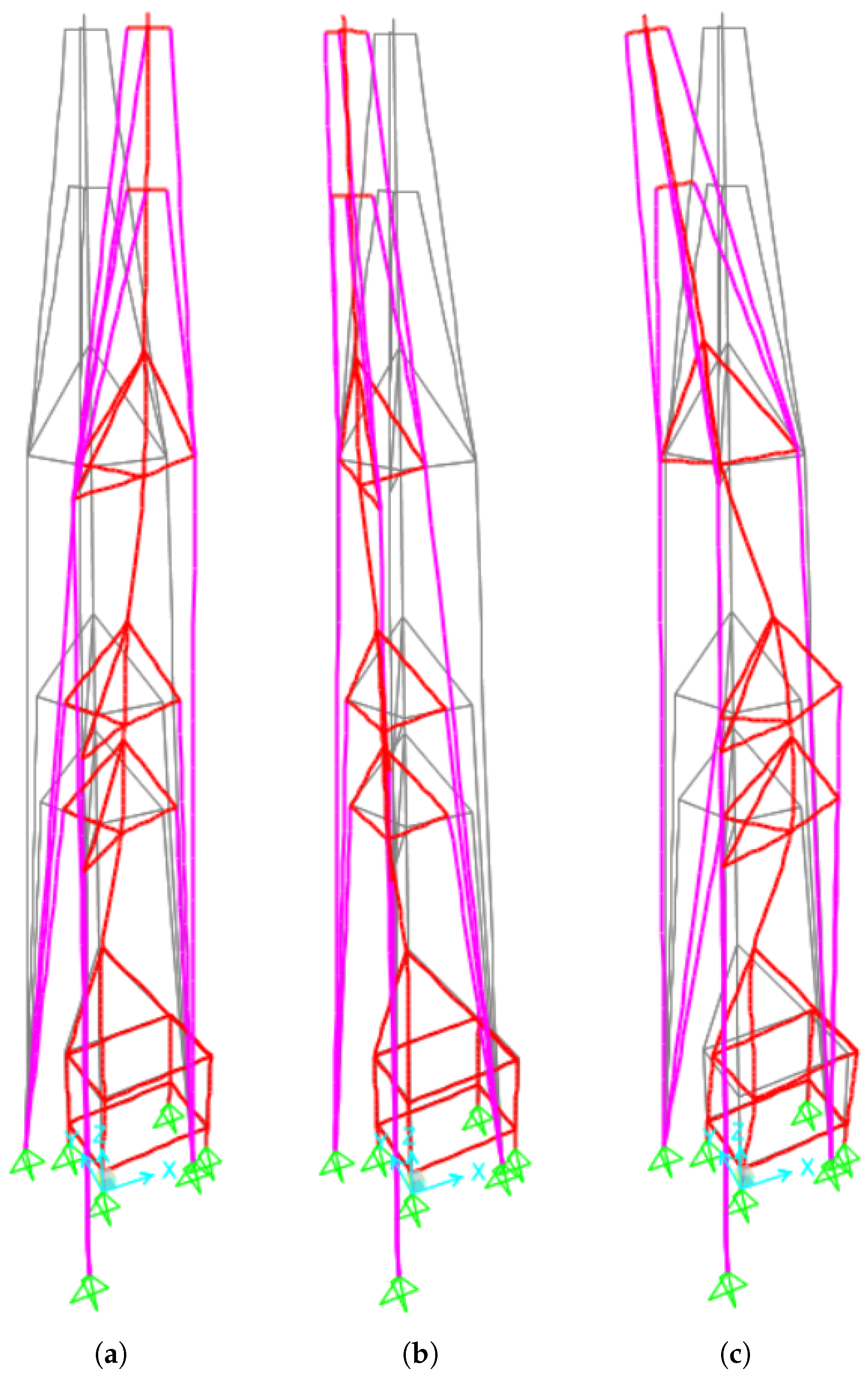
Figure 5 plots the three modes with a higher mass participation ratio. These are the 10th, 11th, and 12th modes obtained from the dynamic analysis of the mast structure with the dead loads. On the contrary, the first modes arising from the dynamic analysis have lower mass participation factors and are characterized by local deformation of the structural elements. The 10th, 11th, and 12th modes are the first modes exhibiting the global deformation of the mast structure.

X and Y identify the in-plane orthogonal directions. The 10th and 11th modes have an approximate 26% mass participation factor in the Y and X directions, respectively. The natural period is very low and at approximately 0.4 s. The 13th mode is mainly torsional with nearly a 7 and 4% mass participation factor in the X and Y directions.

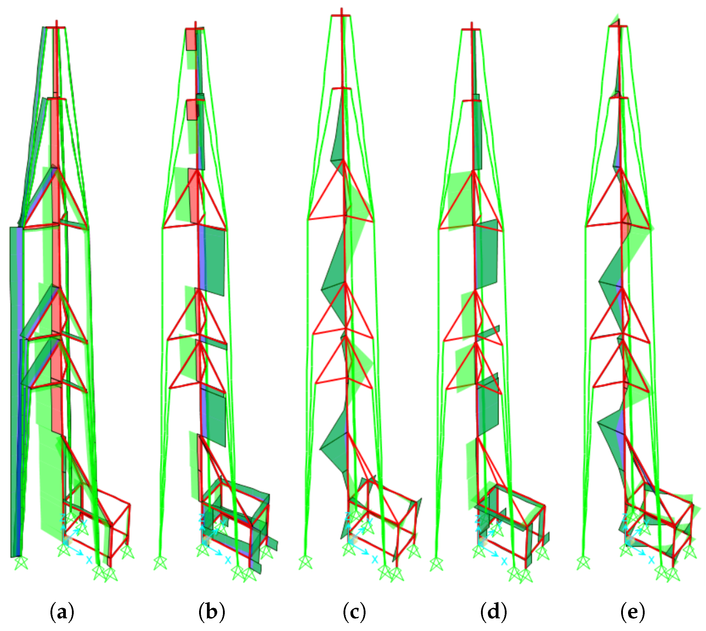
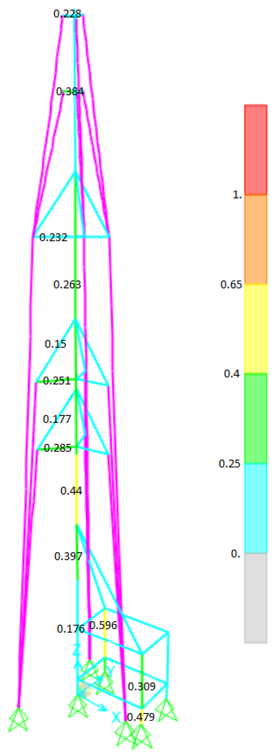
Figure 6 shows the positive (in dark green and purple) and negative (in red and light green) maximum and minimum envelopes of the axial, shear forces, and bending moments acting on the structural elements. Figure 7 plots the performance ratios of all structural elements except for the cables. The performance ratio is the ratio between the maximum stress in the structural element and the yielding stress. The performance ratios are defined by the colour map next to Figure 7. The plots highlight the presence of a structural element in the first half of the central pole with a high-performance ratio, depicted in yellow. The first section of the central pole has a low performance ratio, lower than 0.25. After the section with a performance ratio in the range 0.4–0.65, the following sections fall in the range 0.25–0.4 and are coloured in green. The top sections of the central pole are not significantly stressed, with a performance ratio of 0–0.25. The bracings have low stress, plotted in cyan, with performance ratios of 0–0.25.

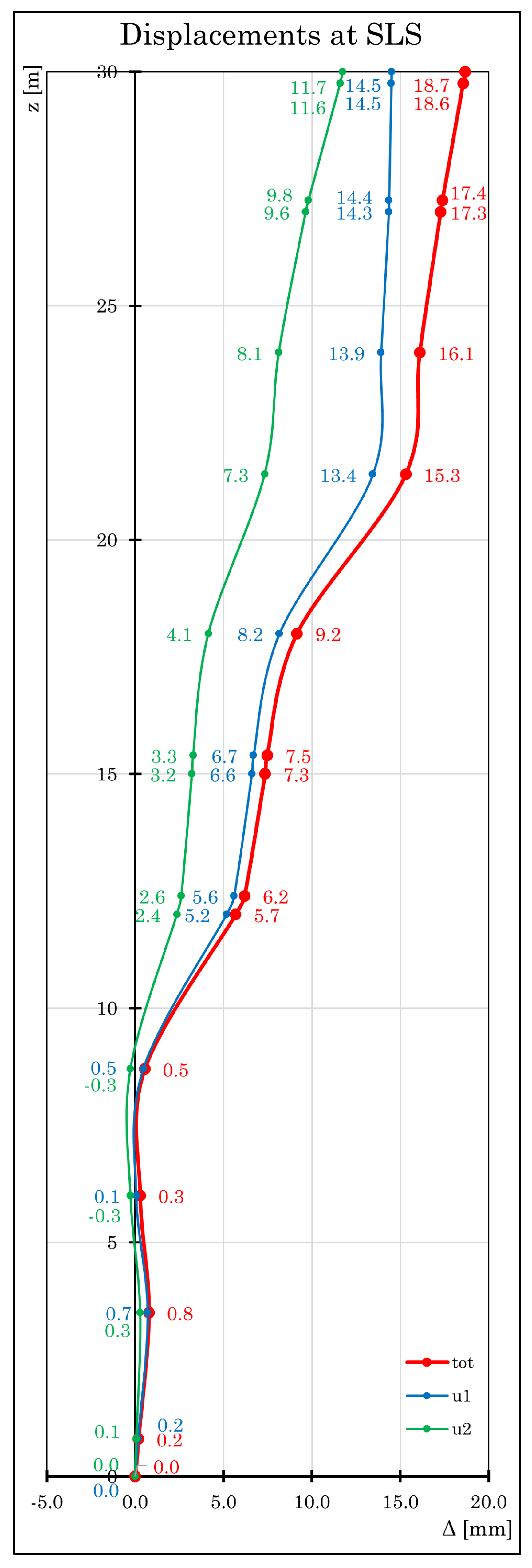
Figure 8 shows the maximum displacements in the X ($u_1$), Y ($u_2$) directions and their combination ($u_t$) at the service limit state. The maximum displacement is located at the top of the tower, in particular at joint 6 (z = 30.00 m), with a maximum displacement equal to $u_t$ = 18.7 mm.

5. Structural Optimization

In optimization problems, the main goal is to find the best conditions in terms of the optimal set of design parameters collected in the design vector $\mathit{x}$, which minimizes an objective function (OF) $f\left(\mathit{x}\right)$ [45,46,47]. These problems can be categorized into single-objective or multi-objective based on the number of OFs involved, and a further classification is based on the presence (or not) of constraints [48,49,50]. In the structural optimization field, it is common to deal with constrained optimization, whose general statement is [51]:

$$\begin{array}{cc}\hfill \hfill & \underset{\mathit{x}\in \mathsf{\Omega }}{min}\left\{f\left(\mathit{x}\right)\right\}\hfill \\ \hfill \mathrm{s}.\mathrm{t}.\hfill & g_q\left(\mathit{x}\right)\le 0\forall q=1,\dots ,n_q\hfill \\ \hfill \hfill & h_r\left(\mathit{x}\right)=0\forall r=1,\dots ,n_r\hfill \end{array}$$

(4)

where $\mathit{x}={\{x_1,\dots ,x_j,\dots ,x_n\}}^T$ is the design vector to be optimized, whose terms are limited into a hyper-rectangular multidimensional box-type search space domain of interest denoted as $\mathsf{\Omega }$, given by the Cartesian product of the range of interest of each j-th of each design variable bounded in $[x_j^l,x_j^u]$, $\mathsf{\Omega }=[x_1^l,x_1^u]\times \dots \times [x_j^l,x_j^u]\times \dots \times [x_n^l,x_n^u]$. The term $g_q\left(\mathit{x}\right)$ in (4) denotes inequality constraints whereas $h_r\left(\mathit{x}\right)$ are equality ones, which further reduce the feasible search space inside $\mathsf{\Omega }$. In structural optimization, it is typical to deal with inequality constraints, and a common goal is to minimize the global cost of the structure. Since this involves many terms, the main attempt is minimizing the self-weight of the structure, indirectly connected to material cost, i.e., material usage and natural resources consumption [51]. Several strategies have been developed over the years to handle constraints [52,53,54]. In the present work, the penalty function-based approach was implemented due to its simplicity, allowing converting the problem with OF $f\left(\mathit{x}\right)$ into a new unconstrained version $\varphi \left(\mathit{x}\right)$:

$$\underset{\mathit{x}\in \mathsf{\Omega }}{min}\left\{\varphi \left(\mathit{x}\right)\right)\}=\underset{\mathit{x}\in \mathsf{\Omega }}{min}\{f\left(\mathit{x}\right)+H\left(\mathit{x}\right)\}$$

(5)

where $H\left(\mathit{x}\right)$ is the penalty function. Adopting a static-penalty strategy, $H\left(\mathit{x}\right)$, assume this form [55,56]

$$H_s\left(\mathit{x}\right)=w_1{H}_{NVC}\left(\mathit{x}\right)+w_2{H}_{SVC}\left(\mathit{x}\right)$$

(6)

where $H_{NVC}$ is the number of violated constraints and $H_{SVC}$ is the sum of all violations:

$$H_{SVC}\left(\mathit{x}\right)=\sum _{p=1}^{n_p}max\{0,g_p\left(\mathit{x}\right)\}$$

(7)

$w_1$ and $w_2$ are the violation control parameters, whose numerical values are assumed equal to $w_1=w_2=100$ following [55].

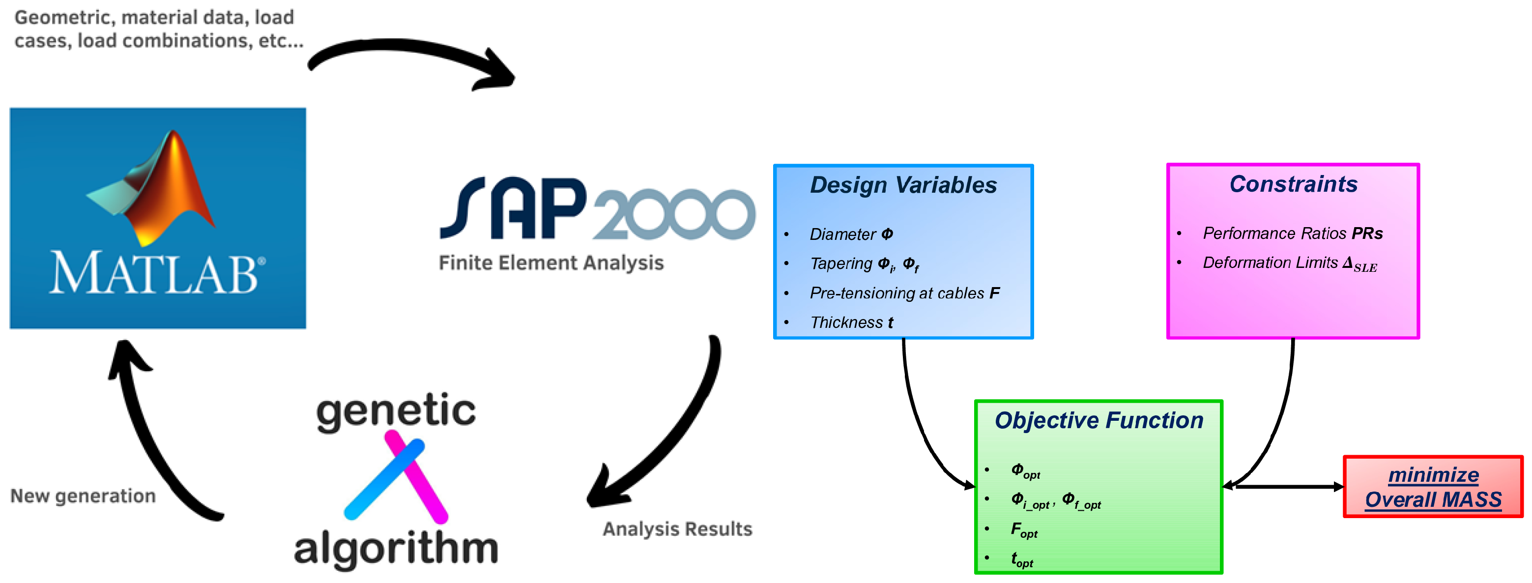
In the current study, the authors carried out a parametric study on the design variables of the guyed mast. This fact has led to eight different scenarios, summarized in

Table 5. Parametric study on the design variables involved and summary of the different scenarios.

Scenario	No. Parameters
A ($\mathsf{\Phi }$)	1
B (${\mathsf{\Phi }}_i,{\mathsf{\Phi }}_f$)	2
C (${\mathsf{\Phi }}_i,{\mathsf{\Phi }}_f,F$)	3
D (${\mathsf{\Phi }}_i,{\mathsf{\Phi }}_f,t$)	3
E (${\mathsf{\Phi }}_i,{\mathsf{\Phi }}_f,t,F$)	4
F (${\mathsf{\Phi }}_i,{\mathsf{\Phi }}_f,t_{ends},t_{inter},F$)	5
G ($t_1,t_2,t_3,t_4,t_5$)	5
H (${\mathsf{\Phi }}_i,{\mathsf{\Phi }}_f,t_1,t_2,t_3,t_4,t_5$)	8

. In addition, the starting initial values of the design parameter are listed in

Table 6. Total mass of the main pole.

Parameter	Measure	Value
${\mathsf{\Phi }}_0$	[mm]	168.3
$t_0$	[mm]	12.5
L	[mm]	6000
Mass	[kg]	288
no elements	[-]	5
Total Mass	[kg]	1440

, while the general optimization workflow is illustrated in Figure 9. To compare the results, the focus is related only to the performance ratios PR of the central pole of the guyed radio mast, being the pole the most stressed element. It consists of five segments 6.00 m long with the same cross-section. Thus, starting from the ground level:

• Pole${}_1$ (0.00 to 6.00 m);
• Pole${}_2$ (6.00 to 12.00 m);
• Pole${}_3$ (12.00 to 18.00 m);
• Pole${}_4$ (18.00 to 24.00 m);
• Pole${}_5$ (24.00 to 30.00 m).

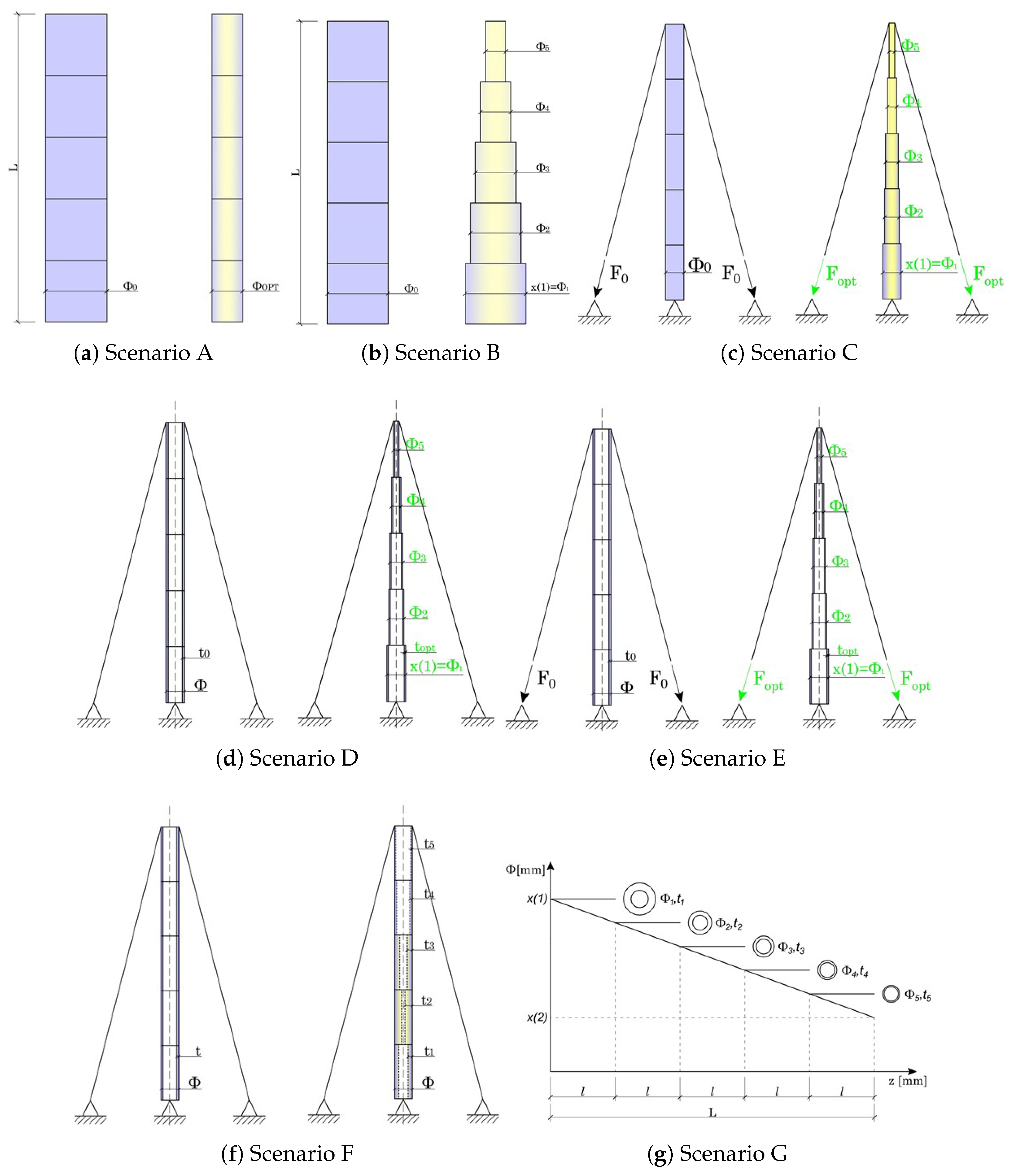
Starting with a constant diameter of the cross-section for the pole, at the end of the optimization, it is advisable to find a tapered solution following a linear relationship with the height, as represented in Figure 10f. Accordingly, it is possible to shape the pole cross-section with two design variables described by the bottom ${\mathsf{\Phi }}_i$ and top ${\mathsf{\Phi }}_f$ diameters. In the following, the different scenarios obtained from the parametric study based on the design variables involved in the optimization problem are described:

• Scenario A: this scenario involves the diameter $\mathsf{\Phi }$, as a sole variable, in the attempt to reduce the material consumption with a constant pole cross-section diameter with the height, as illustrated in Figure 10a.
• Scenario B: this scenario attempts to refine the previous case by adopting a tapered solution for the pole, by using the bottom ${\mathsf{\Phi }}_i$ and the top ${\mathsf{\Phi }}_f$ diameters, as represented in Figure 10b.
• Scenario C: further improvements are considered concerning scenario B by adding the cable pre-stressing force F as a variable of the optimization, as represented in Figure 10c.
• Scenario D: further improvements are considered to scenario B by using a unique value for the pole thickness t of the tapered elements of the pole, as represented in Figure 10c.
• Scenario E: further improvements are considered with respect to scenario B by optimizing both cable pre-stressing force F with a unique value of thickness t for the tapered elements of the pole, as represented in Figure 10e.
• Scenario F: from the structural analysis of scenario E, it is possible to point out how the linear law for the tapering forces to use a larger section where it is not necessary. Elements 2 and 3 are the most stressed ones. Therefore it is possible to further refine scenario E by considering a thickness value for the intermediate pole elements $t_{inter}$ and a different thickness for the other extremal pole elements $t_{e}nds$.
• Scenario G: in this scenario, the five different thickness values only have been governed for every pole element $\{t_1,t_2,t_3,t_4,t_5\}$ for a constant diameter solution with height, as depicted in Figure 10f.
• Scenario H: in this last scenario, a complete approach involves both the tapered solution by governing the initial bottom ${\mathsf{\Phi }}_i$ and the final top ${\mathsf{\Phi }}_f$ diameters, the five values of thickness for every pole element $\{t_1,t_2,t_3,t_4,t_5\}$, and even the cable pre-stressing force.

Constraints Involved in the Structural Optimization Problem

The optimization problem statement is reported in (4) and the constraints were treated with the penalty-based approach illustrated in (5), by converting the constrained problem into an equivalent unconstrained one. The resolution of the optimization task considers the structural design assessment required by national and international codes to ensure the safety of constructions. In particular, the structural verifications derive from Eurocode 3 (EN 1993-1-1: 2005) and are referred to the ultimate limit state (ULS). The design verifications include tensile, compression, and buckling verification, and a combined assessment, such as the interaction capacity according to Annex B of the Eurocode 3:

$$\begin{array}{cc}\hfill \frac{D}{C}\hfill & =\frac{N_{Ed}}{\frac{{\chi }_{y}A{f}_{yk}}{{\gamma }_{M1}}}+k_{yy}\frac{M_{y,Ed}}{\frac{{\chi }_{LT}{W}_{pl,y}{f}_{yk}}{{\gamma }_{M1}}}+k_{yz}\frac{M_{z,Ed}}{\frac{W_{pl,z}{f}_{yk}}{{\gamma }_{M1}}}\le 1\hfill \end{array}$$

(8)

$$\begin{array}{cc}\hfill \frac{D}{C}\hfill & =\frac{N_{Ed}}{\frac{{\chi }_{z}A{f}_{yk}}{{\gamma }_{M1}}}+k_{zy}\frac{M_{y,Ed}}{\frac{{\chi }_{LT}{W}_{pl,y}{f}_{yk}}{{\gamma }_{M1}}}+k_{zz}\frac{M_{z,Ed}}{\frac{W_{pl,z}{f}_{yk}}{{\gamma }_{M1}}}\le 1\hfill \end{array}$$

(9)

where D stands for the demand and C stands for the capacity of the structure. Specifically, $N_{Ed}$ is the acting axial force, whereas $M_{y,Ed}$ and $M_{z,Ed}$ represent the acting bending moments in the two principal directions of a planar local reference system centered on the cross section center of gravity. A is the cross section area of the pole, $W_{pl,y}$ and $W_{pl,z}$ are the plastic section modulus in the two principal directions, $f_{yk}$ is the yielding strength of the steel, whereas ${\gamma }_{M1}$ is the partial safety factor for instability conditions, equal to 1.05 from the Italian National Annex. ${\chi }_{LT}$ is the reduction factor for lateral–torsional buckling, whereas $kyy$, $kyz$, $kzy$, and $kzz$ are interaction factors whose values are derived according to two alternative approaches based on Annex A (method 1)and Annex B (method 2). The global structural deformation referred to the service limit state (SLS) has also been considered by verifying the top displacement of the mast. Specific recommendations for guyed mast structures are missing in national and international codes. Therefore, the authors adopted the suggestions defined in the Italian Technical Code NTC2018 (D.M.17/01/2018) reported in Chapter 4.2.4.2.2 Table 4.2.XIII related to limitations of lateral displacements of steel multi-storey frame structures. These limitations express a threshold condition in terms of the total height of the structure H:

$${\delta }_{\mathrm{SLS},\mathrm{top}}\le {\delta }_{\mathrm{SLS},\mathrm{top},\lim }=\frac{H}{500}=\frac{30000\mathrm{mm}}{500}=60\mathrm{mm}$$

(10)

Since this condition is specific for steel multi-storey frame structures, the authors will assume this value as a reasonable choice to ensure service life assessment and preservation of working conditions of the telecommunication guyed mast tower. In the next section, a discussion on the results is carried out.

6. Results and Discussion

The paper compares the outcomes of the size and shape optimization in eight different scenarios, distinguished by different design variables. Scenario A is associated with the worst improvement of the structural performance since a single diameter is used for the central pole. Additionally, industrial steel profiles do not cover all possible ranges of the diameter. Improvements in the structural performance and weight reduction are achieved in the following scenarios when the search space becomes larger by increasing the number of design variables.

Scenario B introduces the tapering of the central pole with a linear variation from the bottom to the top. In this case, the optimal solution is affected by intermediate sections, which are more stressed. Consequently, the end cross-sections are over-estimated. In response to that, Scenario F introduces the linear tapering of the tube thickness $t_{ends}$, $t_{inter}$ to enhance the performance of the optimal solution. Parallelly, in Scenario G, five different thicknesses are adopted ($t_1$, $t_2$, $t_3$, $t_4$, $t_5$), and the results are analogue to case F. Therefore, the thickness of the steel members is a suitable optimization parameter. At the same time, the diameter alone is not capable of returning attractive solutions because a linear interpolation trend is used. In addition, lower and upper limits were imposed for d and t. In particular, for this kind of structure, a minimum diameter $d_{min}\ge$ 100 mm and a minimum thickness $t_{min}\ge 3$ mm was imposed.

The cross-section area depends on the square of the thickness. Therefore, small changes in t significantly affect the resulting area. Conversely, if the diameter is the sole search space, despite being tapered linearly with height, even significant modifications may not produce notable improvements. Still, the increment of design variables involved in the structural optimization typically increases the computational efforts. However, the scenario with the highest number of variables was characterized by an average time iteration close to 18s, using a computer with average performance. The computational effort cost of the optimization procedure strongly depends on the machine performance, no convergence issues occur.

Table 7. Averaged performance ratios obtained in each optimization scenario.

No Parameters	PR Initial	PR Optimized	PR Design
	[%]	[%]	[%]
1	28.0	45.7	40.5
2		39.5	43.1
3		50.5	50.6
4		54.4	58
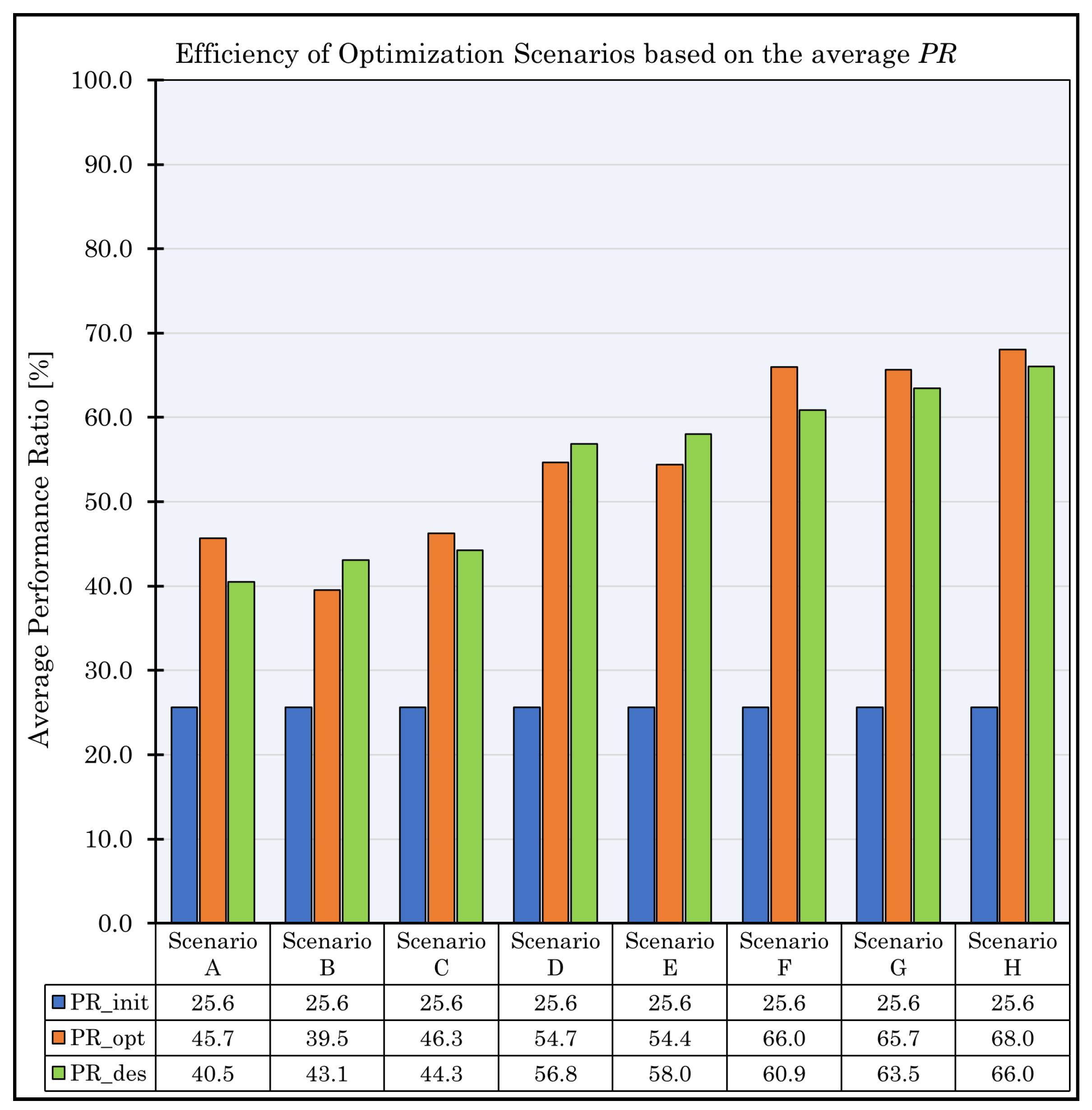
5		65.8	60.2
8		68	66

lists the average values of performance ratio obtained from the eight optimization scenarios. All scenarios were collected in terms of number of parameters involved during the analysis. Table 7 proves that the increment in the number of design variables is associated with higher performance ratios. The target of the optimization achieves the best weight reduction, fully exploiting the structural material, without exceeding the ultimate and service limit states. Table 7 lists three sets of performance ratios: the initial one before optimization, the optimized, and the one obtained using commercial steel profiles, called the design performance ratio. The averaged performance ratio is equal to 28% before optimization. It significantly increases from scenario A, nearly 45%, to scenario G with 68%.

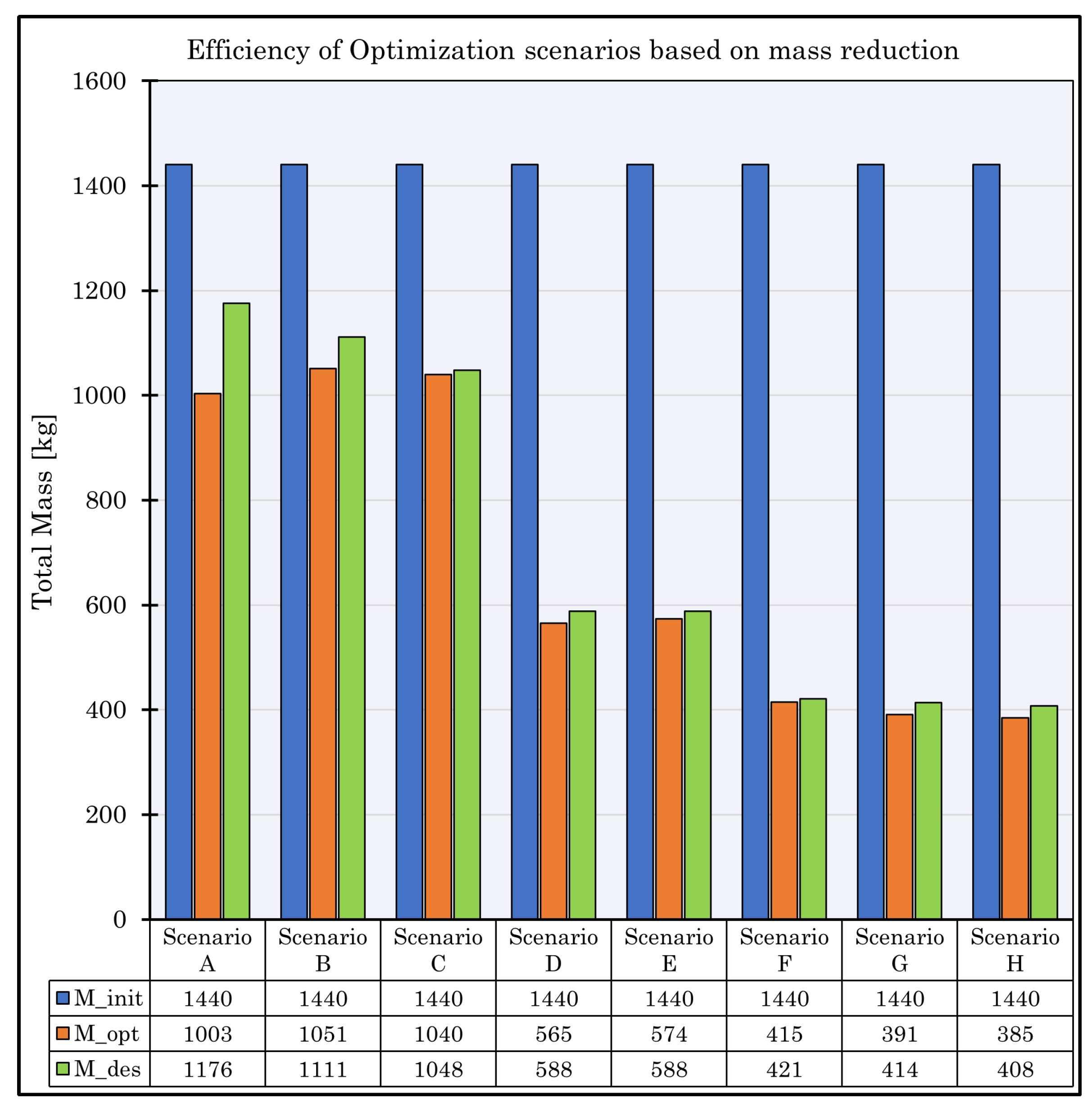
Essentially related to PR, mass reduction gives an idea about how much lighter (or heavier) the structure becomes due to the optimization process. It directly provides an estimate of cost savings.

Therefore, the results in

Table 8. Mass values before/after optimization and after proper approximation (design) using commercial steel profiles.

No Parameters	Initial Mass [kg]	Optimized Mass [kg]	Design Mass [kg]
1	1440	1003	1176
2		1051	1111
3		803	818
4		574	588
5		403	453
8		385	408

are consistent with the ones in terms of performance ratios, shown in Table 7.

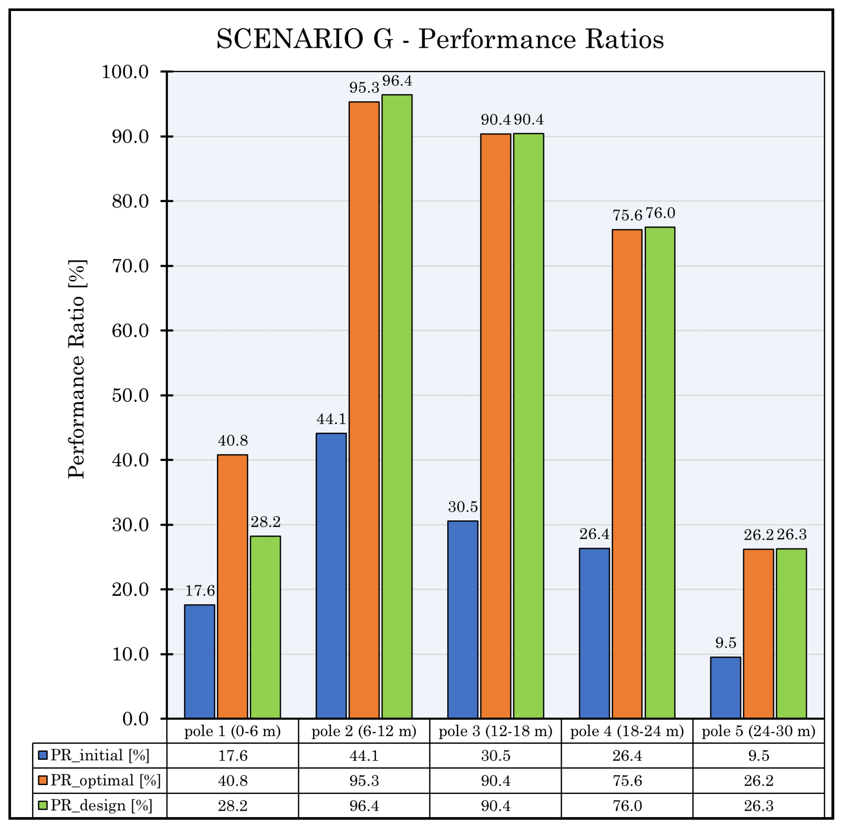
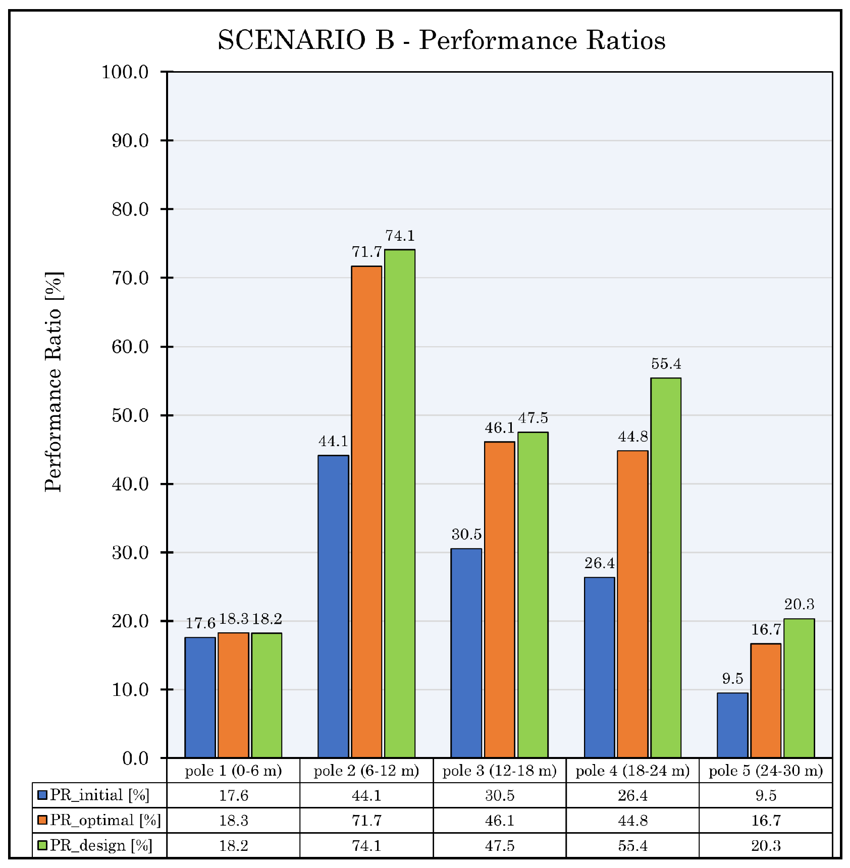
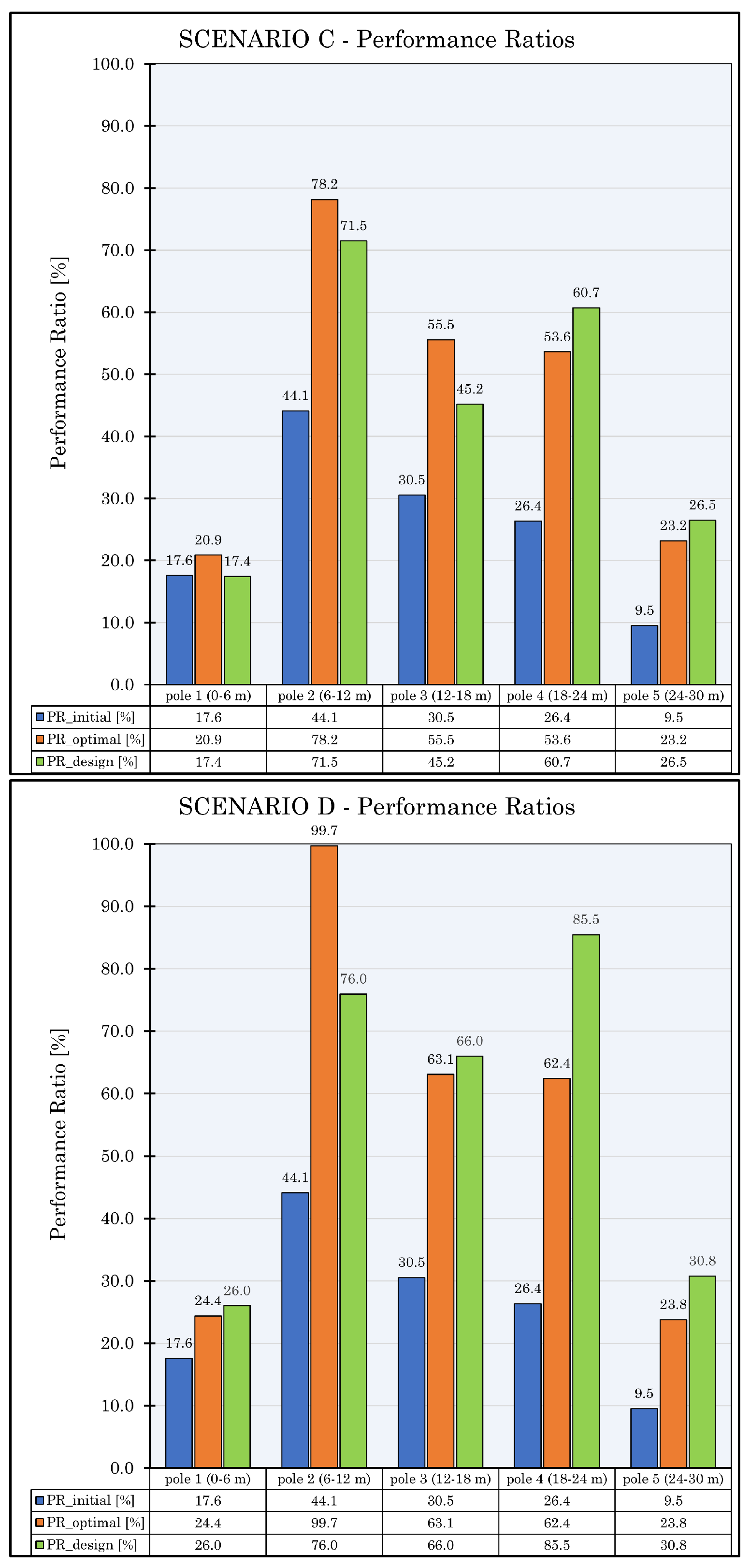
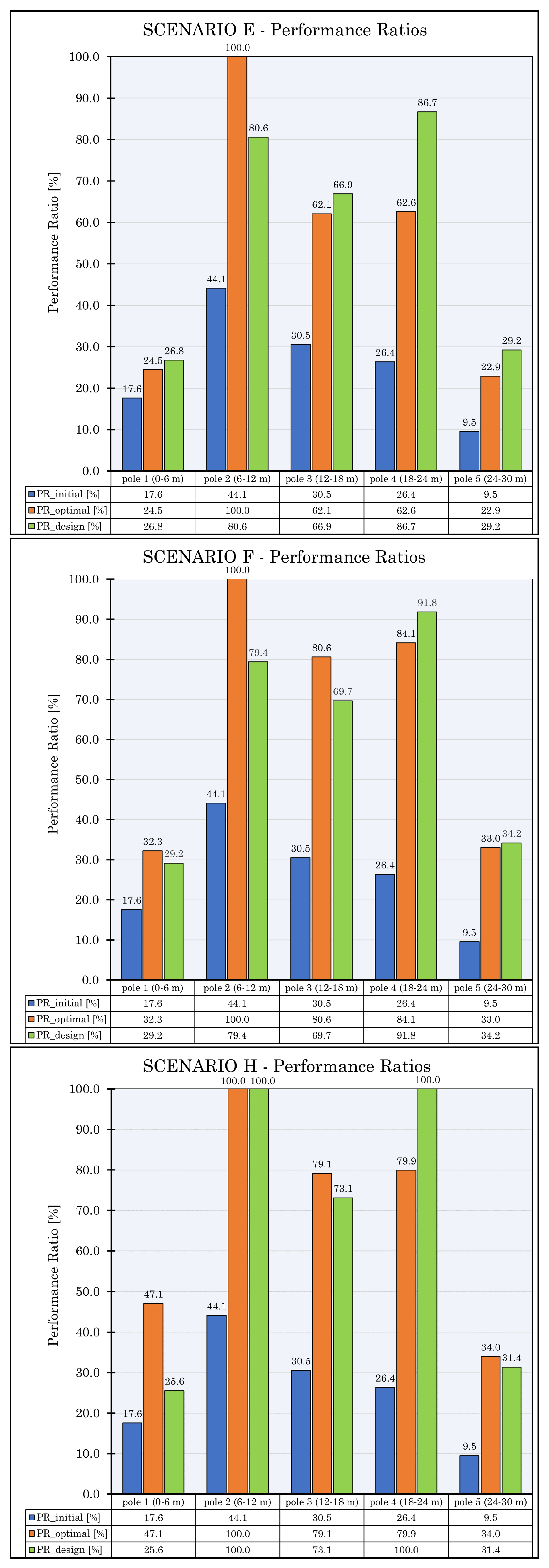
Figure 11 shows the optimization results for the Scenario G, in term of the performance ratio obtained by averaging the performance ratios for each structural element. The results for all scenarios are reported in Appendix A. Scenario G, depicted below, exhibits higher values of the performance ratios. This fact becomes become more evident for poles 2, 3, and 4. In these cases, the performance ratios, associated with the design solutions, achieved values equal or greater than the optimized one due to the approximation of the design section adopted. In the post-processing phase, in fact, the optimized section chosen by the list of the FE software was manually edited since the structural constraint violation or the maximum performance ratio was not reached during to the optimization process. Moreover, in

Table 9. Scenario G results: optimized solutions for the different independent executions (Ntrial) and proposed industrial one, according to the product list.

SCENARIO G—Optimized Solution
Element	d [mm]	t [mm]	L [mm]	Mass [Kg]
Pole 1 (0–6 m)	168.3	3	6000	73
Pole 2 (6–12 m)	168.3	4	6000	97
Pole 3 (12–18 m)	168.3	3	6000	73
Pole 4 (18–24 m)	168.3	3	6000	73
Pole 5 (24–30 m)	168.3	3	6000	73
Total Mass [kg]			$\mathsf{\Sigma }$	391
Mass variation [kg]	−1050	Mass variation [%]		−72.88
SCENARIO G—Design proposed according to the product list
Element	d [mm]	t [mm]	L [mm]	Mass [Kg]
Pole 1 (0–6 m)	168.3	4	6000	97
Pole 2 (6–12 m)	168.3	4	6000	97
Pole 3 (12–18 m)	168.3	3	6000	73
Pole 4 (18–24 m)	168.3	3	6000	73
Pole 5 (24–30 m)	168.3	3	6000	73
Total Mass [kg]			$\mathsf{\Sigma }$	414
Mass variation [kg]	−1026	Mass variation [%]		−71.22
Ntrial = 3
$t_1$	$t_2$	$t_3$	$t_4$	$t_5$	OF
[mm]	[mm]	[mm]	[mm]	[mm]	[kN]
3	4	4	3	3	34.985
3	4	3	3	3	34.751
3	4	3	4	3	34.985

, the optimized design section for different independent iterations and the proposed industrial solutions according to product list, provided by the software, are listed. As expected, the mass reduction achieved during the optimization process results higher than the design solution due to the approximation issue. For the proposed scenario, the iteration ($N_{trial}$) that guarantees the best objective function is the second. In Appendix A, the graphical (through histogram charts) and numerical representation (through tables) of the optimization result for each scenario are provided. In order to provide an overview of the objective function trend, the performance ratios and mass reduction for each scenario were collected into Figure 12 and Figure 13. The mentioned values were obtained for each scenario, making an average of the results, before and after optimization, independently, for each steel profile composing the central pole.

Figure 12 highlights an almost monotone increment of the performance ratios to the number of design variables. Interestingly, for a number of variables n ≥ 5, no significant improvements are achieved. Figure 13 emphasizes an important reduction of structural mass as the design variables increase. Once again, n = 5 represents trade-off. If the number of variables exceed 5, no significant improvements are observed.

Figure 12 and Figure 13 show a comparison between each scenario in terms of the average performance ratio and mass reduction, respectively. Figure 12 highlights the difference with the initial state, which has an average performance ratio $P{R}_0$ = 25.6%. An evident improvement is achieved for scenarios that include the thickness t as the design variable.

In particular, from Scenarios D, E, F, G, H, the average performance ratios exceed 50%, resulting in a more than 40% difference compared to the initial state. Figure 12 shows that the commercial profiles are sufficient to accommodate the optimized solution. An exception is noticeable in Scenario A because the optimization is performed using just one diameter $\mathsf{\Phi }$, which is optimal for a few parts of the structure, while others are “over-fitted”, resulting in a decrease of the performance ratios −28.4% and an increase of structural mass (+173 kg), as shown in Figure 13.

Similarly, a monotonic increment of the structural mass at the end of the optimization process is evident from Figure 13. In this case, the tonnage decreases with the increasing of the parameter’s number. There is an overall mass reduction of about −67.5% (−972 kg) from scenario D to H. In scenarios A, B, and C, the thickness t of structural members is not considered. Therefore, the mass loss is not satisfactory, at about −28.4% (−409 kg). The choice of the best scenario should depend on one of the five situations described above (from D to H) related to the better PRs gain and mass loss.

7. Conclusions

In this paper, a guyed radio mast’s size and shape optimization process was carried out to identify the equilibrium solution that guarantees the lighter optimized model, verifying strength, instability, and deformation requirements. The paper considers a detailed evaluation of the variable loads according to the Eurocodes recommendations. Furthermore, the OAPI was used to perform a structural analysis with the finite element software SAP2000 by considering the non-linearity of the cables. The optimization was carried out using a genetic optimization algorithm. Eight scenarios (labeled from A to H) were investigated, considering different arrangements of the geometric characteristics of the central pole and cables. The input parameters were increased from Scenario A to H to achieve the best fitness value of the self-weight. From Scenario A to H, the mass reduction index generally increased with the computational effort except in scenarios B and E, in which the input parameter did not represent the best vector design for the structural optimization. At this stage, the best design solution was evaluated from the database of cross-sections inside the finite element software. Though Scenario A provides the worst structural solution in terms of objective function, it represents the most convenient optimization strategy due to its low computational effort; on the contrary, Scenario H exhibits the best fitness value with the lowest self-weight, but it represents the most time-consuming solution. The best solution is achieved when the thickness values of each member, which, composed of the central pole, are included in the optimization process. An improvement of the structural behaviour against instability is observed with increasing thickness. This verification is critical for this structure, mainly subjected to normal stresses resulting from self-weight and pre-stressing cable force. The entire optimization process seems to not be sensible to the pole diameter, chosen as the input parameter of the design vector. Although the final results of the FEM analyses are based on the Italian standards, other codes (e.g., Eurocodes, American code, etc.) can be selected from the SAP2000 settings. However, since no detailed analysis was carried out and many standards are based on the semi-probabilistic approach, the final results should be similar, even with different code formulations. Nevertheless, the partial safety factors involved in load combinations remain quite the same from the numerical point of view, regardless of the followed code.

In future developments, the authors will attempt to replace circular hollow sections with built-up steel solutions to achieve the best structural performance and assemblage procedures. Especially for higher structures, guyed radio masts generally consist of a truss skeleton. Another possible development could be a structural optimization for a cable-stayed radio antenna adopting other optimization strategies, such as particle swarm optimization, PSO, and the evolution differential algorithm (EDA), which could be less time-consuming. Finally, it could perform a typological optimization by managing the position of the cable connection, trying to find the best attachment points.

References

1. Law, S.; Bu, J.; Zhu, X.; Chan, S.L. Wind characteristics of Typhoon Dujuan as measured at a 50 m guyed mast. Wind Struct. 2006, 9, 387–396. [Google Scholar] [CrossRef]
2. Sparling, B.; Wegner, L. Estimating peak wind load effects in guyed masts. Wind Struct. 2007, 10, 347–366. [Google Scholar] [CrossRef]
3. Hensley, G.M.; Plaut, R.H. Three-dimensional analysis of the seismic response of guyed masts. Eng. Struct. 2007, 29, 2254–2261. [Google Scholar] [CrossRef]
4. Amiri, G.G. Seismic sensitivity indicators for tall guyed telecommunication towers. Comput. Struct. 2002, 80, 349–364. [Google Scholar] [CrossRef]
5. Liu, C.; Fang, D.; Zhao, L. Reflection on earthquake damage of buildings in 2015 Nepal earthquake and seismic measures for post-earthquake reconstruction. Structures 2021, 30, 647–658. [Google Scholar] [CrossRef]
6. Sun, X.; Tao, X.; Duan, S.; Liu, C. Kappa (k) derived from accelerograms recorded in the 2008 Wenchuan mainshock, Sichuan, China. J. Asian Earth Sci. 2013, 73, 306–316. [Google Scholar] [CrossRef]
7. Buchholdt, H.; Moossavinejad, S.; Iannuzzi, A. Non-Linear Dynamic Analysis of Guyed Masts Subjected to Wind and Guy R Uptures. Proc. Inst. Civ. Eng. 1986, 81, 353–395. [Google Scholar] [CrossRef]
8. Ballaben, J.S.; Guzmán, A.M.; Rosales, M.B. Nonlinear dynamics of guyed masts under wind load: Sensitivity to structural parameters and load models. J. Wind Eng. Ind. Aerodyn. 2017, 169, 128–138. [Google Scholar] [CrossRef]
9. Gerstoft, P.; Davenport, A. A simplified method for dynamic analysis of a guyed mast. J. Wind Eng. Ind. Aerodyn. 1986, 23, 487–499. [Google Scholar] [CrossRef]
10. de Souza, R.R.; Miguel, L.F.F.; Lopez, R.H.; Miguel, L.F.F.; Torii, A.J. A procedure for the size, shape and topology optimization of transmission line tower structures. Eng. Struct. 2016, 111, 162–184. [Google Scholar] [CrossRef]
11. Saudi, G. Structural assessment of a guyed mast through measurement of natural frequencies. Eng. Struct. 2014, 59, 104–112. [Google Scholar] [CrossRef]
12. Saxena, R.; Popplewell, N.; Trainor, P.; Shah, A. Vibrations of complex guyed towers. In Proceedings of the 12th Biennial Conference on Mechanical Vibration and Noise Control, Montreal, QC, Canada, 17–21 September 1989. [Google Scholar]
13. Novak, M.; Tanaka, H.; Davenport, A.G. Vibration of towers due to galloping of iced cables. J. Eng. Mech. Div. 1978, 104, 457–473. [Google Scholar] [CrossRef]
14. Wahba, Y.M.; Madugula, M.K.; Monforton, G.R. Shake Table for Dynamic Testing of Guyed Towers. In Building to Last; ASCE: Reston, VA, USA, 1997; pp. 353–357. [Google Scholar]
15. Madugula, M.K.; Wahba, Y.M.; Monforton, G.R. Dynamic response of guyed masts. Eng. Struct. 1998, 20, 1097–1101. [Google Scholar] [CrossRef]
16. Luzardo, A.C.; Parnás, V.E.; Rodríguez, P.M. Guy tension influence on the structural behavior of a guyed mast. J. Int. Assoc. Shell Spat. Struct. 2012, 53, 111–116. [Google Scholar]
17. Davenport, A.; Sparling, B. Dynamic gust response factors for guyed towers. J. Wind Eng. Ind. Aerodyn. 1992, 43, 2237–2248. [Google Scholar] [CrossRef]
18. Harikrishna, P.; Annadurai, A.; Gomathinayagam, S.; Lakshmanan, N. Full scale measurements of the structural response of a 50 m guyed mast under wind loading. Eng. Struct. 2003, 25, 859–867. [Google Scholar] [CrossRef]
19. Gioffrè, M.; Gusella, V.; Materazzi, A.; Venanzi, I. Removable guyed mast for mobile phone networks: Wind load modeling and structural response. J. Wind Eng. Ind. Aerodyn. 2004, 92, 463–475. [Google Scholar] [CrossRef]
20. Clobes, M.; Peil, U. Unsteady buffeting wind loads in the time domain and their effect on the life-cycle prediction of guyed masts. Struct. Infrastruct. Eng. 2011, 7, 187–196. [Google Scholar] [CrossRef]
21. Pezo, M.L.; Bakić, V.V. Numerical determination of drag coefficient for guyed mast exposed to wind action. Eng. Struct. 2014, 62, 98–104. [Google Scholar] [CrossRef]
22. Sparling, B.F. The Dynamic Behavior of Guys and Guyed Masts in Turbulent Winds. Ph.D. Thesis, Western University, London, ON, Canada, 1995. [Google Scholar]
23. Wahba, Y.; Madugula, M.; Monforton, G. Evaluation of non-linear analysis of guyed antenna towers. Comput. Struct. 1998, 68, 207–212. [Google Scholar] [CrossRef]
24. Madugula, M.K. Dynamic Response of Lattice Towers and Guyed Masts; ASCE Publications: Reston, VA, USA, 2001. [Google Scholar]
25. Orlando, D.; Gonçalves, P.B.; Rega, G.; Lenci, S. Nonlinear dynamics and instability as important design concerns for a guyed mast. In IUTAM Symposium on Nonlinear Dynamics for Advanced Technologies and Engineering Design; Springer: Berlin/Heidelberg, Germany, 2013; pp. 223–234. [Google Scholar]
26. Ballaben, J.S.; Rosales, M.B. Nonlinear dynamic analysis of a 3D guyed mast. Nonlinear Dyn. 2018, 93, 1395–1405. [Google Scholar] [CrossRef]
27. Belevičius, R.; Jatulis, D.; Šešok, D. Optimization of tall guyed masts using genetic algorithms. Eng. Struct. 2013, 56, 239–245. [Google Scholar] [CrossRef]
28. Gawronski, W.; Bienkiewicz, B.; Hill, R. Wind-induced dynamics of a deep space network antenna. J. Sound Vib. 1994, 178, 67–77. [Google Scholar] [CrossRef]
29. Fujino, Y.; Warnitchai, P.; Pacheco, B. Active Stiffness Control of Cable Vibration. J. Appl. Mech. 1993, 60, 948–953. [Google Scholar] [CrossRef]
30. Lacarbonara, W.; Ballerini, S. Vibration mitigation of guyed masts via tuned pendulum dampers. Struct. Eng. Mech. Int. J. 2009, 32, 517–529. [Google Scholar] [CrossRef]
31. Błachowski, B. Model based predictive control of guyed mast vibration. J. Theor. Appl. Mech. 2007, 45, 405–423. [Google Scholar]
32. Bell, L.C.; Brown, D.M. Guyed tower optimization. Comput. Struct. 1976, 6, 447–450. [Google Scholar] [CrossRef]
33. Thornton, C.H.; Joseph, L.; Scarangello, T. Optimization of tall structures for wind loading. J. Wind Eng. Ind. Aerodyn. 1990, 36, 235–244. [Google Scholar] [CrossRef]
34. Uys, P.; Farkas, J.; Jarmai, K.; Van Tonder, F. Optimisation of a steel tower for a wind turbine structure. Eng. Struct. 2007, 29, 1337–1342. [Google Scholar] [CrossRef]
35. Venanzi, I.; Materazzi, A. Multi-objective optimization of wind-excited structures. Eng. Struct. 2007, 29, 983–990. [Google Scholar] [CrossRef]
36. Zhang, Z.Q.; Li, H.N. Two-level optimization method of transmission tower structure based on ant colony algorithm. In Advanced Materials Research; Trans Tech Publications Ltd.: Freienbach, Switzerland, 2011; Volume 243, pp. 5849–5853. [Google Scholar]
37. Cucuzza, R.; Costi, C.; Rosso, M.M.; Domaneschi, M.; Marano, G.C.; Masera, D. Optimal strengthening by steel truss arches in prestressed girder bridges. In Proceedings of the Institution of Civil Engineers—Bridge Engineering; Thomas Telford Ltd.: London, UK, 2021; pp. 1–21. [Google Scholar] [CrossRef]
38. Luh, G.C.; Lin, C.Y. Optimal design of truss-structures using particle swarm optimization. Comput. Struct. 2011, 89, 2221–2232. [Google Scholar] [CrossRef]
39. Manuello Bertetto, A.; Marano, G. Numerical and dimensionless analytical solutions for circular arch optimization. Eng. Struct. 2022, 253, 113360. [Google Scholar] [CrossRef]
40. Kaveh, A.; Talatahari, S. Particle swarm optimizer, ant colony strategy and harmony search scheme hybridized for optimization of truss structures. Comput. Struct. 2009, 87, 267–283. [Google Scholar] [CrossRef]
41. Deng, Z.Q.; Zhang, Y.; Huang, H.L.; Li, B. Parametric optimization for a tapered deployable mast in an integrated design environment. In Advanced Materials Research; Trans Tech Publications Ltd.: Freienbach, Switzerland, 2012; Volume 346, pp. 426–432. [Google Scholar]
42. Guo, H.; Li, Z. Structural topology optimization of high-voltage transmission tower with discrete variables. Struct. Multidiscip. Optim. 2011, 43, 851–861. [Google Scholar] [CrossRef]
43. delle Ricerche, C.N. Istruzioni per la valutazione delle azioni e degli effetti del vento sulle costruzioni. CNR-DT 2009, 207, 2008. [Google Scholar]
44. Mordà, N.; Mancini, A. Norme Tecniche per le Costruzioni (NTC 2018) D. Min. Infrastrutture e Trasporti 17 Gennaio 2018; Ministero delle Infrastrutture e dei Trasporti: Roma, Italy, 2018. [Google Scholar]
45. Melchiorre, J.; Bertetto, A.M.; Marano, G.C. Application of a Machine Learning Algorithm for the Structural Optimization of Circular Arches with Different Cross-Sections. J. Appl. Math. Phys. 2021, 9, 1159–1170. [Google Scholar] [CrossRef]
46. Rosso, M.M.; Cucuzza, R.; Aloisio, A.; Marano, G.C. Enhanced Multi-Strategy Particle Swarm Optimization for Constrained Problems with an Evolutionary-Strategies-Based Unfeasible Local Search Operator. Appl. Sci. 2022, 12, 2285. [Google Scholar] [CrossRef]
47. Rosso, M.M.; Cucuzza, R.; Di Trapani, F.; Marano, G.C. Nonpenalty machine learning constraint handling using PSO-svm for structural optimization. Adv. Civ. Eng. 2021, 2021, 6617750. [Google Scholar] [CrossRef]
48. Rao, S.S. Engineering Optimization: Theory and Practice; John Wiley & Sons: Hoboken, NJ, USA, 2019. [Google Scholar]
49. Aloisio, A.; Pasca, D.P.; Battista, L.; Rosso, M.M.; Cucuzza, R.; Marano, G.; Alaggio, R. Indirect assessment of concrete resistance from FE model updating and Young’s modulus estimation of a multi-span PSC viaduct: Experimental tests and validation. Elsevier Struct. 2022, 37, 686–697. [Google Scholar] [CrossRef]
50. Sardone, L.; Rosso, M.M.; Cucuzza, R.; Greco, R.; Marano, G.C. Computational Design of Comparative models and geometrically constrained optimization of a multi-domain variable section beam based on Timoshenko model. In Proceedings of the EUROGEN2021, 14TH ECCOMAS Thematic Conference on Evolutionary and Deterministic Methods for Design, Optimization and Control, Athens, Greece, 28–30 June 2021. [Google Scholar] [CrossRef]
51. Christensen, P.W.; Klarbring, A. An Introduction to Structural Optimization; Springer Science & Business Media: Berlin/Heidelberg, Germany, 2008; Volume 153. [Google Scholar]
52. Coello Coello, C.A. Theoretical and numerical constraint-handling techniques used with evolutionary algorithms: A survey of the state of the art. Comput. Methods Appl. Mech. Eng. 2002, 191, 1245–1287. [Google Scholar] [CrossRef]
53. Koziel, S.; Michalewicz, Z. Evolutionary Algorithms, Homomorphous Mappings, and Constrained Parameter Optimization. Evol. Comput. 1999, 7, 19–44. [Google Scholar] [CrossRef] [PubMed]
54. Michalewicz, Z.; Fogel, D. How to Solve It: Modern Heuristics; Springer Science & Business Media: Berlin/Heidelberg, Germany, 2008. [Google Scholar]
55. Parsopoulos, K.; Vrahatis, M. Unified Particle Swarm Optimization for Solving Constrained Engineering Optimization Problems. In International Conference on Natural Computation; Springer: Berlin/Heidelberg, Germany, 2005; Volume 3612, pp. 582–591. [Google Scholar] [CrossRef] [Green Version]
56. Coello, C. Self-adaptive penalties for GA-based optimization. In Proceedings of the 1999 Congress on Evolutionary Computation-CEC99 (Cat. No. 99TH8406), Washington, DC, USA, 6–9 July 1999; IEEE: Hoboken, NJ, USA, 1999; Volume 1, pp. 573–580. [Google Scholar] [CrossRef]
Figure 1. (a) Render model realized using Tekla Structures. (b) Technical drawing of the structure investigated with dimensions in mm.
Applsci 12 04875 g001
Figure 2. Pictures and details of the considered structure.
Applsci 12 04875 g002
Figure 3. Mechanical stress–strain behaviour of steel S355 implemented in SAP2000.
Applsci 12 04875 g003
Figure 4. Elastic response spectrum corresponding to the service limit state (SLV), where S a is the spectral acceleration.
Applsci 12 04875 g004
Figure 5. (a) Mode 10th—Ts = 0.437 s—mass participation ratio X = 9.6%, Y = 26.2%; (b) Mode 11th—Ts = 0.434 s—mass participation ratio X = 26.4% Y = 9.2%; (c) Mode 12—Ts = 0.206 s—mass participation ratio X = 7.2% Y = 4.4%.
Applsci 12 04875 g005
Figure 6. (a) Axial force, (b) shear force ( V 2 ), (c) bending moment ( M 2 ), (d) shear force ( V 3 ), (e) bending moment ( M 3 ).
Applsci 12 04875 g006
Figure 7. Performance ratios of the pole before optimization. Cables are depicted with magenta colour because their performance ratios are not included in the current representation.
Applsci 12 04875 g007
Figure 8. Displacements vs. elevation at the service limit state in two in-plane orthogonal directions ( u 1 , u 2 ) and their combination (tot).
Applsci 12 04875 g008
Figure 9. Workflow of the optimization problem.
Applsci 12 04875 g009
Figure 10. Parametric study on the design variables involved and representation of the different scenarios described in Table 5.
Applsci 12 04875 g010
Figure 11. Scenario G.—PRs trend. In blue—the performance ratios of each pole before optimization are illustrated, otherwise orange for the optimized solution. In green—PRs at a design configuration according to the product list.
Applsci 12 04875 g011
Figure 12. In blue, orange, and green, the average PRs, respectively, at the initial condition, after optimization, and design solution.
Applsci 12 04875 g012
Figure 13. Increasing the number of design variables, the final mass becomes gradually smaller, until 385 kg (scenario H).
Applsci 12 04875 g013