Effect of the Distribution of Mass and Structural Member Discretization on the Seismic Response of Steel Buildings

Abstract

The response of steel moment frames is estimated by first considering that the mass matrix is the concentrated type (M_L) and then consistent type (M_C). The effect of considering more than one element per beam is also evaluated. Low-, mid- and high-rise frames, modeled as complex-2D-MDOF systems, are used in the numerical study. Results indicate that if M_L is used, depending upon the response parameter under consideration, the structural model, the seismic intensity and the structural location, the response can be significantly overestimated, precisely calculated, or significantly underestimated. Axial loads at columns, on an average basis, are significantly overestimated (up to 60%), while lateral drifts and flexural moments at beams are precisely calculated. Inter-story shears and flexural moments at columns, on average, are underestimated by up to 15% and 35%, respectively; however, underestimations of up to 60% can be seen for some individual strong motions. Similarly, if just one element per beam is used in the structural modeling, inter-story shears and axial loads on columns are overestimated, on average, by up to 21% and 95%, respectively, while the lateral drifts are precisely calculated. Flexural moments at columns and beams can be considerably underestimated (on average up to 14% and 35%, respectively), but underestimations larger than 50% can be seen for some individual cases. Hence, there is no error in terms of lateral drifts if M_L or one element per beam is used, but significant errors can be introduced in the design due to the overestimation and underestimation of the design forces. It is strongly suggested to use M_C and at least two elements per beam in the structural modeling.

1. Introduction

A considerable number of problems related to building analysis and design procedures have been studied for many years. For steel building structures subjected to strong earthquakes, modeling the stiffness (K), damping (C), and stiffness (K) matrices has not been the exception. The appropriate modeling of such matrices is a crucial step toward an accurate estimation of the seismic response. One of the most widely used structural systems in steel buildings is that based on moment-resisting frames (MRFs), where the prismatic framed-type members are represented by beam and beam-column members. It is essential to properly represent the aforementioned matrices, at both local and global levels, for this structural system.

The most common and simplest procedure to define the inertial properties of a building is to consider the mass as a concentrated type at the translational degrees of freedoms (DOFs) defined in the structure; it will result in a matrix (M_L) with non-zero numbers in the diagonal corresponding to such DOFs. It is possible, however, to derive a kinematically equivalent mass matrix called the consistent mass matrix (M_C) so inertia forces are also obtained for the rotational DOFs. It will give a matrix with values out of the diagonal, with the same band wide as the K matrix. Because of the better representation of the rotational inertia, it is expected that M_C will give more accurate results than M_L. It is also important to mention that in seismic analyses of steel MRFs, the M and K matrices are usually formulated by considering only one element to represent each structural member [1,2,3], which may introduce inaccuracy in the results.

Energy dissipation should also be properly estimated to correctly simulate the structural behavior. Since it can be generated from many sources, it is more important for steel structures. Due to its inherent complexity, this parameter is considered in building codes [4,5,6] by a linear viscous damper with equivalent damping of 5% of the critical (ζ = 5%), implying in general that the variation with the type of material or with the type of source is not explicitly identified. A significant number of investigations exist where energy dissipation produced by inelastic behavior of the material is represented by using a linear damper [7,8,9,10,11].

A more reasonable approach adopted in steel structures consists in modeling the dissipation of energy for small or moderated deformations (occurring within the elastic limit and termed as viscous energy) by a viscous damper, while that occurring at large deformations (termed as plastic energy) is considered by the constitutive law of the material. The traditional approach to consider the viscous energy has been through the Rayleigh Damping, which consists of expressing the matrix C as a combination of the M and K matrices. In this regard, two special cases of K need to be identified: the elastic (or initial) stiffness matrix (K_o) corresponding to small or moderate levels of deformations and the tangent stiffness matrix (K_t) corresponding to inelastic behavior.

In the analysis of MRFs under the action of large earthquakes, particular aspects as the second-order effects and the dissipation of energy at plastic hinges need to be captured in K_t. These issues are broadly discussed in the literature [2,12], particularly for prismatic members with straight axes, such as those used in the models of this study.

The effect of modeling the three abovementioned fundamental matrices has been broadly studied; however, as further discussed below, many problems require additional investigation. The primary objective of this research is to evaluate the responses of steel MRFs, considering different alternatives for the M matrix, as well as to evaluate the accuracy of considering one element to represent each beam.

2. Literature Review

A considerable number of research projects has been conducted to evaluate the effect of modeling of the M and C matrices on the response of structures [13,14,15,16]. Among the first works is that of Archer [17], who studied the effect of a consistent mass matrix for beams. Rea et al. [18] estimated the damping existing in some prototypes of special steel frame modes, which consisted of a platform supported by columns. Wilson and Penzien [19] developed two methods to numerically quantify the C matrix. Crisp [20] made a comparative analysis for different damping models to quantify their effect on the inelastic seismic response of reinforced concrete frames. Stavrinidis et al. [21], by using the Finite Element Method, proposed an improved version of the consistent mass matrix in terms of computational time for 1D and 2D members. Leger and Dussault [22] studied the influence of the mathematical representation of viscous damping on the dissipation of energy for structures modeled as MDOF systems. Hansson and Sandberg [23] presented a procedure to construct the M matrix, for the diagonal and the non-diagonal cases, by expressing it through a variable parameter. Gulkan and Alemdar [24] derived shape functions for segments of beams over a generalized foundation, which can be used to get exact equations to calculate the elements of the K and M matrices. Michaltsos and Konstantakopoulos [25], for the special case of a thin-walled tower, considered the effect of the rotational inertia of the structural members by adding additional concentrated masses. Kowalsky and Dwairi [26] analyzed the precision of using the equivalent viscous damper while used in the direct displacement-based design. Archer and Whalen [27] presented a procedure to diagonalize the M matrix considering translational and rotational DOFs. Val and Segal [28] calculated the responses of structures modeled as SDOF systems with viscous damping and compared them with those of hysteretic damping. Wu [29], by using linear elements with constant Jacobians, presented an approximation of the M matrix. Dwairi et al. [30] found considerable errors while applying the equivalent linearization of a nonlinear system for the case of the direct displacement-based design. Sarigul and Boyaci [31] studied the lateral displacements of beams with axial moving beams, having several concentrated masses. Zareian and Medina [32], in order to eliminate the problems associated to unrealistic large damping forces derived from the Rayleigh damping model, proposed an approach that consists in modeling the structural elements by a combination of one elastic element having damping proportional to the K matrix, and two springs at the ends with damping no proportional to K. Rodrigues et al. [33] proposed simplified expressions for viscous damping in R/C columns subjected to biaxial bending. Jehel et al. [34] compared the results of using the K_o stiffness matrix in the C matrix and compared the results with those of using the K_t. Analytical tools were provided to control damping ratios throughout inelastic analysis. Zuo et al. [35] identified the errors derived from the use of the M_L matrix and proposed a procedure to obtain M_L matrices for beam members containing both types of DOFs. Chai and Kowalsky [36] found an increment in the displacements of structures when exponential nonviscous damping was used in comparison with that of classical viscous damping. Deshpande et al. [37], for frequencies, estimated the responses of cantilever beams using the M_L matrix and compared such results with those of the M_C matrix. Puthanpurayil et al. [38] proposed a procedure to formulate the C matrix at an individual elemental level; to cases were considered to be applied in inelastic analysis. Ozel et al. [3] presented a procedure for steel frames, based on the Finite Element Method, to derive K and M matrices considering (a) the influence of deformations produced by shear forces, (b) rotational inertia of structural members and (c) the stiffness and dissipation of energy of semi-rigid connections. Pradhan and Modak [39] investigated damping matrix identification of structures via finite element model and normal frequency response functions. They successfully demonstrated their identification techniques using experimental studies. Carr et al. [40] described many inconveniences of the Rayleigh model when used in inelastic analyses and recommended a damping model which resembles the damping that is expected in nonlinear dynamic analysis. Zand and Akbari [41] analyzed the influence of several viscous damping models on the nonlinear response of concentrically braced and moment-resisting steel frames. Experimental and numerical studies to evaluate the natural frequencies of bones for supportive equipment used while walking and running conditions were conducted by Kshirsagar et al. [42].

The aforementioned investigations represent a big step toward the understanding of the effects of modeling the M and C matrices on the seismic response of buildings. However, many related aspects still need to be studied. There are indeed some studies where the structural responses are obtained by considering the M_L matrix and compared with those obtained by using the M_C matrix. However, it has not been done for the case steel buildings of different heights modeled by MDOF systems, for different local and global response parameters. The accuracy of calculating the response considering one, two, and three elements per member has not been investigated either. Some of these problems are studied in this research.

3. Objectives

In this research, the nonlinear responses of plane steel MRFs subjected to earthquakes, modeled as complex MDOF systems, are determined to study some problems related to the idealization of the M matrix. Low-, mid- and high-rise frames are analyzed for a range of earthquake excitations. The responses are expressed in terms of several parameters, namely, lateral drifts, inter-story shears, and axial loads and flexural moments at beams and columns. The particular issues addressed here are:

(a) Calculate the local and global responses of the used models by assuming that the mass matrix is concentrated type (M_L) and compare the results with those of considering such a matrix as consistent type (M_C).

(b) Study the effect on the response of considering one, two, or three elements per beam in the structure.

4. Methodology and Procedure

To meet the objectives abovementioned, the responses of three steel buildings are estimated by modeling them, as stated earlier, by complex 2D MDOF frames. Therefore, higher mode contributions are explicitly considered. Such models are subjected to the action of fifteen seismic records corresponding to the seismic hazard of the model location zone. The nonlinear analyses are performed with the Ruaumoko Software [43] where the Newmark Average Acceleration Method of Newmark with a time interval (Δt) of 0.005 s. is used. Large displacement effects are also considered in the dynamic analysis. The results of the M_L matrix are compared to those of M_C. The Rayleigh damping model is used, where the K_t matrix and 3% of viscous damping (ζ = 3%) are assumed in the construction of the damping matrix. This amount of damping is fixed in the first and second modes for the smaller model; such modes are 1 and 3, and 1 and 6 for the mid and high models, respectively.

Damping represents a very controversial issue within the seismic analysis of buildings. There is some available information regarding the evaluation of the damping ratio. From earthquake-vibration tests of buildings deformed below yield point [44] it was found that the damping ratio ranged from 2.9% to 7.0% for the first mode while the range of variation goes from 1.0% to 5.9% for the second mode. In the same reference, taking into account that other sources of energy dissipation are considered in the C_R matrix, conservative values of 2–3% and 5–7% are suggested for stress levels of half of yield, and yield point, respectively. In another research [45] it was found that for small amplitudes of vibration the damping ratio for the fundamental mode of vertical vibrations approximately varies from 2% to 5% for R/C buildings, and from 0.5% to 2% for the steel buildings. Based on this information and on the fact that many seismic codes suggest using a damping ratio of 5% for all sources of energy dissipation, including that of inelastic behavior, a value of 3% seems to be reasonable and conservative for steel buildings. It is worth to mention that in many research projects, whose results have been published in major journals, a value of 3% is assumed.

Beam and beam-column elements were used to represent the horizontal and vertical horizontal members of the models, respectively. One, two and three structural elements are used to represent the beams. Three DOFs are considered at each node. The panel zones are assumed to be rigid. Bilinear hysteretic behavior with 3% post-yielding stiffness is considered. The combined action of axial loads and flexural moments is taken into account by the mathematical expression suggested by Chen and Atsuta [46].

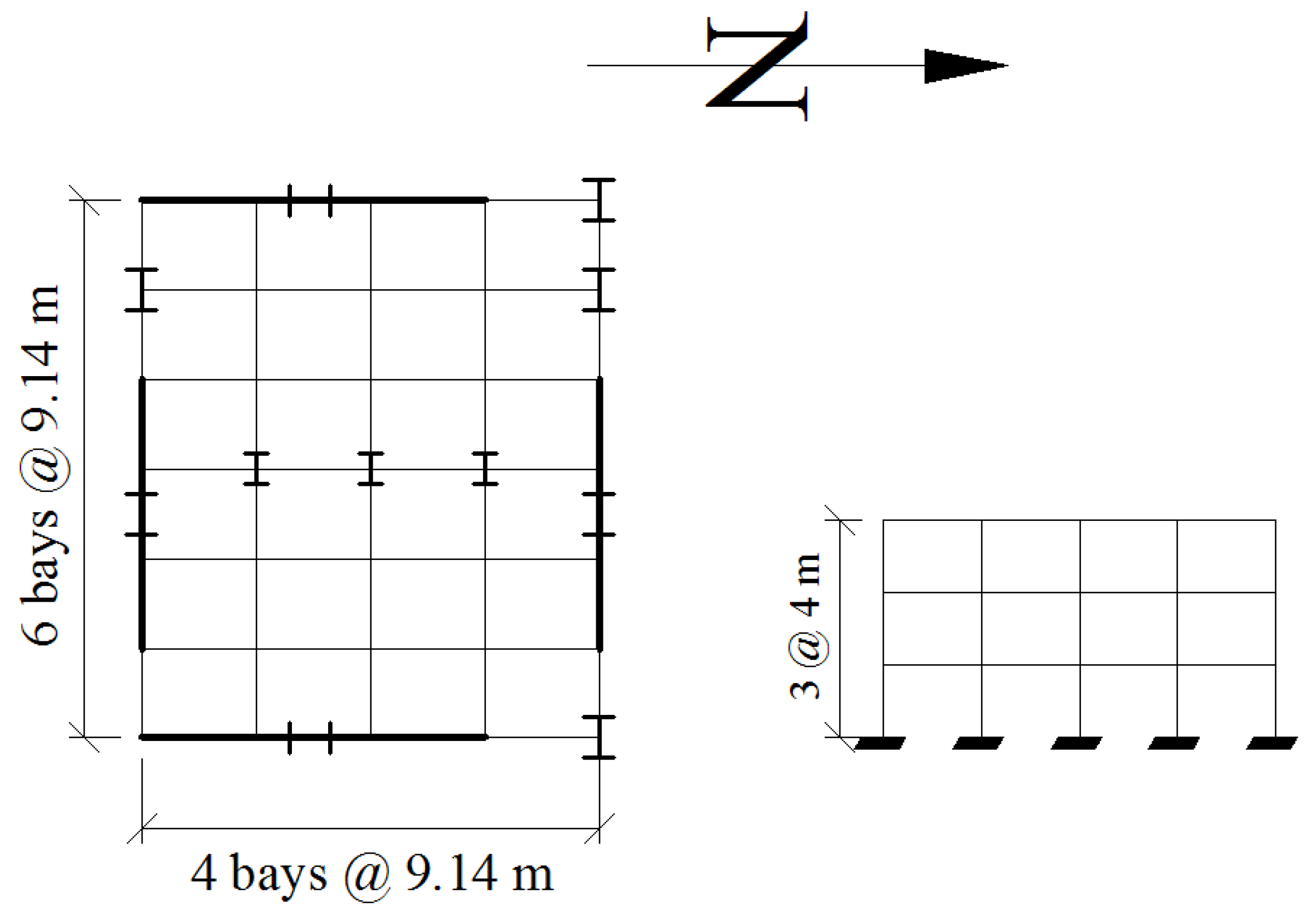
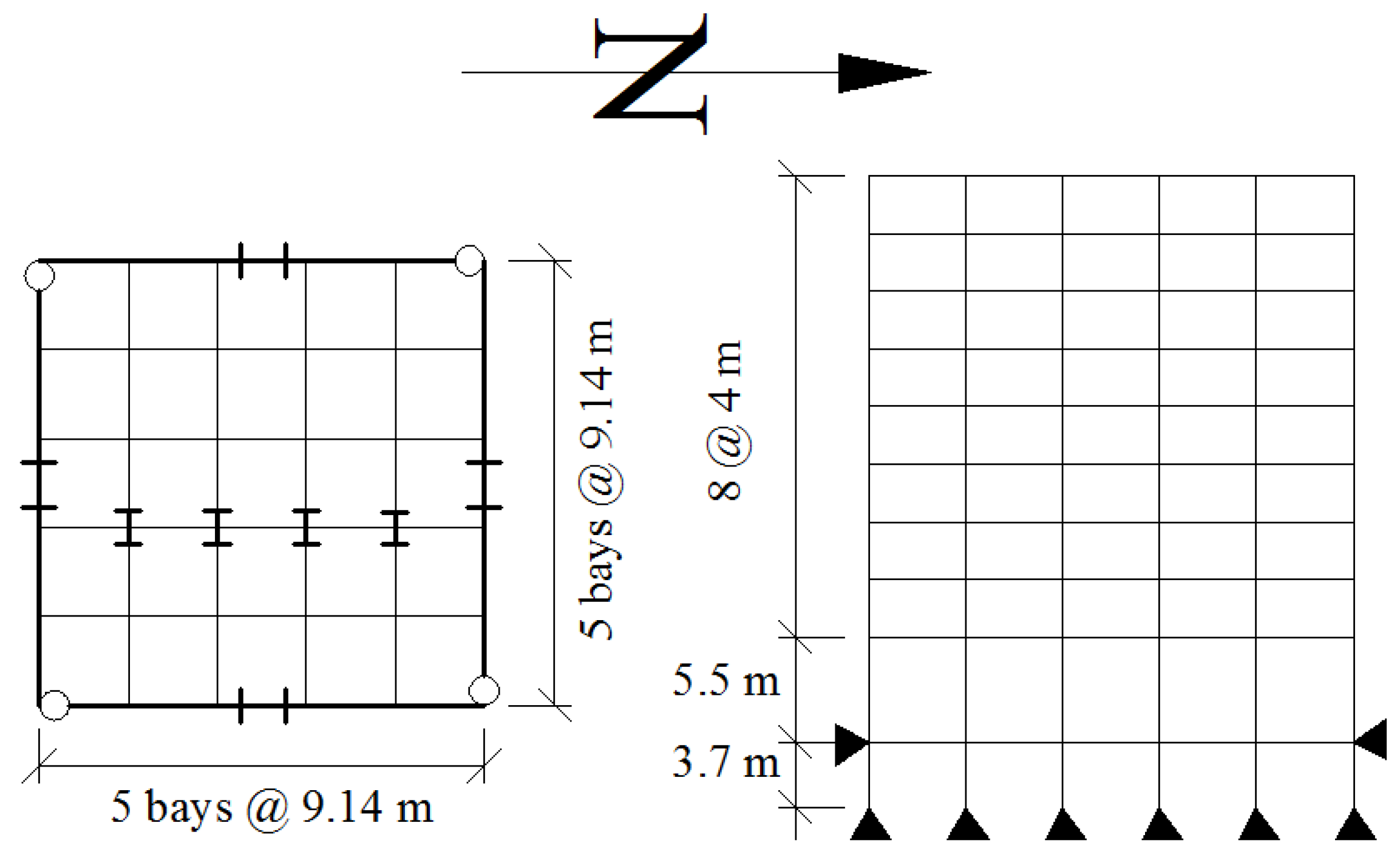
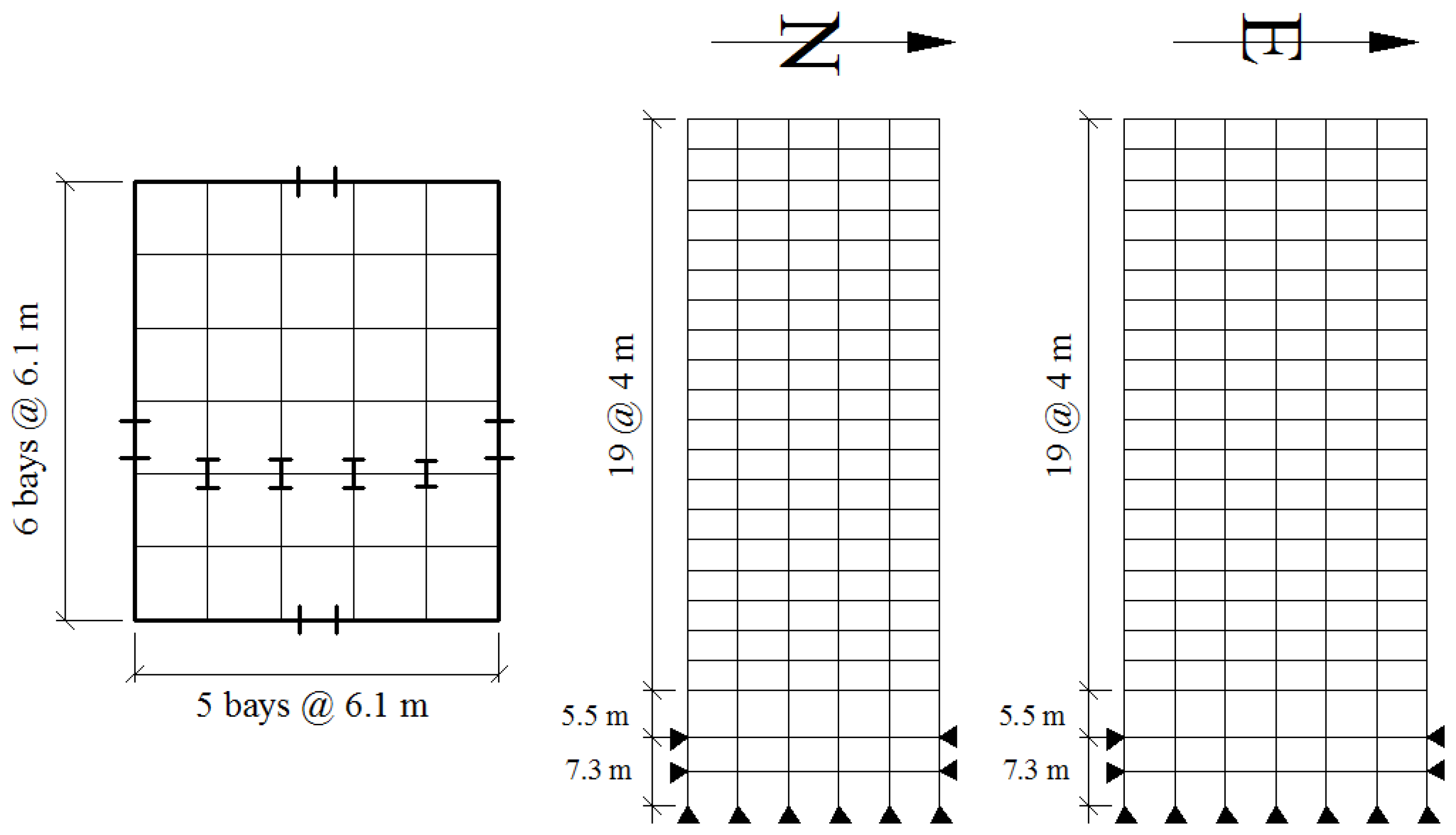
4.1. Structural Models

Three standard 3-, 9-, and 20-story office buildings were selected for the study. These buildings were designed as part of the SAC Steel Project [47] and were assumed to be situated on stiff soil of a high seismic zone. Bi-dimensional (2D) representations of these buildings, which consist of the perimeter moment resisting frames (PMRF), are specifically used as the models of the study. The low-, mid- and high-rise models, which are defined as Models 1, 2 and 3, have fundamental periods of 1.03 s, 2.38 s and 4.07 s, respectively. Some details of the models can be seen in Figure 1, Figure 2 and Figure 3. The structural sections of the vertical and horizontal members can be seen in

Table 1. Wide-flange sections (W-shapes) used in Models 1 and 2.

Model	Story	Columns		Girders
		Exterior	Interior
1	1	14 × 257	14 × 311	33 × 118
	2	14 × 257	14 × 311	30 × 116
	Roof	14 × 257	14 × 311	24 × 68
2	Basement	14 × 370	14 × 500	36 × 160
	1	14 × 370	14 × 500	36 × 160
	2	14 × 370	14 × 500	36 × 160
	3	14 × 370	14 × 455	36 × 135
	4	14 × 370	14 × 455	36 × 135
	5	14 × 283	14 × 370	36 × 135
	6	14 × 283	14 × 370	36 × 135
	7	14 × 257	14 × 283	30 × 99
	8	14 × 257	14 × 283	27 × 84
	Roof	14 × 233	14 × 257	24 × 68

and

Table 2. Wide-flange and box sections used in Model 3.

Story	Columns		Girders
	Exterior	Interior
Basement-1	15 × 15 × 2.00	24 × 335	14 × 22
Basement-2	15 × 15 × 2.00	24 × 335	30 × 99
1	15 × 15 × 2.00	24 × 335	30 × 99
2	15 × 15 × 2.00	24 × 335	30 × 99
3	15 × 15 × 1.25	24 × 335	30 × 99
4	15 × 15 × 1.25	24 × 335	30 × 99
5	15 × 15 × 1.25	24 × 335	30 × 108
6	15 × 15 × 1.00	24 × 229	30 × 108
7	15 × 15 × 1.00	24 × 229	30 × 108
8	15 × 15 × 1.00	24 × 229	30 × 108
9	15 × 15 × 1.00	24 × 229	30 × 108
10	15 × 15 × 1.00	24 × 229	30 × 108
11	15 × 15 × 1.00	24 × 229	30 × 99
12	15 × 15 × 1.00	24 × 192	30 × 99
13	15 × 15 × 1.00	24 × 192	30 × 99
14	15 × 15 × 1.00	24 × 192	30 × 99
15	15 × 15 × 0.75	24 × 131	30 × 99
16	15 × 15 × 0.75	24 × 131	30 × 99
17	15 × 15 × 0.75	24 × 131	27 × 84
18	15 × 15 × 0.75	24 × 117	27 × 84
19	15 × 15 × 0.75	24 × 117	24 × 62
20/Roof	15 × 15 × 0.50	24 × 84	21 × 50

; except for the exterior columns of Model 3, all sections consisted of wide-flange shapes (W-sections). The designation of the structural sections is following the AISC manual [48]. For example, for a W section, the term “14 × 257” corresponds to a W-shape that is nominally 14 in deep and weighs 257 lb/ft. All dimensions of the box sections of Model 3 are in inches. As stated earlier, each building is modeled by a plane MDOF system, where each beam-column is represented by one element. On the other hand, each beam (girder) is represented initially by one element, and then by two and three elements, having nodes at the middle and third of the spans, respectively.

4.2. Earthquake Loading

The seismic records used in this investigation were obtained from the data set of the National Strong Motion Program of the United States Geological Survey (USGS). Fifteen records were selected in such a way that their spectral shape, tectonic regime, magnitude, and fault distance are similar to those controlling the seismic hazard of the area where the buildings are located. It is worth mentioning that the ASCE 7-16 [49] recommends a minimum of eleven pairs of ground motions to take into account the inherent record-to-record variability in the structural response. The main characteristics of such records can be seen in

Table 3. Strong motion records.

Event	Mw	R (km)	PGA (g)		Period (s)		PGV (in/s)
			N-S	E-W	N-S	E-W	N-S	E-W
Imperial Valley, 1940	6.9	10	0.46	0.68	0.53	0.46	12	10
Imperial Valley, 1979	6.5	4.1	0.39	0.49	0.16	0.34	14	11
Landers, 1992 (g)	7.3	36	0.42	0.43	0.73	0.33	7	10
Kern, 1952	7.3	25	0.52	0.36	0.25	0.23	3	3
Loma Prieta, 1989	7	12.4	0.67	0.97	0.21	0.2	9	15
Northridge, 1994, Newhall	6.7	6.7	0.68	0.66	0.31	0.31	9	22
Northridge, 1994, Rinaldi	6.7	7.5	0.53	0.58	0.39	0.29	58	29
Northridge, 1994, Sylmar	6.7	6.4	0.57	0.82	0.31	0.36	36	35
North Palm Springs, 1986	6	6.7	1.02	0.99	0.17	0.21	8	22
Coyote Lake, 1979	5.7	8.8	0.59	0.33	0.15	0.21	8	5
Morgan Hill, 1984	6.2	15	0.32	0.55	0.18	0.16	7	8
Parkfield, 1966, Cholame 5W	6.1	3.7	0.78	0.63	0.37	0.3	4	4
Parkfield, 1966, Cholame 8W	6.1	8	0.69	0.79	0.17	0.21	3	3
North Palm Springs, 1986	6	9.6	0.52	0.38	0.13	0.21	11	26
Whittier, 1987	6	3.62	0.77	0.48	0.7	0.28	11	11

. It can also be observed from the table that the predominant periods of the strong motions records go from 0.13 to 0.72 s. The structural models are subjected to the simultaneous action of the horizontal seismic component (one at a time) of the records, the vertical component, and the gravity loads.

To obtain different levels of deformation, the ground motions are scaled. This is made according to the geometric mean of spectral acceleration (Sa_avg) which is calculated as the “average” of the pseudo-accelerations (S_a) over a range of periods. The range of periods to calculate (Sa_avg) goes from 0.2 T₁ to 1.6 T₁, with constant increments of 0.01 s, where T₁ is the fundamental period of the model. The values of Sa_avg range from 0.2 g up to 1.4 g with uniform increments of 0.2 g for Model 1, while for Model 2 such a range goes from 0.1 g up to 0.8 g with constant increments of 0.1 g. For the case of Model 3, the range of variation of Sa_avg goes from 0.05 g to 0.35 g with constant increments of 0.05 g. It is important to clarify that the maximum values of Sa_avg were chosen in such a way that a similar magnitude of the maximum inelastic deformation, were developed in the three models (drifts of about 3.5%).

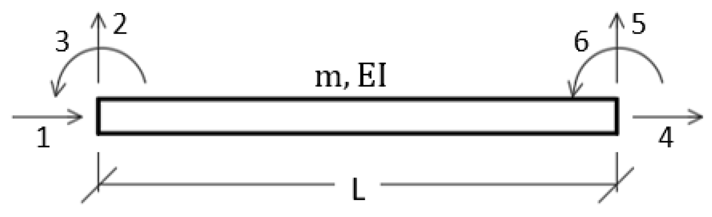
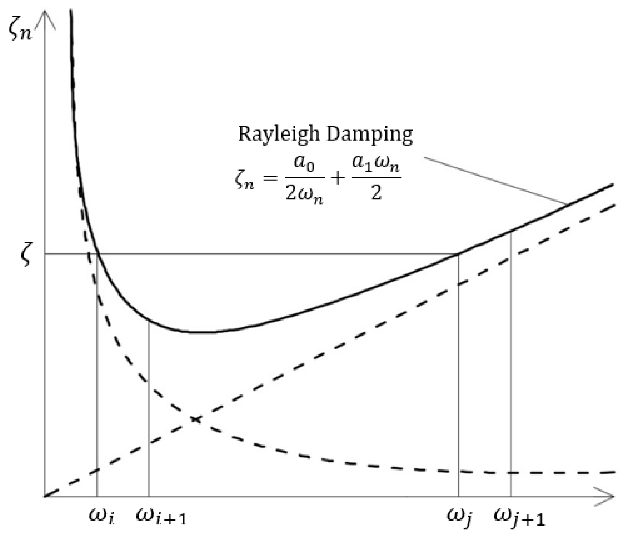
4.3. M and C Matrices

In the analysis of a steel building structure, the mass matrix is commonly obtained by assuming that the mass is concentrated at the nodes. Figure 4 shows the degrees of freedom associated to translations and rotations of a prismatic member with straight axes of a plane steel frame, while Equation (1) illustrates the corresponding mass matrix for an individual element (M_LE). In such an equation, $\overline{m}$ and L represent the mass and the member length, respectively.

$$M_{LE}=\frac{\overline{m}L}{2}\left[\begin{array}{cc}\begin{array}{ccc}1& 0& 0\\ 0& 1& 0\\ 0& 0& 0\end{array}& \begin{array}{ccc}0& 0& 0\\ 0& 0& 0\\ 0& 0& 0\end{array}\\ \begin{array}{ccc}0& 0& 0\\ 0& 0& 0\\ 0& 0& 0\end{array}& \begin{array}{ccc}1& 0& 0\\ 0& 1& 0\\ 0& 0& 0\end{array}\end{array}\right]$$

(1)

It must be noted that the nonzero values are associated to the DOFs 1, 2, 4 and 5 shown in Figure 4, which correspond to translational DOFs. The subscripts L and E in the symbol M_LE stand for the terms lumped and element, respectively.

It is known that the consistent-type mass matrix is more appropriate than the concentrated-type one because the rotational effects [50,51] are considered in the former. By using the d’Alembert´s principle, the virtual work concept and the appropriate interpolation functions, together with the Finite Element Method, it is shown that the element consistent mass matrix (M_CE) is:

$$M_{CE}=\frac{mL}{420}\left[\begin{array}{cc}\begin{array}{ccc}140& 0& 0\\ 0& 156& 22L\\ 0& 22L& 4L^2\end{array}& \begin{array}{ccc}70& 0& 0\\ 0& 54& -3L\\ 0& 13L& -3L^2\end{array}\\ \begin{array}{ccc} 70& 0& 0\\ 0& 54& 13L\\ 0& -13L& -3L^2\end{array}& \begin{array}{ccc}140& 0& 0\\ 0& 156& -22L\\ 0& -22L& 4L^2\end{array}\end{array}\right]$$

(2)

Rayleigh damping model is expressed by Equation (3). In such an equation a₀ and a₁ are proportionality constants that are obtained by fixing modal damping ratios at two modes, namely the i (${\zeta }_i$) and j (${\zeta }_j$) modes. The damping ratio for the n mode is defined as shown in Figure 5, where ω_n is the vibration frequency of that mode. It can be seen (Figure 5) that very large amounts of damping can result in the higher modes. It is argued [44,50,51] that if the i and j modes are adequately selected, the higher mode contribution will be effectively removed because of the very large amounts of damping; however, nothing is stated concerning the resulting very large damping forces. Results of using several combinations of the M (M_L and/or M_C) and K (K_o and/or K_t) matrices in Equation (3) can be found in the literature [3,34,40,41].

$$C=a_{0}M+a_{1}K$$

(3)

The K_t matrix is considered in Equation (3) in this paper. Although it may present some inconveniences, it gives more accurate results than K_o for the following reasons:

(a)

if K_o is used, the elements of the C matrix will not change as the structure behaves inelastically (reducing its stiffness),

(b)

The implication of this is that the fractions of critical damping will increase [43].

(c)

The use of the K_t matrix has been incorrectly criticized due to the fact that when the structure behaves inelastically one did not expect a reduction of damping, but an increment due to the nonlinear behavior. However, such extra damping is considered by the hysteretic behavior of the material.

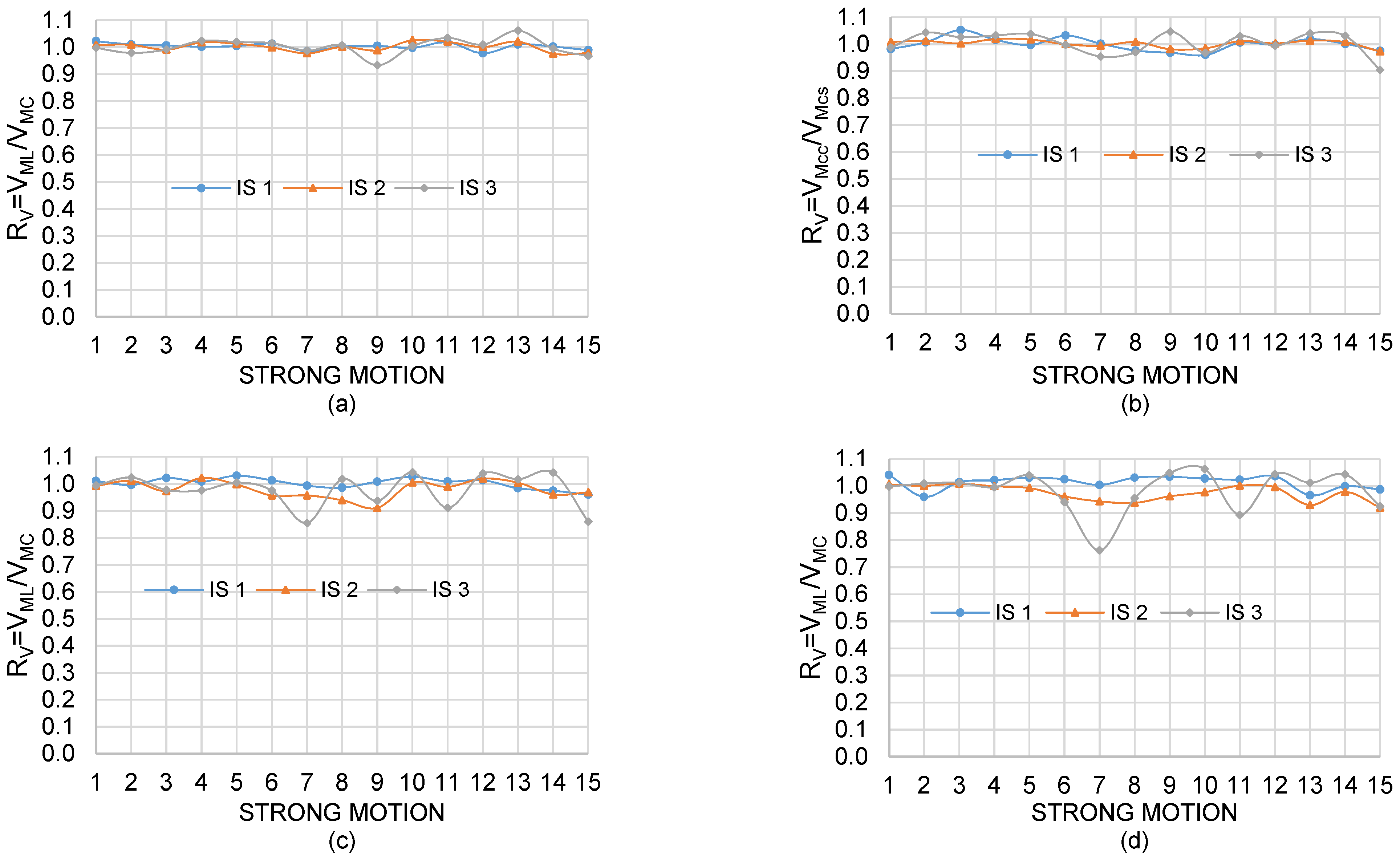
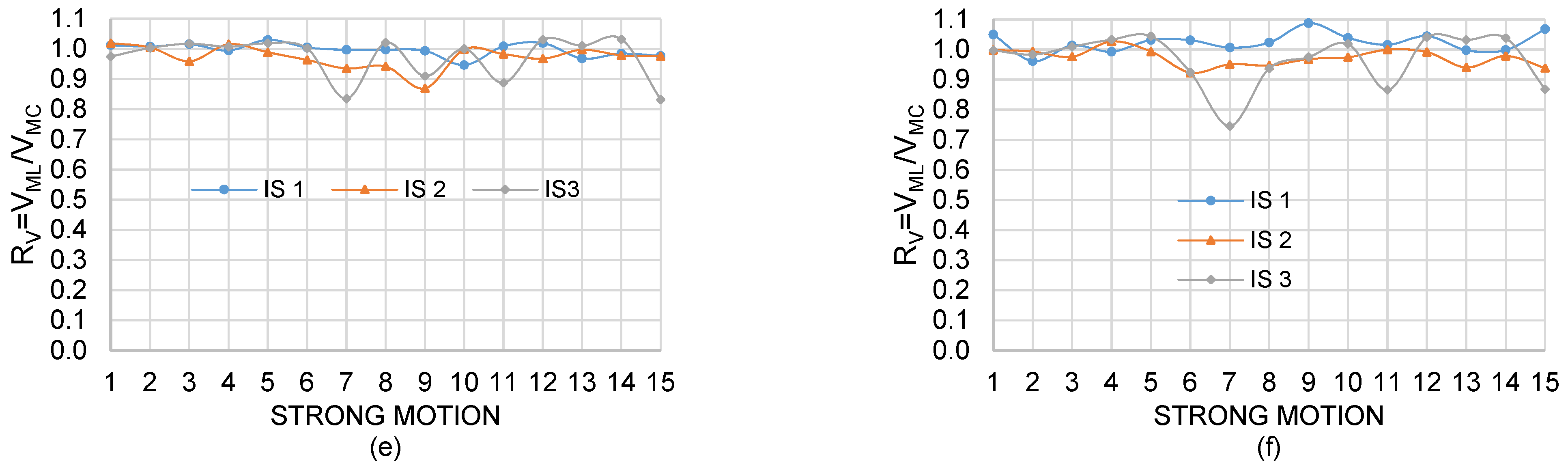
5. Concentrated vs. Consistent Mass

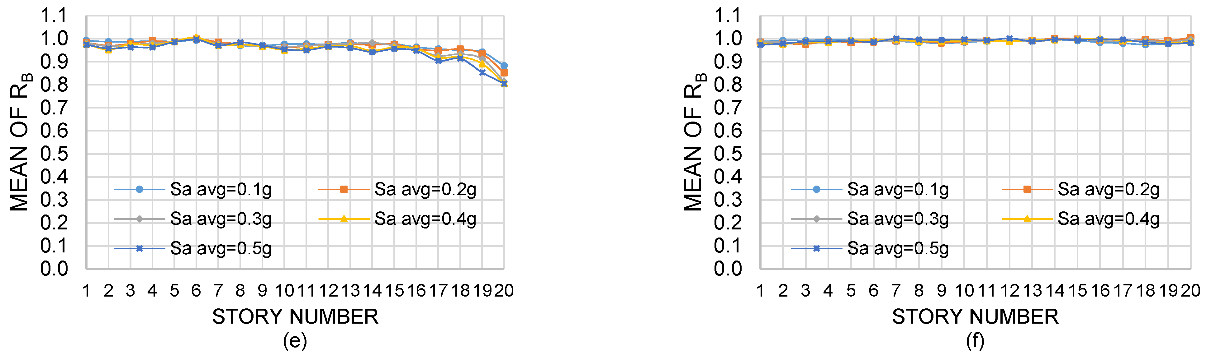
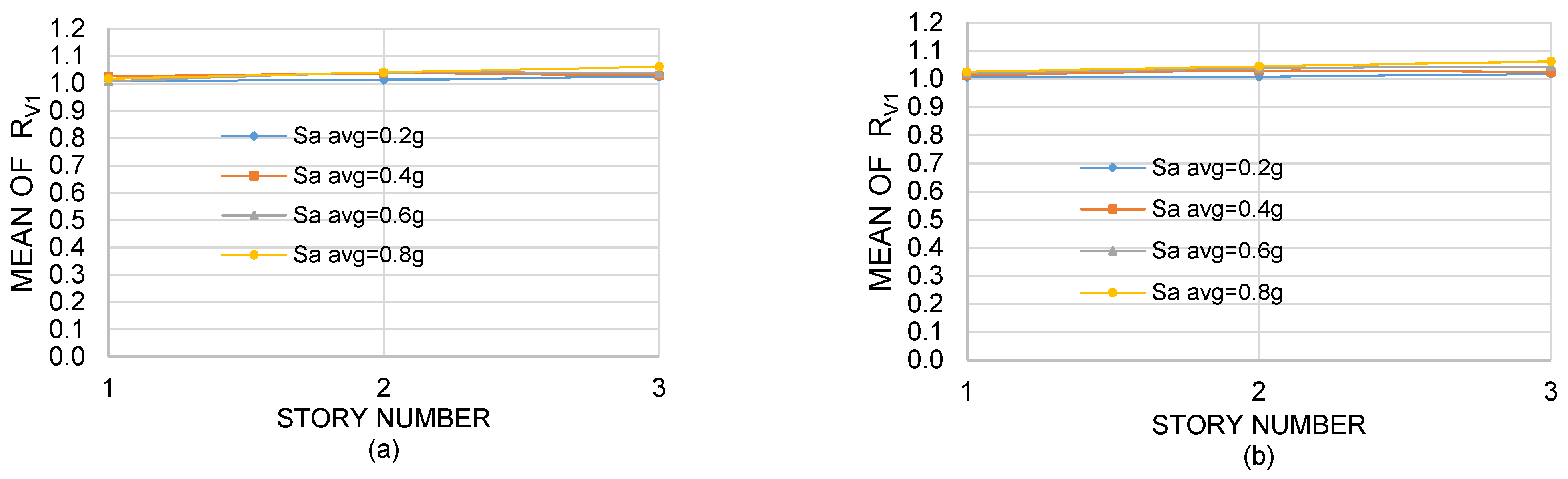
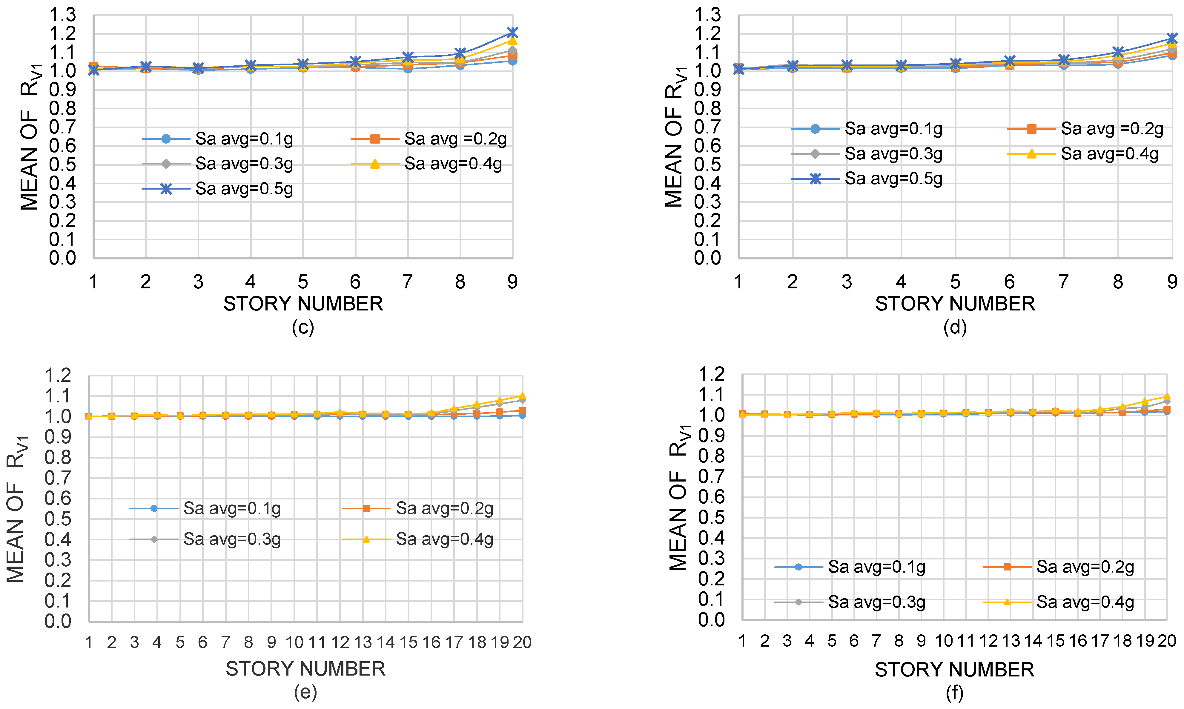
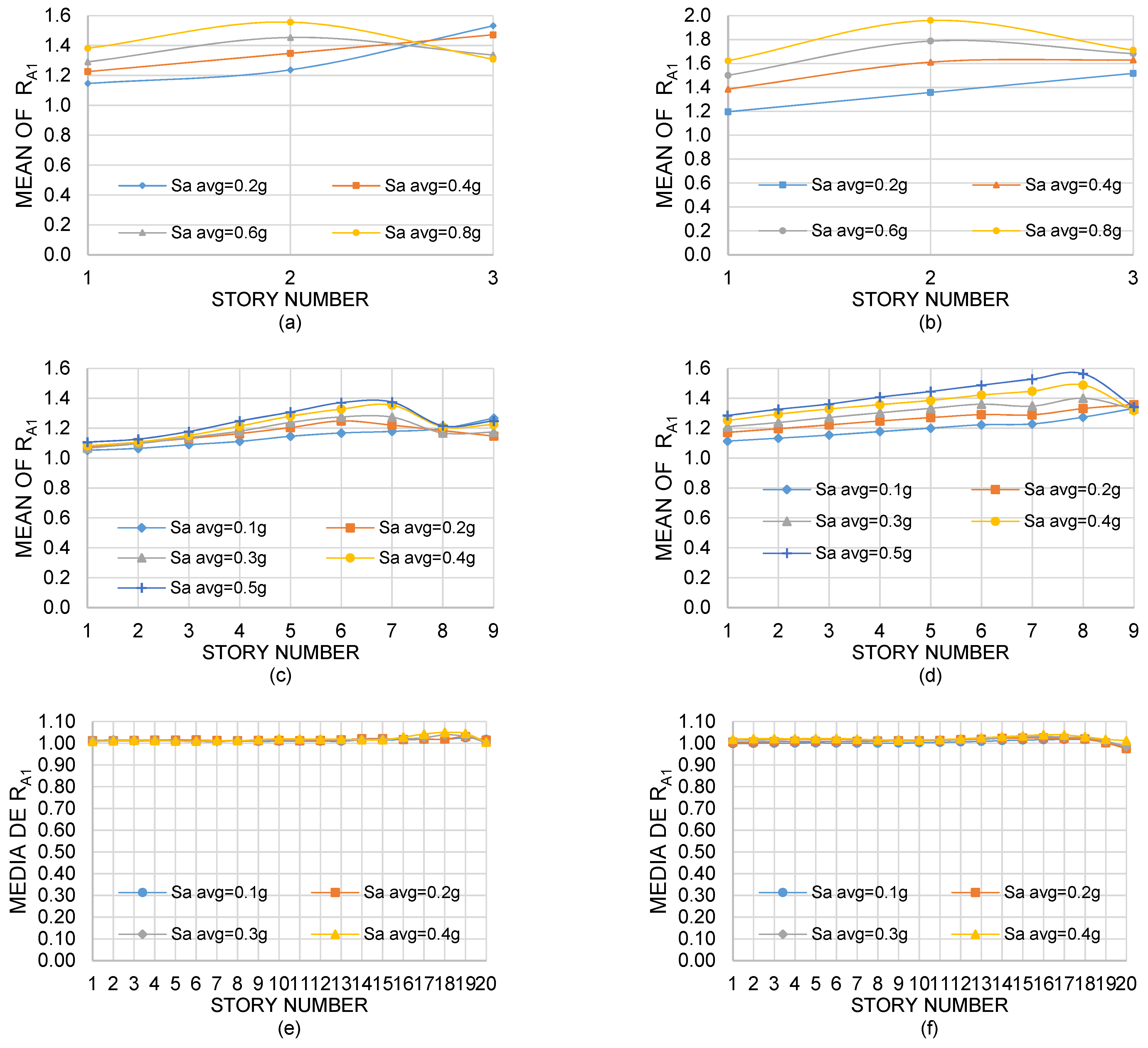
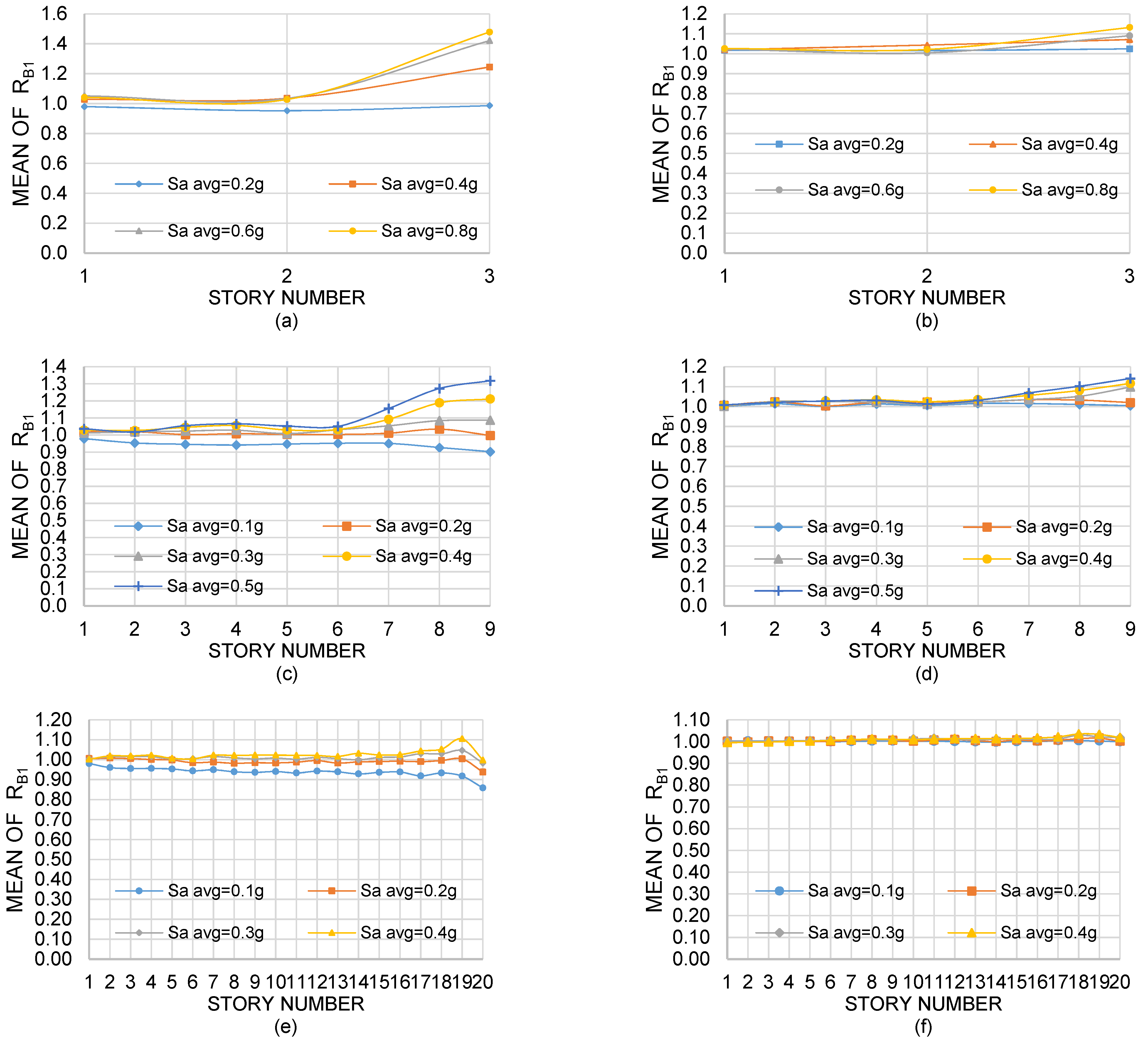
5.1. Comparison for Global Parameters

Global response parameters, i.e., inter-story shears and lateral drifts, are estimated for each story, structural model, direction, strong motion, and seismic intensity, by considering that the mass distribution in the structure is given by the M_L matrix and are compared to the corresponding responses obtained for the M_C matrix. Before presenting the comparison, it is worth mentioning that, considering only the lateral periods of vibrations, the first and second periods are quite similar for the M_C and M_L matrices for the case of Model 1. The third period, in contrast, is 28% greater for M_C. For Model 2, the first five periods are essentially the same for the M_L and M_C matrices, but for modes 6 to 9, they resulted to be larger for the case of M_C, with the differences ranging between 5% and 16%. Similarly, for Model 3, the periods are quite similar for modes 1 through 11 for both types of matrices, but for modes 12 to 20 they are larger for M_C; varying the differences between 6 and 16%.

Results for inter-story shears are compared first. To get this purpose the R_V parameter is used which is defined as

$$R_V=\frac{V_{ML}}{V_{MC}}$$

(4)

where, for a given inter-story, building and strong motion, V_ML and V_MC are the inter-story shears corresponding to the lumped and consistent matrices, respectively.

The values of the R_V ratio for the NS direction of Model 1 are presented in Figure 6a,c,e for seismic intensities of 0.2 g, 0.6 g and 0.8 g, which correspond to small deformations (elastic behavior), moderate yielding, and significant yielding, respectively. The R_V values for the other horizontal (EW) direction are given in Figure 6b,d,f. The term IS abbreviates the expression inter-story. It can be seen from such figures that, if the structure remains elastic (Figure 6a,b), the values of R_V are very close to unity implying that the inter-story shears are essentially the same regardless of the mass matrix model. For moderate and significant yielding, however, values smaller than unity can be seen in many cases implying that the magnitude of the shears is underestimated when the M_L is used. Values of about 0.75 can be seen for some individual seismic records implying underestimations of 25%. The underestimation of R_V seems to increase as one moves up the frame. The values of R_V smaller than unity are due to the fact that the higher- mode contribution, which increases as one moves up the model, is larger for the case of the M_C matrix model.

Despite the strong motions were normalized according to the Sa_avg intensity measure, a considerable dispersion is observed, specifically for large seismic intensities and inter-stories 2 and 3, which reflects, as stated in traditional structural dynamics textbooks [44,50,51], the influence of the inherent variability of seismic records on the response of structures, in addition to that of higher mode contribution.

Plots for the R_V parameter, similar to those shown in Figure 6, were also developed for other seismic intensities for the case of Model 1. Including those of Figure 6, a total of 10 plots were developed for this model. In the same manner, sets of plots of R_V were developed for Models 2 and 3, but they are shown either, only the mean values are presented in all cases; they are shown in Figure 7. Results illustrate that, although for Model 1 underestimations of up to 25% were observed for inter-story shears for some strong motions when M_L is used, on an average basis the underestimation is negligible (about 4%).

For Model 2, average underestimations of up to about 14% can be seen. It is worth mentioning that (even though it is not shown), underestimations greater than 30% occurred for some individual seismic records motions. The corresponding values for Model 3 are about 12% (average) and 26% (individual). It is noted that the results are very similar for the NS and EW directions. It is also observed from Figure 7 that, for a given model, the underestimation increases as the story number increases. The explanation for this is that the contributions of the higher modes for shears at the upper stories are more important for the case of the consistent mass matrix. This higher-mode effect could be expected to be larger for Model 3 than for Model 2. However, the relative plasticization of Model 3, as well as the rotational inertia effects of their beams, are less significant than those of Model 2.

As for inter-story shears, results in terms of drifts were also calculated and compared, but the results are not presented. However, it is worth mentioning that level of underestimation of drifts is smaller than that of shears; the maximum underestimation for individual seismic records is about 9% and in terms of mean values it is about 2%.

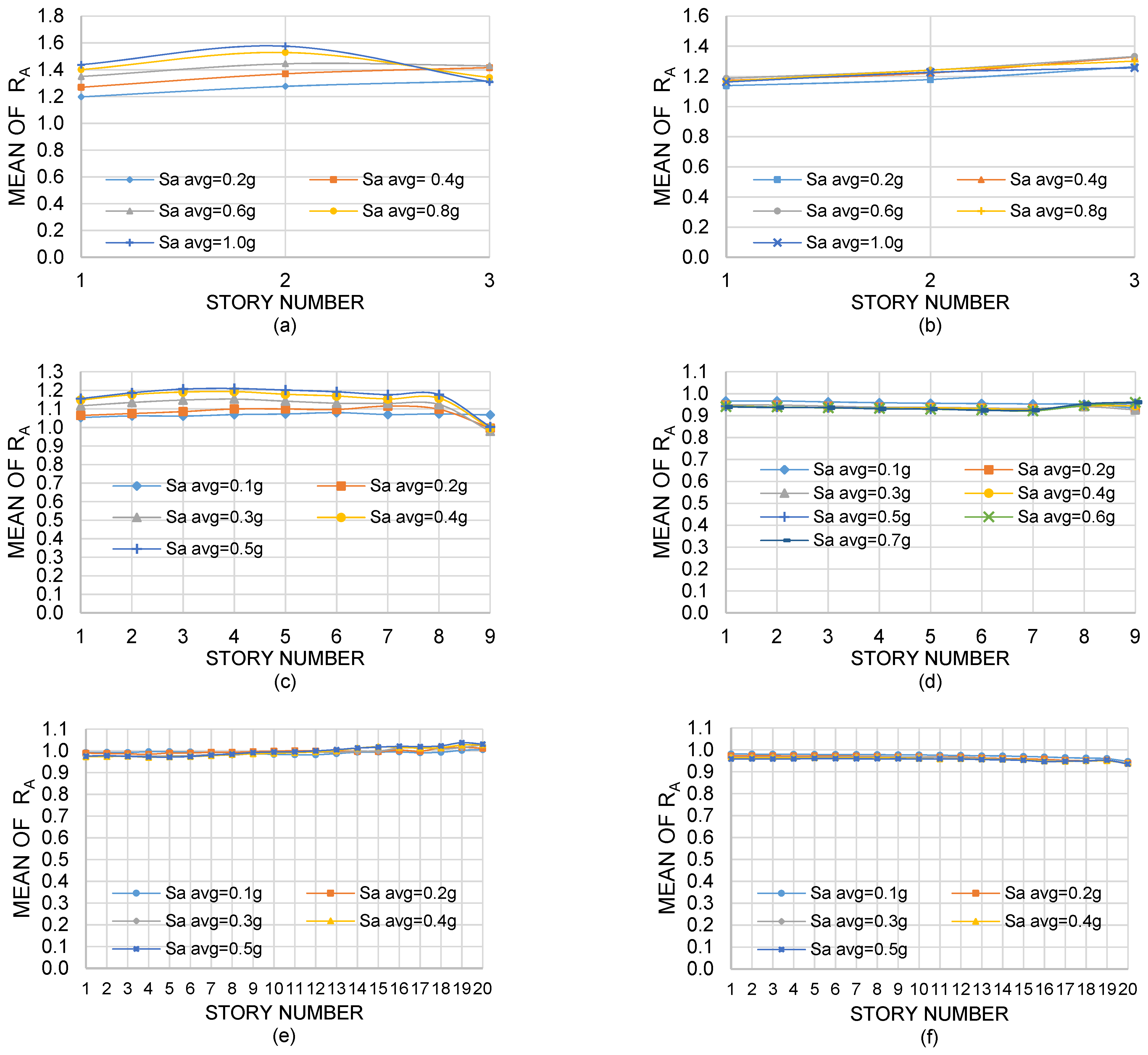
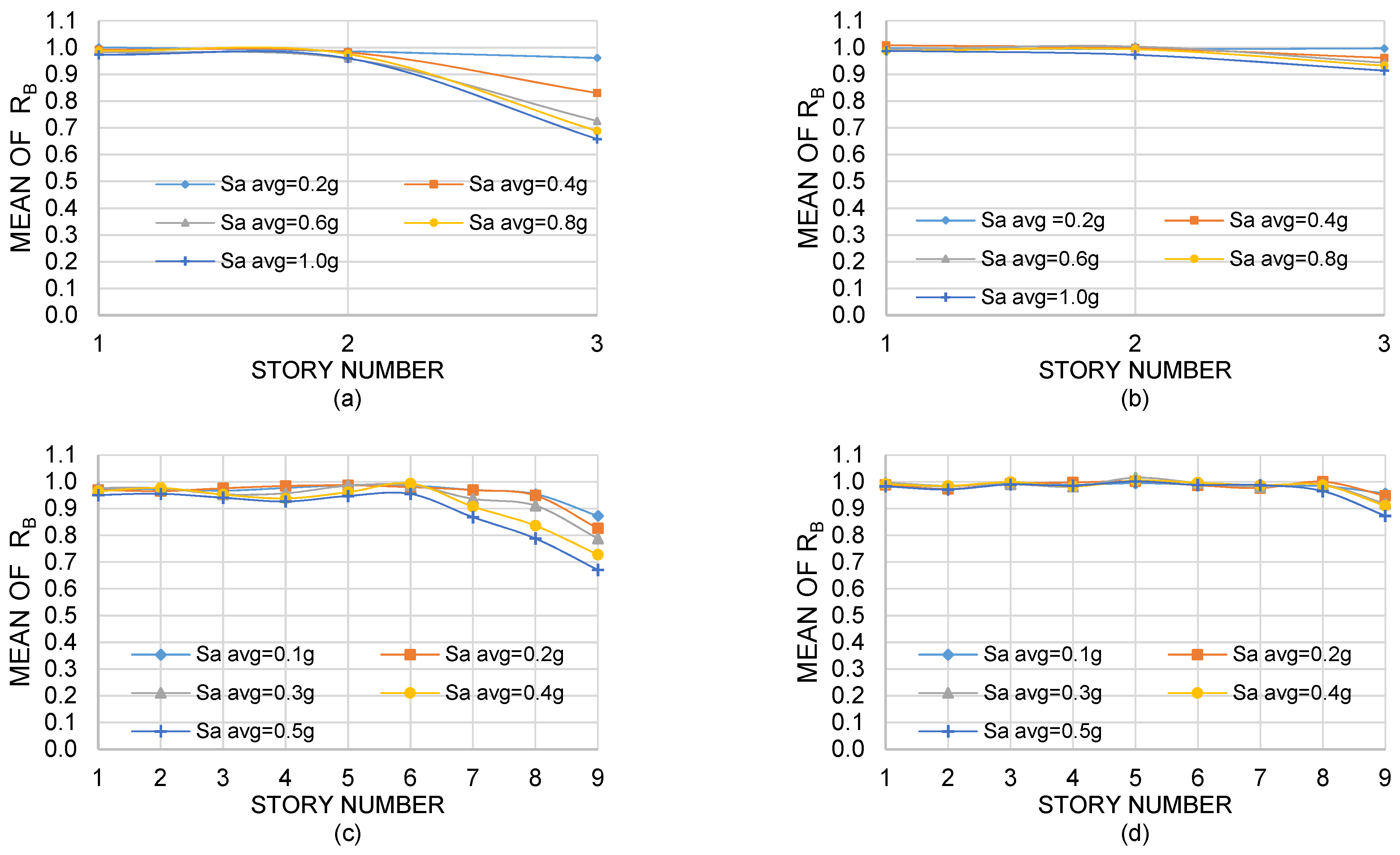
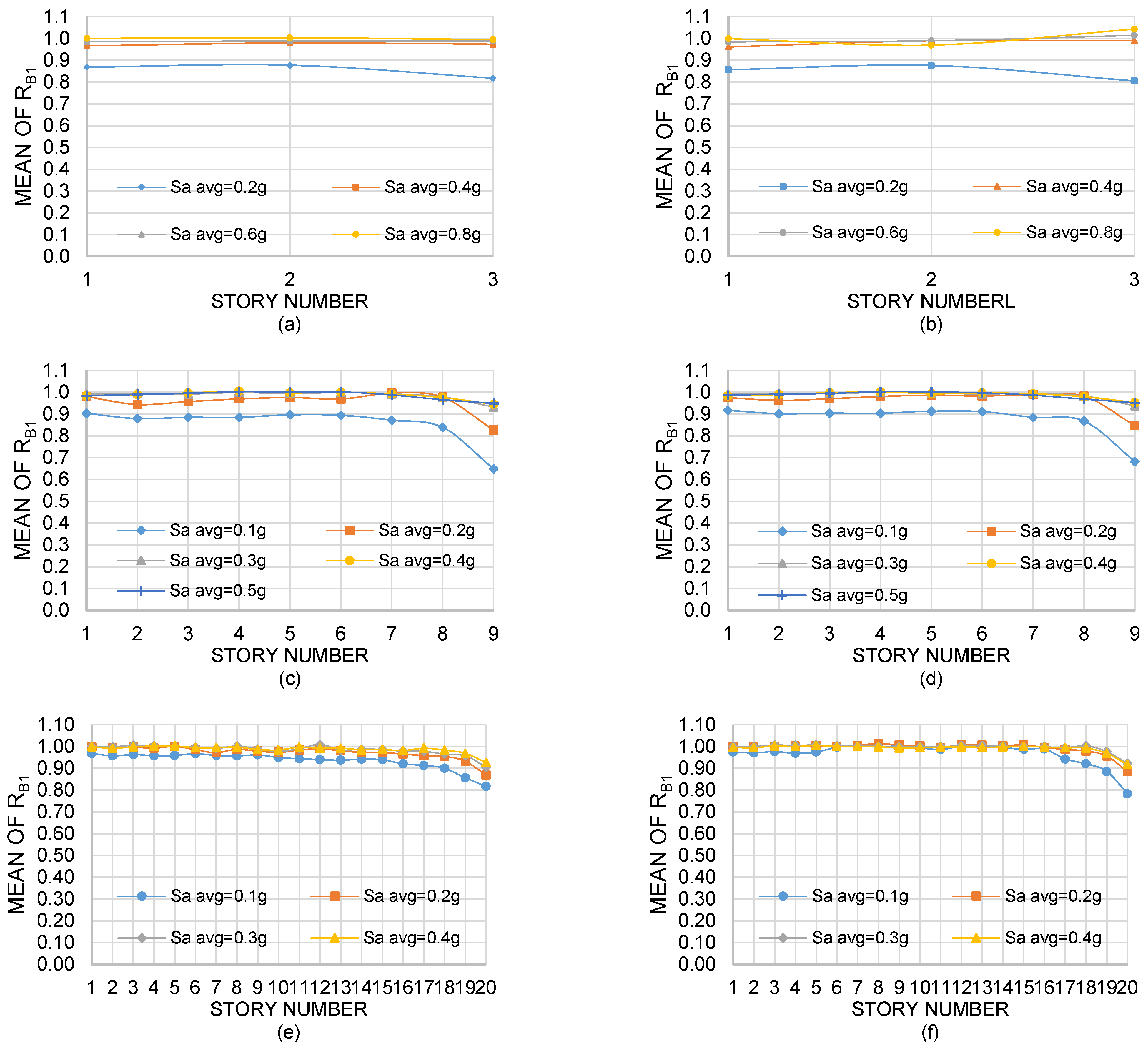
5.2. Comparison for Local Parameters

The axial loads and flexural moments acting on the members of the models with the lumped mass matrix are now compared with the corresponding ones from the consistent mass matrix. For axial loads, the comparison is made for interior and exterior columns, whereas for the case of flexural moments, in addition to columns, a comparison is also made for interior and exterior beams, from the base up to the top. The ratios R_A and R_B given by Equations (5) and (6) are used to make the comparison for axial loads and flexural moments, respectively.

$$R_A=\frac{A_{ML}}{A_{MC}}$$

(5)

$$R_B=\frac{B_{ML}}{B_{MC}}$$

(6)

In the earlier equations, the symbols A and B stand for axial and bending, respectively, so, similar to the R_V ratio, A_ML for example, represents the axial load demands on the frames when M_L is used. Since the results are quite similar for both horizontal directions, the discussion is mainly centered on those of the NS direction. In addition, only the mean values are presented.

The axial loads are compared first. The R_A mean values for exterior columns can be seen in Figure 8a,c,e, for Models 1, 2 and 3, respectively, while the corresponding mean values for the interior ones are given in Figure 8b,d,f. It can be seen that, for exterior columns, unlike shears and displacements, the R_A mean values are in many cases significantly larger than unity implying that the axial loads on these structural members can be considerably overestimated if the M_L model is used. Values of up to 1.6 can be seen for inter-story 2 of Model 1 implying, on an average basis overestimations of up to 60%. Even for elastic structural behavior (Sa_avg = 0.2 g) R_A mean values of about 1.3 can be observed. Overestimation larger than 100% (not shown) occurred for individual seismic records. Excepting the last inter-story of the 3- and 9-story models, the values increase as Sa_avg increases; however, they tend to decrease with the building height, so for the tallest model the maximum level of overestimation is observed to be about 5%.

There are many considerable differences in the responses for interior columns with respect to those of exterior columns. The axial loads on interior columns of the 3-story model, the individual, and average underestimations are up to 44% and 30%, respectively. The corresponding values for the interior columns of the 9- and 20-story models are about 18% and 8%. One of the reasons for this is that, for a given floor, the interaction between beams and exterior columns is expected to be very different from that of the interiors, since the former are connected to columns only at one end, while the latter are connected at both ends.

The mean values of R_B for the NS direction, for all columns and models, are shown in Figure 9. It is observed that for exterior columns (Figure 9a,c,e) the flexural moments may be considerably underestimated when M_L is used. The amounts of underestimation increase as Sa_avg and the story number increase; in contrast, they tend to decrease as the model becomes taller. The maximum values are about 0.65, 0.68 and 0.80, indicating average underestimations of 35%, 32% and 20%, for Model 1, 2 and 3, respectively. Considering individual seismic records, the corresponding maximum levels of underestimation are about 66%, 58% and 42%. As for axial loads, the underestimation of flexural moments on interior columns is less significant than that of the exteriors; for Models 1 and 2 the maximum individual and average underestimations are around 21% and 11%, respectively; for Model 3, on the other hand, the flexural moments are essentially the same for M_L and M_C.

The mean values of R_B for exterior and exterior beams were also calculated, but the results are not presented. It is worth mentioning, however, that the level of underestimation is much smaller than that of interior columns. The flexural moments of the models with M_L were also compared to those of M_C, for the case of exterior and interior beams but, the results are not presented. It is important to mention, however, that underestimation is less significant even than that of interior columns.

The earlier results indicate that the effect of the mass matrix model can significantly vary from one parameter to another. There are many reasons for this; axial loads for example are directly affected by the vertical modes of vibration, which is not the case for interstory shears. Another reason is that due to the fact that the numerical values of the elements of the M_L matrix associated to vertical vibration are greater than those of the M_C matrix, the larger inertial vertical effects, and consequently larger axial loads on columns, are expected for the case of M_L. For the case of bending moments the opposite occurs, that is, the bending moments are larger for the M_C matrix because the rotational inertias are larger in comparison with those of the M_L matrix. The overestimation tends to increase as one moves up the model, since the contribution of the higher-mode response may have enhanced for the case of the M_C matrix.

In summary, depending upon the response parameter under consideration, the structural model, the seismic intensity and the structural location, the responses can be precisely calculated, considerably overestimated, or considerably underestimated when M_L is used. The inter-story shears, on an average basis, are underestimated by up to about 15%, but for individual strong motions they are underestimated by up to 30%. It can be said that the underestimation is negligible for lateral drifts. The axial loads at exterior columns are significantly overestimated by up to 100% and 60% for individual strong motions and on an average basis, respectively; the corresponding values for the interiors are 44% and 30%. Flexural moments at exterior columns may be underestimated by up to 60% and 35%, individually and on average, respectively; the corresponding values for interior columns are about 21% and 11%. On the other hand, there is no error in the estimation of flexural moments at beams if M_L is used.

Structural members in MRFs are designed as beams or beam-columns. In traditional seismic design procedures of steel buildings around the world [48], the members are first designed following the strength concept and then the drifts are revised. It is shown in this paper that there are no significant errors in drifts if the M_L matrix is assumed in the analysis. For inter-story shears and flexural moments, on the other hand, significant non-conservative errors may result in the design. Hence, it is strongly suggested to use the M_L model while numerically modeling the structural system (steel MRFs) considered in the study.

One of the main justifications in the past to avoid the use of the consistent mass matrix was the greater computation (implying greater cost) time demand. However, these days this justification is no longer valid; using modern computers together with efficient modern operating systems, the differences between the computer time requirements of the concentrated and the consistent mass matrices are tremendously reduced.

6. One vs. More than One Element per Member

It was commented in Section 1 that in typical seismic analysis of steel frames, the common practice is to use only one element per member (no intermediate nodes), including for the beams. In this section of the paper, the precision of using this practice is quantified. The consistent mass matrix is assumed in these analyses. To this aim, the same response parameters studied in Section 5 are considered, but now discretizing the beams by using one, or two, intermediate nodes; the responses are compared to those obtained without considering intermediate nodes. It is important to mention that some periods, associated to lateral vibration, are significantly modified when intermediate nodes are used in the beams. For the 3-story frame, by example, the first period is essentially the same for the model with and without one intermediate node. The periods for modes 2 and 3, on the other hand, increase 10% and 98%, respectively. For the 9-story model, no increments occur in the periods of modes 1 through 4, but for modes 5 to 9 increments, which range from 28% to 35%, are observed. For the 20-story model, there are no changes for the first eleven periods, but significant increments occur for the remaining nine lateral modes, which range from 11% to 21% if one intermediate node is used.

It is assumed that the greater the number of elements per member, the better the seismic response since the distribution of mass is more uniform. In the subsequent discussion, the abbreviations 1E, 2E and 3E will symbolize the structural models obtained from considering one, two and three elements per beam, respectively.

6.1. Global Response Parameters, Two Elements per Beam (2E)

To make the comparison for inter-story shears, the parameter R_V1, defined by Equation (7) is used. In such an equation, V₁ and V₂ symbolize the shears for models 1E and 2E, respectively. As in many other discussions, only the results of R_V1, averaged over all the seismic records, are shown.

$$R_{V1}=\frac{V_1}{V_2}$$

(7)

Figure 10 illustrates the mean values of R_V1 for all the models. It can be seen that, on an average basis, the values essentially equal unity for the 3-story building, implying that there are no differences between the shears of Model 1E and those of Model 2E. For the 9-story model, in contrast, the average R_V1 values significantly increase with respect to those of the 3-story model. The values increase through the height of the model; the largest observed value is 1.21 implying that the shears can be overestimated by up to 21% if just one element per beam is used in the structural modeling. For the case of the taller model (Model 3), the average values of R_V1, similar to those of Model 2, in general increase through the height of the model, but the values, although still significant, are smaller than those of Model 2, the maximum average value is observed to be 1.10. Even though they are not shown, overestimations of up to 33% can be seen individually for some seismic records.

The responses for lateral drifts are also calculated and contrasted for the 1E and 2E structural representations. The parameter used to make the comparison is R_D1, but the results are not shown. It is mentioned, however, that the average values of R_D1 are essentially equal to unity for any model and seismic intensity indicating that the lateral drifts are precisely calculated if one element per beam is considered.

6.2. Local Response Parameters, Two Elements per Beam (2E)

To compare the axial loads on the columns of Models 1E with those of Model 2E, the R_A1 ratio, defined by Equation (8), is used. The numerator and denominator in such an equation have the same meaning as those of Equation (7), but now axial loads in columns are analyzed instead.

$$R_{A1}=\frac{A_1}{A_2}$$

(8)

The average of the R_A1 values for the exterior columns as well as for the interiors are presented in Figure 11 for all the models. Only the results for the NS direction are presented. Results from the figure indicate that, unlike the case of shears and drifts, axial loads on columns may be significantly overestimated when one element per beam is considered. For a given model the magnitude of the overestimation increases as the story number and the seismic intensity increase, but it decreases as the model becomes taller. The average overestimations can be up to 95%, 55% and 5%, for Models 1, 2 and 3, respectively; the corresponding maximum overestimations considering individual seismic records can be up to 140%, 86%, and 13%. Even for the case of elastic behavior, significant overestimations can be seen for the case of the 3-, and 9-story models.

The R_B1 ratio given by Equation (9) is used to compare the seismic responses in terms of flexural moments. Similar to the R_V1 and R_A1 parameters, B₁ and B₂ represent the flexural moments at columns for the 1E and 2E structural representations.

$$R_{B1}=\frac{B_1}{B_2}$$

(9)

The R_B1 averages for exterior columns as well as for the interiors are shown in Figure 12. As for the R_A1 parameter, the results are similar for the two horizontal directions; consequently, only the values associated to the NS direction are presented. The mean values of R_B1 resemble those of R_A1 in the sense that, for the case of significant structural deformations, the flexural moments of exterior columns may be significantly overestimated when no intermediate node is used, with the level of overestimation decreasing with the height of the model. The maximum overestimations (on average) are 48%, 32%, 11%, and for Models 1, 2 and 3, respectively; however, considering individual seismic records, the corresponding maximum overestimations are 68%, 59%, and 19%. For the lowest structural deformations, on the other hand, the flexural moments can be underestimated; on an average and individual basis, the maximum overestimations can be up to 12%, 24%, 29% and 5%, 10%, 14%, respectively. It is observed that the overestimation is much smaller for the case of interior columns.

The R_B1 averages for interior beams, as well as for the interiors, are presented in Figure 13 for all the models. It is seen that for elastic behavior (smallest values of Sa_avg), the flexural moments at both, exterior and interior beams are underestimated; the level of underestimation increases with the story number; the observed amounts of individual and average underestimation are about 38%, 60%, 45% and 19%, 35%, 22% for the Models 1, 2 and 3, respectively. For intermediate or large deformations, on the other hand, the values are essentially equal to unity in almost all cases, which implies that the bending moments in the beams without intermediate nodes are very similar to those resulting from the consideration of an intermediate node.

6.3. Global and Local Parameters, 2 Intermediate Nodes

The same parameters analyzed earlier, namely lateral drifts, shears, axial loads, and flexural moments, are now calculated for the representation 3E of the models and contrasted to those of the representation 1E. Ratios of the responses of representation 1E to those of representation 3E of the models were developed. However, since no considerable differences were observed with respect to those of Section 6.1 and Section 6.2 (where 1E and 2E were compared), only a few comparative ratios for the case of local response parameters are presented.

Equations (10) and (11) are used to make the comparison for axial loads and flexural moments, respectively. A₃ and B₃ in these equations represent the axial loads and flexural moments, respectively, in the members when three elements per beam (representation 3E) are used in the models. The other terms were defined earlier.

$$R_{A2}=\frac{A_1}{A_3}$$

(10)

$$R_{B2}=\frac{B_1}{B_3}$$

(11)

The R_A2 averages for exterior columns of Models 1 and 2 are presented in Figure 14a,b, respectively. Most of the major observations made before for the 1E and 2E comparison (Figure 11a,c) apply to this case. However, it is observed that, for the 3-story model, the level of overestimation of axial loads when no intermediate nodes are used resulting from the comparison 1E-3E is a little greater than that of the comparison 1E-2E (68% vs. 56%). For Model 2, on the other hand, the level of overestimation is essentially the same (about 40%) for the two comparison cases.

The average values of R_B2 for exterior columns can be seen in Figure 14c,d. Results indicate that the levels of overestimation, or underestimation, of these flexural moments obtained from the comparison of the 1E and 3E structural representations, essentially remain the same as those of the 1E and 2E representations.

The R_B2 averages of beams are can be seen in Figure 15. By comparing the results with those of Figure 14a through Figure 14d (1E vs. 3E) it is concluded that, as for the case of flexural moments at columns, the level of underestimation in flexural moments of beam obtained from the comparison 1E–2E is quite similar to that of the comparison 1E–3E. The responses of the models with four elements (three intermediate nodes) per beam were also calculated for some cases, but the results are not shown. It is worth mentioning, however, that the results are essentially identical to those of the representation 3E.

The abovementioned results indicate that there is a certain degree of overestimation or underestimation of the seismic response when intermediate nodes are not used in the beams. Such underestimations or overestimations turned out to be practically the same when the results of not considering intermediate nodes were compared with those of one, two, or three intermediate nodes. Hence, there is no necessity of using more than three elements to represent the beams since practically convergence is reached for this number of elements. The accuracy is good even for the two-element case.

From the earlier discussion it is concluded that if just one element per beam is used, the magnitude of inter-story shears can be overestimated by up to 33% and 21% for individual strong motions and on an average basis, respectively. The lateral drifts, however, are essentially the same for the models with none or with intermediate nodes. Considerable overestimations occur for axial loads in columns, including elastic behavior; the maximum overestimations are about 145% and 95% (individually and on average). Flexural moments at exterior columns can also be significantly overestimated for high seismic intensities; the maximum overestimations are about 68% and 48% (individually and on average). On the other hand, for the lowest structural deformations (smaller values of Sa_avg), the flexural moments at columns are underestimated by up to 29% and 14% (individually and on average). The flexural moments at exterior and interior beams are underestimated by up to 60% and 35% individually and on average, respectively. The underestimation (or overestimation) calculated by comparing the responses of the 1E and 2E structural representations is quite similar to that of comparing the responses of the 1E and 3E structural representations, which indicates that convergence is reached in the responses when three elements per beam are considered.

7. Conclusions

The responses of steel moment-resisting frames (MRFs) considering the mass matrix as concentrated (M_L) are calculated and contrasted with those calculated by considering that such matrix is consistent (M_C). The responses are also calculated by considering just one element per beam and are compared with those of assuming two and three elements. Steel frame models, representative of low, medium, and tall steel buildings, modeled as multi-degree-of freedom systems under the action of 15 seismic records, representative of the area of the model locations, are used in the numerical study. The comparison is made in terms of overall parameters (inter-story shear and displacements) as well as in terms of local parameters (axial loads and flexural moments at exterior and interior beams and columns). The main findings are:

1. Depending on the parameter, the structural model, the seismic intensity and the member location, the responses may be precisely calculated, significantly overestimated or underestimated, when M_L is used. The inter-story shears, on an average basis, are underestimated by up to about 15%, but underestimations of up to 30% can be seen for some individual seismic records. The lateral drifts are precisely calculated, but axial loads at columns can be significantly overestimated (up to 60% and 100% on average and individually, respectively). Flexural moments at columns, on the other hand, are underestimated; average and individual underestimations of up to 35% and 60%, respectively, can be seen. The flexural moments at beams are precisely calculated.

2. Inter-story shears can be overestimated if just one element per beam is used in the structural modeling; average and individual overestimation of up to 21% and 33%, respectively, can be seen. The lateral drifts, however, are precisely calculated. For significant deformations, the corresponding amounts of average and individual overestimation for axial loads at columns are about 95% and 140%, while those of flexural moments are 48% and 68%. The flexural moments at columns for the lowest structural deformations, on the other hand, can be underestimated; the maximum amounts of average and individual underestimations are about 14% and 29%, respectively. Underestimations by up to 35% and 60% (on average and individually) are observed for flexural moments at beams for small deformations, but for intermediate and large deformations, they are precisely calculated. The underestimation or overestimation obtained by comparing the responses of the models without intermediate node with those of one intermediate node is quite similar to that of comparing the responses of the models without intermediate nodes with those of two, or three, intermediate nodes; it indicates that convergence is reached in the responses when three elements per beam are considered.

3. Structural members in MRFs are normally designed as beams or beam-columns based on the strength concept to support the member forces; then lateral drifts are revised. The results of this study indicate that the introduced errors for lateral drifts are neglectable if M_L, or one element per beam is used, but significant errors may be introduced in the design due to the overestimation and underestimation of the design forces. For those reasons, it is strongly suggested to use the M_C model and at two elements per beam in the structural modeling.

4. One of the main justifications in the past for not using the consistent mass matrix was the great computation (implying greater cost) time demand. However, these days, this justification is no longer valid at least for buildings modeled as 2D systems; using modern computers together with efficient modern operating systems, the computation time has been significantly reduced and so the differences between the time requirements for the concentrated and the consistent mass matrices, as observed while developing this research.

References

1. Osman, A.; Ghobarah, A.; Korol, R.M. Implications of design philosophies for seismic response of steel moment frames. Earthq. Eng. Struct. Dyn. 1995, 24, 127–143. [Google Scholar] [CrossRef]
2. Li, G.; Li, J. Advanced Analysis and Design of Steel Frames; John Wiley & Sons: Hoboken, NJ, USA, 2007. [Google Scholar]
3. Ozel, H.F.; Saritas, A.; Tasbahji, T. Consistent matrices for steel framed structures with semi-rigid connections accounting for shear deformation and rotary inertia effects. Eng. Struct. 2017, 137, 194–203. [Google Scholar] [CrossRef]
4. European Committee for Standardization. Eurocode 8 EN 1998-1: Design of Structures for Earthquake Resistance, Part 1, General Rules, Seismic Actions and Rules for Buildings; European Committee for Standardization: Brussels, Belgium, 2004. [Google Scholar]
5. International Code Council. International Building Code (IBC); International Code Council: Washington, DC, USA, 2009; ISBN 9781580017428. [Google Scholar]
6. Canadian Commission on Building and Fire Codes. The National Building Code of Canada; National Research Council of Canada: Ottawa, ON, Canada, 2010.
7. Jennings, P.C. Equivalent viscous damping for yielding structures. J. Eng. Mech. Div. ASCE 1968, 94, 103–116. [Google Scholar] [CrossRef]
8. Gulkan, P.; Sozen, M. Inelastic response of reinforced concrete structures to earthquake motions. ACI J. 1974, 71, 604–610. [Google Scholar]
9. Iwan, W.D. Estimating inelastic response spectra from elastic spectra. Earthq. Eng. Struct. Dyn. 1980, 8, 375–388. [Google Scholar] [CrossRef]
10. Hadjian, A.H. A re-evaluation of equivalent linear models for simple yielding systems. Earthq. Eng. Struct. Dyn. 1982, 10, 759–767. [Google Scholar] [CrossRef]
11. Wijesundara, K.K.; Nascimbene, R.; Sullivan, T.J. Equivalent viscous damping for steel concentrically braced frame structures. Bull. Earthq. Eng. 2011, 9, 1535–1558. [Google Scholar] [CrossRef]
12. Weare, W.; Gere, J. Matrix Analysis of Framed Structures; Springer: Berlin/Heidelberg, Germany, 1990. [Google Scholar]
13. Qin, H.; Li, L. Error Caused by Damping Formulating in Multiple Support Excitation Problems. Appl. Sci. 2020, 10, 8180. [Google Scholar] [CrossRef]
14. Yang, P.; Xue, S.; Xie, L.; Cao, M. Damping Estimation of an Eight-Story Steel Building Equipped with Oil Dampers. Appl. Sci. 2020, 10, 8989. [Google Scholar] [CrossRef]
15. Mohamed, O.; Khattab, R. Assessment of Progressive Collapse Resistance of Steel Structures with Moment Resisting Frames. Buildings 2019, 9, 19. [Google Scholar] [CrossRef] [Green Version]
16. Shehu, R.; Angjeliu, G.; Bilgin, H. A Simple Approach for the Design of Ductile Earthquake-Resisting Frame Structures Counting for P-Delta Effect. Buildings 2019, 9, 216. [Google Scholar] [CrossRef] [Green Version]
17. Archer, J.S. Consistent matrix formulations for structural analysis using finite-element techniques. AIAA J. 1965, 3, 1910–1918. [Google Scholar] [CrossRef]
18. Rea, D.; Clough, R.W.; Bouwkamp, J.G. Damping Capacity of a Model Steel Structure; American Iron and Steel Institute: Washington, DC, USA, 1971. [Google Scholar]
19. Wilson, E.L.; Penzien, J. Evaluation of orthogonal damping matrices. Int. J. Numer. Methods Eng. 1972, 4, 5–10. [Google Scholar] [CrossRef]
20. Crisp, D. Damping Models for Inelastic Structures; University of Canterbury: Christchurch, New Zealand, 1980. [Google Scholar]
21. Stavrinidis, C.; Clinckemaillie, J.; Dubois, J. New concepts for finite-element mass matrix formulations. AIAA J. 1989, 27, 1249–1255. [Google Scholar] [CrossRef]
22. Léger, P.; Dussault, S. Seismic-Energy Dissipation in MDOF Structures. J. Struct. Eng. 1992, 118, 1251–1269. [Google Scholar] [CrossRef]
23. Hansson, P.-A.; Sandberg, G. Mass matrices by minimization of modal errors. Int. J. Numer. Methods Eng. 1997, 40, 4259–4271. [Google Scholar] [CrossRef]
24. Gulkan, P.; Alemdar, B.N. An exact finite element for a beam on a two-parameter elastic foundation: A revisit. Struct. Eng. Mech. 1999, 7, 259–276. [Google Scholar] [CrossRef]
25. Michaltsos, G.T.; Konstantakopoulos, T.G. A simplified dynamic analysis for estimation of the effect of rotary inertia and diaphragmatic operation on the behaviour of towers with additional masses. Struct. Eng. Mech. 2000, 10, 277–288. [Google Scholar] [CrossRef]
26. Kowalsky, M.; Dwairi, H. Investigation of Jacobsen’s equivalent viscous damping approach as applied to displacement-based seismic design. In Proceedings of the 13th World Conference on Earthquake Engineering, Vancouver, BC, Canada, 1–6 August 2004. [Google Scholar]
27. Archer, G.C.; Whalen, T.M. Development of rotationally consistent diagonal mass matrices for plate and beam elements. Comput. Methods Appl. Mech. Eng. 2005, 194, 675–689. [Google Scholar] [CrossRef]
28. Val, D.V.; Segal, F. Effect of damping model on pre-yielding earthquake response of structures. Eng. Struct. 2005, 27, 1968–1980. [Google Scholar] [CrossRef]
29. Wu, S.R. Lumped mass matrix in explicit finite element method for transient dynamics of elasticity. Comput. Methods Appl. Mech. Eng. 2006, 195, 5983–5994. [Google Scholar] [CrossRef]
30. Dwairi, H.M.; Kowalsky, M.J.; Nau, J.M. Equivalent Damping in Support of Direct Displacement-Based Design. J. Earthq. Eng. 2007, 11, 512–530. [Google Scholar] [CrossRef]
31. Sarigul, M.; Boyaci, H. Nonlinear vibrations of axially moving beams with multiple concentrated masses Part I: Primary resonance. Struct. Eng. Mech. 2010, 36, 149–163. [Google Scholar] [CrossRef]
32. Zareian, F.; Medina, R.A. A practical method for proper modeling of structural damping in inelastic plane structural systems. Comput. Struct. 2010, 88, 45–53. [Google Scholar] [CrossRef]
33. Rodrigues, H.; Varum, H.; Arêde, A.; Costa, A. A comparative analysis of energy dissipation and equivalent viscous damping of RC columns subjected to uniaxial and biaxial loading. Eng. Struct. 2012, 35, 149–164. [Google Scholar] [CrossRef] [Green Version]
34. Jehel, P.; Léger, P.; Ibrahimbegovic, A. Initial versus tangent stiffness-based Rayleigh damping in inelastic time history seismic analyses. Earthq. Eng. Struct. Dyn. 2014, 43, 467–484. [Google Scholar] [CrossRef] [Green Version]
35. Zuo, Z.; Li, S.; Zhai, C.; Xie, L. Optimal Lumped Mass Matrices by Minimization of Modal Errors for Beam Elements. J. Vib. Acoust. 2014, 136, 021015. [Google Scholar] [CrossRef]
36. Chai, Y.H.; Kowalsky, M.J. Influence of Nonviscous Damping on Seismic Inelastic Displacements. J. Struct. Stab. Dyn. 2015, 15, 1450074. [Google Scholar] [CrossRef]
37. Deshpande, S.S.; Rawat, S.R.; Bandewar, N.P.; Soman, M.Y. Consistent and lumped mass matrices in dynamics and their impact on finite element analysis results. Int. J. Mech. Eng. Technol. 2016, 7, 135–147. [Google Scholar]
38. Puthanpurayil, A.M.; Lavan, O.; Carr, A.J.; Dhakal, R.P. Elemental damping formulation: An alternative modelling of inherent damping in nonlinear dynamic analysis. Bull. Earthq. Eng. 2016, 14, 2405–2434. [Google Scholar] [CrossRef]
39. Pradhan, S.; Modak, S.V. Damping Matrix Identification by Finite Element Model Updating Using Frequency Response Data. Int. J. Struct. Stab. Dyn. 2017, 17, 1750004. [Google Scholar] [CrossRef]
40. Carr, A.J.; Puthanpurayil, A.M.; Lavan, O.; Dhakal, R. Damping models for inelastic time-history analyses-a proposed modelling approach. In Proceedings of the 16th World Conference on Earthquake, Santiago, Chile, 9–13 January 2017. [Google Scholar]
41. Zand, H.; Akbari, J. Selection of Viscous Damping Model for Evaluation of Seismic Responses of Buildings. KSCE J. Civ. Eng. 2018, 22, 4414–4421. [Google Scholar] [CrossRef]
42. Kshirsagar, B.D.; Goud, S.C.; Khan, S.N. Vibration analysis of femur bone by using consistent mass matrices and fast fourier transform analyzer. Mater. Today Proc. 2020, 26, 2254–2259. [Google Scholar] [CrossRef]
43. Carr, A.J. RUAUMOKO–Inelastic Dynamic Analysis Program; Department of Civil Engineering, University of Canterbury: Christchurch, New Zealand, 2016. [Google Scholar]
44. Chopra, A. Dynamics of Structures: Theory and Applications to Earthquake Engineering, 4th ed.; Prentice Hall: Upper Saddle River, NJ, USA, 2011. [Google Scholar]
45. Kinoshita, T.; Nakamura, N.; Kashima, T. Characteristics of the first-mode vertical vibration of buildings based on earthquake observation records. JAPAN Archit. Rev. 2021, 4, 290–301. [Google Scholar] [CrossRef]
46. Chen, W.F.; Atsuta, T. Interaction equations for biaxially loaded sections. J. Struct. Div. 1972, 98, 1035–1052. [Google Scholar] [CrossRef]
47. Federal Emergency Management Agency (FEMA). State of the Art Report on Systems Performance of Steel Moment Frames Subjected to Earthquake Ground Shaking; FEMA 355C; FEMA: Washington, DC, USA, 2000.
48. American Institute of Steel Construction (AISC). Specification for Structural Steel Buildings; American Institute of Steel Construction (AISC): Chicago, IL, USA, 2010. [Google Scholar]
49. ASCE Minimum. Design Loads and Associated Criteria for Buildings and Other Structures; American Society of Civil Engineers: Reston, VA, USA, 2016; ISBN 9780784414248. [Google Scholar]
50. Paz, M.; Leigh, W. Structural Dynamics–Theory and Computation, 5th ed.; Kluwer Academic Publishers: Boston, MA, USA, 2004. [Google Scholar]
51. Clough, R.; Penzien, J. Dynamics of Structures, 3rd ed.; Computers & Structures Inc.: Berkeley, CA, USA, 1995. [Google Scholar]
Figure 1. Elevation for Model1.
Applsci 12 00433 g001
Figure 2. Elevation for Model2.
Applsci 12 00433 g002
Figure 3. Elevation for Model3.
Applsci 12 00433 g003
Figure 4. DOFs of a prismatic member with straight axes of a plane frame.
Applsci 12 00433 g004
Figure 5. Variation of damping with the modal frequency in Rayleigh Damping Model.
Applsci 12 00433 g005
Figure 6. Values of RV; Model 1; (a,c,e), Saavg = 0.2, 0.6, 0.8 g, respectively, NS direction; (b,d,f), Saavg = 0.2, 0.6, 0.8 g, respectively, EW direction.
Applsci 12 00433 g006aApplsci 12 00433 g006b
Figure 7. Mean values of RV; (a,b), NS-EW direction, respectively, Model 1; (c,d), NS-EW direction, respectively, Model 2; (e,f), NS-EW direction, respectively, Model 3.
Applsci 12 00433 g007
Figure 8. Mean values of RA, NS: (a,c,e), exterior columns of Models 1-2-3, respectively; (b,d,f), interior columns of Models 1-2-3, respectively.
Applsci 12 00433 g008
Figure 9. Mean values of RB, NS: (a,c,e), exterior columns of Models 1-2-3, respectively; (b,d,f), interior columns of Models 1-2-3, respectively.
Applsci 12 00433 g009aApplsci 12 00433 g009b
Figure 10. Mean values of RV1; (a,b),NS-EW direction, respectively, Model 1; (c,d),NS-EW direction, respectively, Model 2; (e,f),NS-EW direction, respectively, Model 3.
Applsci 12 00433 g010aApplsci 12 00433 g010b
Figure 11. Mean values of RA1, NS direction: (a,c,e), exterior columns of Models 1-2-3, respectively; (b,d,f), interior columns of Models 1-2-3, respectively.
Applsci 12 00433 g011
Figure 12. Mean values of RB1, NS: (a,c,e), exterior columns of Models 1, 2 and 3, respectively; (b,d,f), interior columns of Models 1, 2 and 3, respectively.
Applsci 12 00433 g012
Figure 13. Mean values of RB1, NS: (a,c,e), exterior beams of Models 1-2-3, respectively; (b,d,f), interior beams of Models 1-2-3, respectively.
Applsci 12 00433 g013
Figure 14. Mean values of RA2 and RB2, exterior columns, NS: (a,b) RA2 Models 1 and 2, respectively; (c,d) RB2 Models 1 and 2, respectively.
Applsci 12 00433 g014
Figure 15. Mean values of RB2 beams, NS: (a,b) exterior and interior, respectively, Model 1; (c,d) exterior and interior, respectively, Model 2.
Applsci 12 00433 g015