
Randomized Estimation of the Net Present Value of a Residential Housing Development


Abstract
:1. Introduction
2. Materials and Methods
- Stages s and subsets of task , and subsets of cost :
- feasibility study—s1, the subset of tasks , and the subset of costs :
- —initial analysis and its cost .
- —land acquisition and its cost .
- —determination of the technical conditions and its cost .
- —coverage of overheads and its cost .
- —tracing of economic and financial conditions and its cost ;
- design documentation development—s2, the subset of tasks , and the subset of costs :
- —initial concept and nets and their cost .
- —conceptual architectural design and its cost .
- —general conceptual design and its cost .
- —construction project and its cost .
- —detailed design (executive project) and its cost .
- —complementary design documentation and its cost ;
- construction—s3, the subset of tasks , and the subset of costs :
- —construction site development and its cost .
- —structure of construction, state zero, and its cost .
- —plumbing and electrical wiring, state zero, and its cost .
- —structure of construction—superstructure and its cost .
- —plumbing and electrical wiring—superstructure and its cost .
- —nets and connections to main supply and their cost .
- —roads and land development and decorative green and their cost .
- —technological startup of construction and its cost ;
- operation and maintenance—s4, the subset of tasks , and the subset of costs :
- —unpredicted additional completion activities and their cost .
- —additional activities under contract warranty and their cost .
- —maintenance of flats unsold according to the plan and its cost :
- The set of subsets , .
- Discount rates paid per year τ during the period of incurring costs.
- The set of subsets , .
- The set B of tranches and the set P of the revenues , , :
- —sale of apartments—part 1 and revenue .
- —sale of apartments—part 2 and revenue .
- —sale of parking lots and revenue .
- —sale od usable premises and revenue .
- Discount rates paid per year τ for revenues .
2.1. Randomization of the Primary Initial Data
2.1.1. Estimation of the Impact of Disturbances on the Task’s Costs and the Revenues Tranches
- Modification of the terms of financing operational analysis j = 1—costs of additional:
- general re-analysis and complementary research;
- land pre-purchasing analysis, soil property tests, checking soil pollution and possible protections, as well as the risk of land purchase costs and the final purchase price;
- commissions for intermediaries and often remediation;
- expertise and structural survey of existing buildings to be secured;
- evaluation of the scale and size of the existing paid land rights, land servitude, and/or transit for gestors, etc.
- Architectural survey—incorrect description of the scope of the reconstruction j = 2:
- extra costs of additional analyzing and assessing of the type and scope of reconstruction of existing infrastructure.
- Technical conditions of connecting utilities differ significantly from assumptions j = 3:
- additional costs of re-analysis of technical conditions for connection to the system of utilities, e.g., water supply and sewerage, energy, communication technology, gas, etc., can significantly change costs of the project.
- Reconstruction of the collision of the technical infrastructure in a much expanded, unpredicted range j = 4:
- extra costs of re-analysis, redesign, and reconstruction of the technical infrastructure because of analytical errors or unpredicted changings of conditions or circumstances.
- Analysis of the absorbency of terrain incompatible with possible to obtain of development j = 5:
- additional costs of re-analysis of possible construction permit and redesign of terrain absorbency.
- Changings of overall economic and business conditions j = 6:
- possible direct changes of any costs of management, administrative staff, and all other employees.
- Collapse of the design office j = 1:
- costs of searching and a contract negotiation with a new design office;
- additional costs of development of new design documentations.
- Modification of the rules of law or delivery system j = 2:
- additional costs of modification of design details caused by changes in the rules of law, or technical or organizational requirements during design.
- Collapse of the housing sales market j = 3:
- it can be forced to completely redesign the investment and change the structure of apartments or even the standard of investment so that it is adapted to the current demand of the real estate market.
- Changes of technical standards j = 4:
- cost of implementation of a new technology;
- additional costs of re-design and development of partly new design documentation.
- Changes of overall economic and business conditions j = 5:
- it is possible to directly change any costs of management, administrative staff, strictly design personnel, and all others, as well as the work of machines and auxiliary equipment.
- Change in prices of goods and services:
- Changes in the purchasing costs of goods and services.
- Collapse of the services market of construction:
- additional costs of likely delay of activities and obtaining contractors.
- Collapse of the project’s general contractor:
- costs of searching for and a contract negotiation with a new contractor;
- re-employment of the new contractor, beginning of works continuation.
- Particularly unfavorable conditions for the implementation of works:
- possible disturbances of individual outer works;
- extra costs of likely delay of work implementation and other activities;
- there are possible direct changes of any costs of employment of managerial staff, core workers, and auxiliary workers, as well as work of machines and auxiliary equipment.
- Changings of economic and business conditions and deterioration of payment terms:
- Disclosure of hidden defects and removal of them within the product warranty or warranty for physical defects j = 1:
- additional activities and costs related to removing hidden defects and faults (at the expense of the developer).
- Maintenance of unsold homes (apartments, usable premises, parking lots, etc.) significantly exceeding budgetary assumptions j = 2:
- extending time and additional cost of maintenance (at the expense of the developer).
- Supplementary activities of construction completion—beyond the contract with the project’s general contractor j = 3:
- additional costs of the construction completion—beyond the contract with the project’s general contractor (at the expense of the developer).
- Changes of economic and business conditions and deterioration of payment terms j = 4:
- there are possible direct changes of any costs of employment, core workers, auxiliary workers, the work of machines and auxiliary equipment, as well as goods and services.
- Litigation and legal proceedings j = 5:
- additional costs of litigation and legal proceedings;
- additional costs related to the extension of maintenance of unsold homes and other higher costs.
- Price decline of apartments j = 1:
- direct decrease of revenues.
- Decline (slack) in sale of apartments j = 2:
- increase of interest costs and rise of loan repayment;
- possible disruptions of accounting liquidity and rise of various activities costs.
- Slackening in sale of apartments j = 3:
- additional cost of maintenance of unsold apartments (at the expense of the developer).
- Tighter credit policies by banks (financial restriction of investment) j = 4:
- increase of interest costs and rise of loan repayment;
- possible disruptions of accounting liquidity and rise of various activities costs.
- Changing of economic and business conditions and deterioration of payment terms j = 5:
- possible direct changes of any costs of employment, core workers and auxiliary workers, work of machines, and auxiliary equipment, as well as goods and services.
- Average probability and average severity of disturbances , which may randomly change costs of the implementation of tasks :
- Probabilistic coefficients of cost optimism and cost pessimism :
- coefficients indicate extremely favorable conditions for carrying out tasks and possible maximum reduction of cost and points of an opposite case;
- coefficients indicate extremely difficult conditions for carrying out tasks and possible maximum increase of costs and points of an opposite case.
- Probabilistic coefficients of revenue pessimism and revenue optimism , :
- the coefficient indicates extremely difficult conditions for carrying out tranches payments and possible maximum decrease of revenues and points of an opposite case;
- the coefficient indicates extremely favorable conditions for carrying out tranches payments and possible maximum increase of revenues and points of an opposite case.
2.1.2. Randomized Costs of Tasks and Revenues of Tranches
- The most probable costs , , of tasks execution—primary initial costs verified by experts due to the predicted random implementation conditions.
- Probable bottom boundaries of costs , of tasks execution.
- Probable upper boundaries of costs , of tasks execution.
- Expected costs , of tasks execution:
- Variance of costs , of tasks execution:
- The most probable revenues , , paid in tranches —primary initial revenues verified by experts due to the predicted random implementation conditions.
- Probable bottom boundaries of revenues , , paid in tranches .
- Probable upper boundaries of revenues , , paid in tranches .
- Expected revenues , :
- Variance of revenues , :
2.1.3. Randomized Total Cost and Overall Revenue of the Residential Housing Development
- Expected value of the project total cost :
- Variance of the project total cost :
- Expected value of the project overall revenue :
- Variance of the overall project revenue :
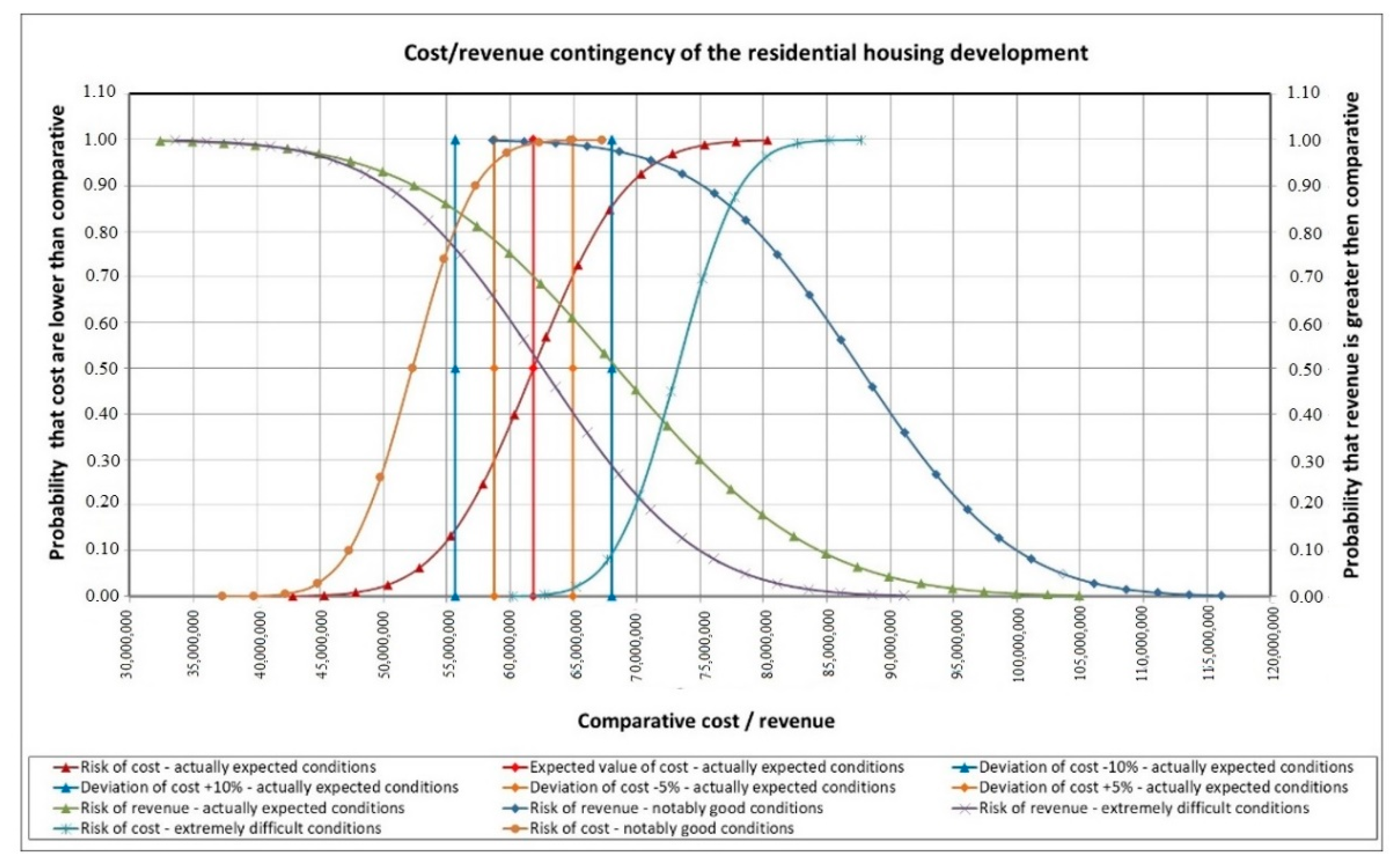
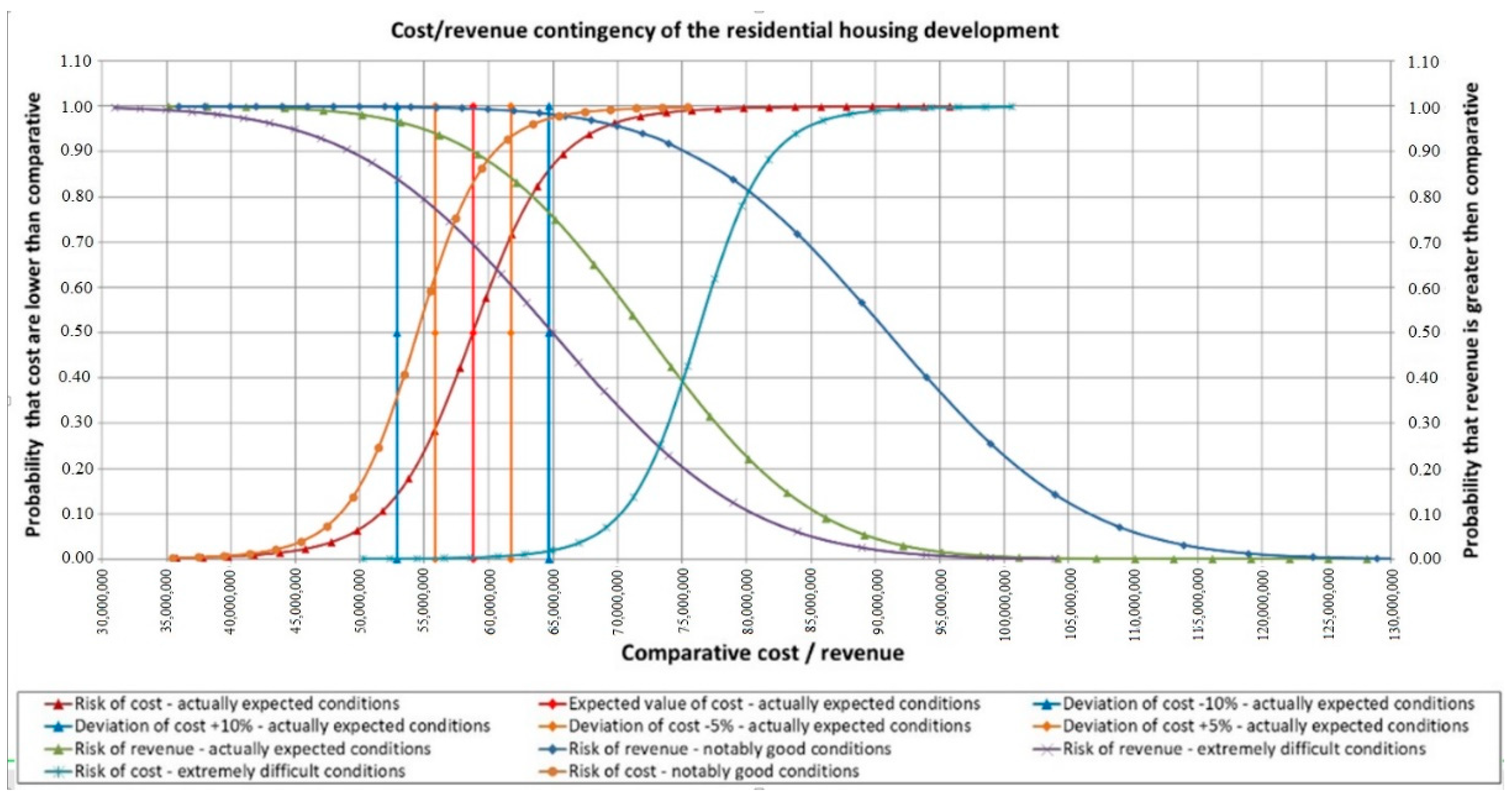
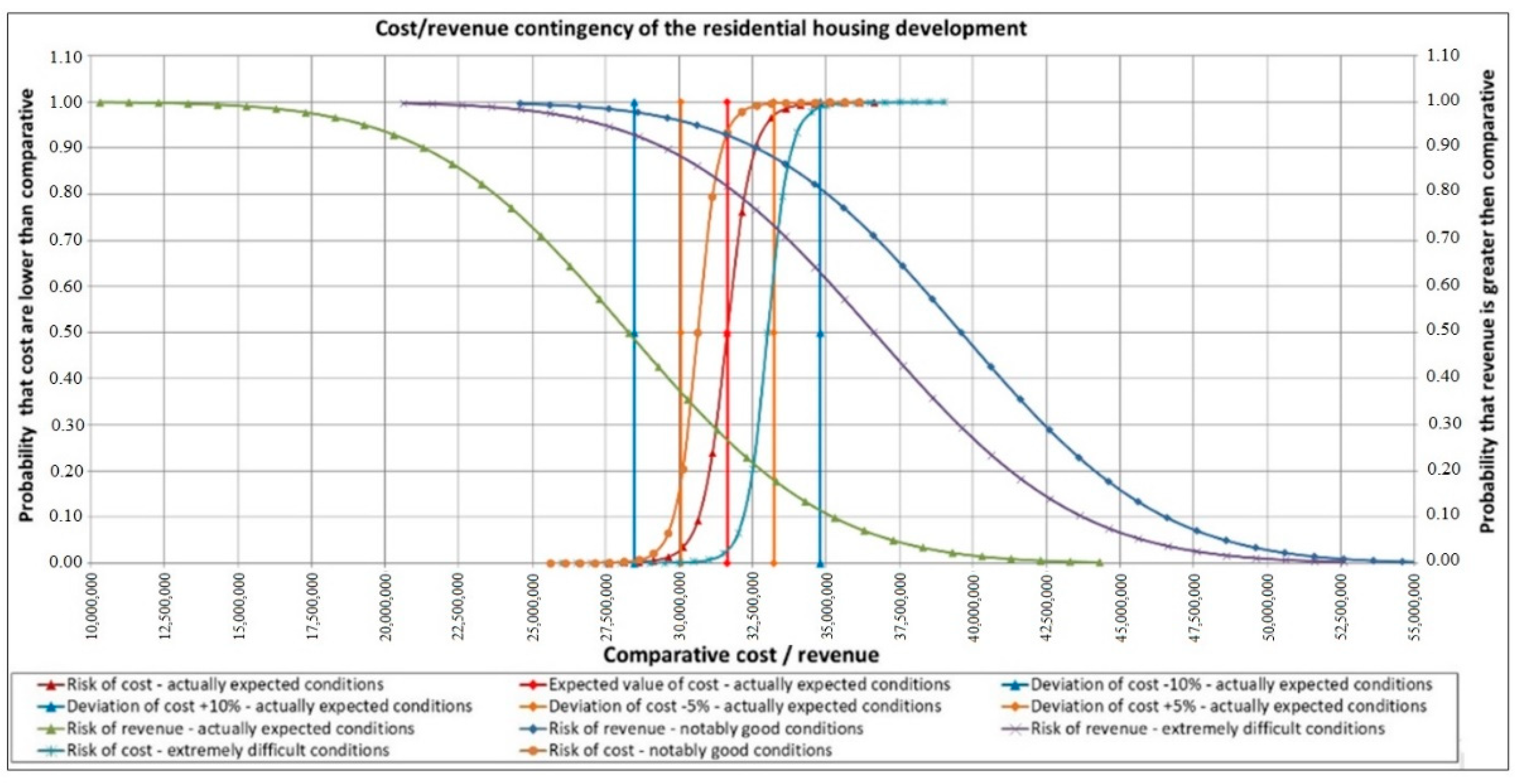
- Cost risk (contingency) of the project :—means probability that the real total cost should be less than k.
- Revenue risk (contingency) of the project :—means probability that the real overall revenue should be greater than d.
- Net present value of the residential housing development efficiency (NPE):
- Variance of efficiency:
- Standard deviation of efficiency:
- Expected gross profit E[Z]:
3. Results
3.1. Investment 2
3.2. Investment 3
4. Discussion
5. Conclusions
Author Contributions
Funding
Institutional Review Board Statement
Informed Consent Statement
Data Availability Statement
Conflicts of Interest
References
- Biznes, T. Słownik Pojęć Ekonomicznych; Wydawnictwo Naukowe PWN S.A.: Warszawa, Poland, 2007; ISBN 978-83-01-15279-6. [Google Scholar]
- Black, J. Słownik Ekonomii; Wydawnictwo Naukowe PWN: Warszawa, Poland, 2008; ISBN 978-83-01-15079-2. [Google Scholar]
- Pawłowski, J. Metodyka Oceny Efektywności Finansowej Przedsięwzięć Gospodarczych; Wydawnictwo Uniwersytetu Łódzkiego: Łódź, Poland, 2004; ISBN 83-7171-785-7. [Google Scholar]
- Ziarkowski, R. Opcje Rzeczowe Oraz ich Zastosowanie w Formułowaniu i Ocenie Projektów Inwestycyjnych; Wydawnictwo Akademii Ekonomicznej: Katowice, Poland, 2004; ISBN 8372463018 (20+5). [Google Scholar]
- Pyszka, A. Istota Efektywności. Definicje i Wymiary; Zeszyty Naukowe Uniwersytetu Ekonomicznego w Katowicach; Uniwersytet Ekonomiczny w Katowicach, Wydział Zarządzania, Katedra Zarządzania Zasobami Ludzkimi, Studia Ekonomiczne: Katowicach, Poland, 2015; ISSN 2083-8611. [Google Scholar]
- Pačaiová, H.; Andrejiová, M.; Balažiková, M.; Tomašková, M.; Gazda, T.; Chomová, K.; Hijj, J.; Salaj, L. Methodology for Complex Efficiency Evaluation of Machinery Safety Measures in a Production Organization. Appl. Sci. 2021, 11, 453. [Google Scholar] [CrossRef]
- Starczyk-Kołbyk, A.; Kruszka, L. The influence of construction works disturbances on the EVM analysis outcomes—Case study, Archives of Civil Engineering. Arch. Civ. Eng. 2020, 66, 161–177. [Google Scholar] [CrossRef]
- Starczyk-Kołbyk, A.; Kruszka, L. Use of the EVM method for analysis of extending the construction project duration as a result of realization disturbances—Case study. Arch. Civ. Eng. 2021, 67, 373–393. [Google Scholar] [CrossRef]
- Kasprowicz, T. Inżynieria Przedsięwzięć Budowlanych; Kasprowicz, T., Ed.; Inżynieria Przedsięwzięć Budowlanych, Rekomendowane Metody i Techniki, wyd.; PAN KIWiL, Sekcja IPB: Warszawa, Poland, 2015; pp. 10–20. [Google Scholar]
- Kasprowicz, T. Analiza Ryzyka Przedsięwzięć Budowlanych, Budownictwo i Inżynieria Środowiska, Zeszyt 58, nr 3/2011/III; Oficyna Wydawnicza Politechniki Rzeszowskiej: Rzeszów, Poland, 2011; pp. 233–240. [Google Scholar]
- Bizon-Górecka, J. O zarządzaniu projektami inwestycyjno-budowlanymi z uwzględnieniem czynników ryzyka. Przegląd Bud. 2008, 79, 42–46. [Google Scholar]
- Cao, J.; Song, W. Risk assessment of co-creating value with customers: A rough group analytic network process approach. Expert Syst. Appl. 2016, 55, 145–156. [Google Scholar] [CrossRef]
- Radło, M.J. Risk Management in Integrated Management Systems; Warsaw School of Economics: Warsaw, Poland, 2015. [Google Scholar]
- Kalkhoran, S.H.A.; Liravi, G.; Rezagholi, F. Risk Management in Construction Projects. Int. J. Eng. Trends Technol. 2014, 10, 133–138. [Google Scholar] [CrossRef]
- Ward, S.C.; Chapman, C.B. Risk-management perspective on the project lifecycle. Int. J. Proj. Manag. 1995, 13/3, 145–149. [Google Scholar] [CrossRef]
- Korytárová, J.; Hromádka, V. Risk Assessment of Large-Scale Infrastructure Projects—Assumptions and Context. Appl. Sci. 2021, 11, 109. [Google Scholar] [CrossRef]
- Gorlewski, B. Project Effectiveness Evaluation; Warsaw School of Economics: Warsaw, Poland, 2015. [Google Scholar]
- Pham, T.Q.D.; Le-Hong, T.; Tran, X.V. Efficient estimation and optimization of building costs using machine learning. Int. J. Constr. Manag. 2021. [Google Scholar] [CrossRef]
- JASPERS. Blue Book. Road Infrastructure. Joint Assistance to Support Projects in European Regions; Ministry of Infrastructure: Warsaw, Poland, 2008.
- De Wilde, P. Building Performance Analysis; John Wiley and Sons Ltd.: Hoboken, NJ, USA, 2018. [Google Scholar]
- Ding, L.; Zhou, Y.; Akinci, B. Building Information Modeling (BIM) application framework: The process of expanding from 3D to computable nD. Autom. Constr. 2014, 46, 82. [Google Scholar] [CrossRef]
- Halpin, D.W.; Woodhead, R.W. Construction Management, 2nd ed.; John Wiley & Sons Inc.: New York, NY, USA, 1998. [Google Scholar]
- Ritz, G. Total Construction Project Management; McGraw Hill Professional: New York, NY, USA, 1994. [Google Scholar]
- Benjamin, J.R.; Cornell, C.A. Probability, Statistics, and Decision for Civil Engineers; Manufactured in the United States by Courier Corporation: New York, NY, USA, 2014. [Google Scholar]
- Hajdu, M.; Bokor, O. Sensitivity analysis in PERT networks: Does activity duration distribution matter? Autom. Constr. 2016, 65, 1–8. [Google Scholar] [CrossRef]
- Skov, N.W. Finance & Management; The American Model Applied to Polish Private Enterprise; PRET: Warsaw, Poland, 1994. [Google Scholar]
- Frishman, F. On the Arithmetic Means and Variances of Products and Ratios of Random Variables; Army Research Office: Durham, UK, 1971; Available online: https://www.semanticscholar.org/paper/On-the-Arithmetic-Means-and-Variances-of-Products-Frishman/5116dc6b2987ee3eb26eab0a514c8a4a2e2b953c (accessed on 20 December 2021). [CrossRef]
- Parmenter, D. Key Performance Indicators: Developing, Implementing, and Using Winning KPIs; Copyright by David Parmenter; John Wiley & Sons, Inc.: Hoboken, NJ, USA, 2015. [Google Scholar]
- Braganca, L.; Kokkari, H.; Veljkovic, M.; Borg, R.P. Sustainable Construction. A Life Cycle Approach in Engineering; International Training School: Hal Far, Malta, 2010. [Google Scholar]
- Sicotte, H.; Delerue, H. Project planning, top management support and communication: A trident in search of an explanation. J. Eng. Technol. Manag. 2021, 60, 101626. [Google Scholar] [CrossRef]
- Uher, T.E.; Lawson, W. Sustainable development in construction. In Proceedings of the CIB World Building Congress, Gaevle, Sweden, 7–12 June 1998; pp. 1–8. [Google Scholar]


| Stages s | PLN | Ki PLN | ||||
|---|---|---|---|---|---|---|
| s1 | 100,000 | 3 | 0.6 | 98,242 | ||
| 12,300,000 | 3 | 0.6 | 12,083,779 | |||
| 3,500,000 | 3 | 0.6 | 3,438,474 | |||
| 6,400,000 | 3 | 0.6 | 6,287,495 | |||
| 3,400,000 | 3 | 0.6 | 3,340,232 | |||
| s2 | 200,000 | 4 | 1.5 | 1,885,732 | ||
| 200,000 | 4 | 1.5 | 188,573 | |||
| 200,000 | 4 | 1.5 | 188,573 | |||
| 600,000 | 4 | 1.5 | 565,720 | |||
| 600,000 | 4 | 1.5 | 565,720 | |||
| 200,000 | 4 | 1.5 | 188,573 | |||
| s3 | 200,000 | 4 | 3 | 177,799 | ||
| 10,500,000 | 4 | 3 | 9,334,462 | |||
| 3,500,000 | 4 | 3 | 3,111,487 | |||
| 16,500,000 | 4 | 3 | 14,668,440 | |||
| 3,500,000 | 4 | 3 | 3,111,487 | |||
| 3,950,000 | 4 | 3 | 3,511,536 | |||
| 1,000,000 | 4 | 3 | 888,996 | |||
| 500,000 | 4 | 3 | 444,498 | |||
| s4 | 100,000 | 4 | 3 | 88,900 | ||
| 200,000 | 4 | 6 | 158,063 | |||
| 150,000 | 4 | 5 | 123,289 | |||
| Sum | Total primary cost | 67,800,000 | Discounted total primary cost | 62,752,911 | ||
| Revenue | pi PLN | Di PLN | |||
|---|---|---|---|---|---|
| Tranches | b1 | 11,100,000 | 4 | 3 | 9,867,860 |
| b2 | 68,900,000 | 4 | 5 | 56,630,778 | |
| b3 | 6,200,000 | 4 | 5 | 5,095,948 | |
| b4 | 4,100,000 | 4 | 4 | 3,504,697 | |
| Sum | Overall revenue | 90,300,000 | Discounted overall revenue | 75,099,282 | |
| s | ||||||||
|---|---|---|---|---|---|---|---|---|
| s1 | 98,379 | 24,888 | 98,242 | 172,415 | 0.75 | 0.76 | ||
| 11,966,298 | 2,676,893 | 12,083,779 | 20,785,778 | 0.78 | 0.72 | |||
| 3,371,615 | 670,741 | 3,438,474 | 5,805,051 | 0.80 | 0.69 | |||
| 6,252,564 | 1,467,082 | 6,287,495 | 10,898,324 | 0.77 | 0.73 | |||
| 3,312,396 | 753,640 | 3,340,232 | 5,759,812 | 0.77 | 0.72 | |||
| Sum | 25,001,252 | |||||||
| s2 | 184,487 | 35,565 | 188,573 | 317,067 | 0.81 | 0.68 | ||
| 185,745 | 38,808 | 188,573 | 321,366 | 0.79 | 0.70 | |||
| 185,745 | 38,469 | 188,573 | 321,706 | 0.80 | 0.71 | |||
| 554,405 | 109,297 | 565,720 | 954,256 | 0.81 | 0.69 | |||
| 557,234 | 115,973 | 565,720 | 964,552 | 0.80 | 0.71 | |||
| 185,745 | 38,469 | 188,573 | 321,706 | 0.80 | 0.71 | |||
| Sum | 1,853,360 | |||||||
| s3 | 174,540 | 34,671 | 177,799 | 301,370 | 0.81 | 0.70 | ||
| 9,210,002 | 1,941,568 | 9,334,462 | 15,980,599 | 0.79 | 0.71 | |||
| 3,054,443 | 609,852 | 3,111,487 | 5,270,859 | 0.80 | 0.69 | |||
| 14,350,624 | 2,745,932 | 14,668,440 | 24,684,051 | 0.81 | 0.68 | |||
| 3,070,001 | 653,412 | 3,111,487 | 5,320,643 | 0.79 | 0.71 | |||
| 3,470,568 | 752,171 | 3,511,536 | 6,025,093 | 0.79 | 0.72 | |||
| 872,698 | 174,954 | 888,996 | 1,505,249 | 0.80 | 0.69 | |||
| 436,349 | 87,477 | 444,498 | 752,624 | 0.80 | 0.69 | |||
| Sum | 34,639,225 | |||||||
| s4 | 85,936 | 14,188 | 88,900 | 145,831 | 0.84 | 0.64 | ||
| 152,267 | 23,978 | 158,063 | 257,374 | 0.85 | 0.63 | |||
| 120,207 | 22,266 | 123,289 | 205,819 | 0.82 | 0.67 | |||
| 358,410 61,852,242 |
| Revenue | |||||||
|---|---|---|---|---|---|---|---|
| Tranches | b1 | 8,943,077 | 799,297 | 9,867,860 | 13,387,725 | 0.92 | 0.36 |
| b2 | 51,734,858 | 5,436,555 | 56,630,778 | 78,449,484 | 0.90 | 0.39 | |
| b3 | 4,611,152 | 302,699 | 5,095,948 | 6,980,419 | 0.94 | 0.37 | |
| b4 | 3,138,317 | 208,179 | 3,504,697 | 4,602,936 | 0.94 | 0.31 | |
| 68,427,404 68,427,404 |
| Primary Initial Data | Prediction for Risk Conditions | Real Conditions ex Post | |
|---|---|---|---|
| Notably good conditions of property sale | Complicated conditions of property sale | Complicated conditions of property sale | |
| Notably good conditions at labor and construction products market | Extremely difficult conditions at labor and construction products market | Extremely difficult conditions at labor and construction products market | |
| Specification | Primary value | Calculated value | Realized value |
| Expected conditions (0,xx) | |||
| Revenue | 90,300,000 | 68,534,790 | 66,990,000 |
| Cost | 67,800,000 | 61,743,054 | 60,939,000 |
| Efficiency | 1.33 | 1.11 | 1.10 |
| Gross profit | 22,500,000 | 6,791,736 | 6,051,000 |
| Notably good conditions (0,00) | |||
| Revenue | 87,853,537 | ||
| Cost | 52,293,772 | ||
| Efficiency | 1.68 | ||
| Gross profit | 35,559,765 | ||
| Extremely difficult conditions (1,00) | |||
| Revenue | 62,229,589 | ||
| Cost | 73,211,281 | ||
| Efficiency | 0.85 | ||
| Gross profit | −10,981,692 | ||
| Primary Initial Data | Prediction for Risk Conditions | Real Conditions ex Post | |
|---|---|---|---|
| Notably good conditions of property sale | Complicated conditions of property sale | Complicated conditions of property sale | |
| Notably good conditions at labor and construction products market | Extremely difficult conditions at labor and construction products market | Extremely difficult conditions at labor and construction products market | |
| Specification | Primary value | Calculated value | Realized value |
| Expected conditions (0,xx) | |||
| Revenue | 87,700,000 | 72,190,231 | 69,638,000 |
| Cost | 70,530,000 | 58,782,084 | 56,847,000 |
| Efficiency | 1.24 | 1.23 | 1.23 |
| Gross profit | 17,170,000 | 13,408,147 | 12,791,000 |
| Notably good conditions (0,00) | |||
| Revenue | 90,959,144 | ||
| Cost | 54,454,291 | ||
| Efficiency | 1.67 | ||
| Gross profit | 36,504,853 | ||
| Extremely difficult conditions (1,00) | |||
| Revenue | 64,970,817 | ||
| Cost | 76,236,008 | ||
| Efficiency | 0.85 | ||
| Gross profit | −11,265,190 | ||
| Primary Initial Data | Prediction for Risk Conditions | Real Conditions ex Post | |
|---|---|---|---|
| Notably good conditions of property sale | Complicated conditions of property sale | Complicated conditions of property sale | |
| Notably good conditions at labor and construction products market | Extremely difficult conditions at labor and construction products market | Extremely difficult conditions at labor and construction products market | |
| Specification | Primary value | Calculated value | Realized value |
| Expected conditions (0,xx) | |||
| Revenue | 38,190,000 | 36,631,885 | 40,585,000 |
| Cost | 32,500,000 | 31,641,704 | 34,591,000 |
| Efficiency | 1.18 | 1.16 | 1.17 |
| Gross profit | 5,690,000 | 4,990,181 | 5,994,000 |
| Notably good conditions (0,00) | |||
| Revenue | 39,609,233 | ||
| Cost | 30,632,977 | ||
| Efficiency | 1.29 | ||
| Gross profit | 8,976,255 | ||
| Extremely difficult conditions (1,00) | |||
| Revenue | 28,292,309 | ||
| Cost | 33,016,968 | ||
| Efficiency | 0.86 | ||
| Gross profit | −4,724,659 | ||
Publisher’s Note: MDPI stays neutral with regard to jurisdictional claims in published maps and institutional affiliations. |
© 2021 by the authors. Licensee MDPI, Basel, Switzerland. This article is an open access article distributed under the terms and conditions of the Creative Commons Attribution (CC BY) license (https://creativecommons.org/licenses/by/4.0/).
Share and Cite
Kasprowicz, T.; Starczyk-Kołbyk, A.; Wójcik, R. Randomized Estimation of the Net Present Value of a Residential Housing Development. Appl. Sci. 2022, 12, 124. https://doi.org/10.3390/app12010124
Kasprowicz T, Starczyk-Kołbyk A, Wójcik R. Randomized Estimation of the Net Present Value of a Residential Housing Development. Applied Sciences. 2022; 12(1):124. https://doi.org/10.3390/app12010124
Chicago/Turabian StyleKasprowicz, Tadeusz, Anna Starczyk-Kołbyk, and Robert Wójcik. 2022. "Randomized Estimation of the Net Present Value of a Residential Housing Development" Applied Sciences 12, no. 1: 124. https://doi.org/10.3390/app12010124