
No-Reference Image Quality Assessment with Convolutional Neural Networks and Decision Fusion


Ronin Institute, Montclair, NJ 07043, USA
Appl. Sci. 2022, 12(1), 101; https://doi.org/10.3390/app12010101
Submission received: 29 November 2021
/
Revised: 20 December 2021
/
Accepted: 21 December 2021
/
Published: 23 December 2021
(This article belongs to the Special Issue Advances in Intelligent Control and Image Processing)
Abstract
:No-reference image quality assessment (NR-IQA) has always been a difficult research problem because digital images may suffer very diverse types of distortions and their contents are extremely various. Moreover, IQA is also a very hot topic in the research community since the number and role of digital images in everyday life is continuously growing. Recently, a huge amount of effort has been devoted to exploiting convolutional neural networks and other deep learning techniques for no-reference image quality assessment. Since deep learning relies on a massive amount of labeled data, utilizing pretrained networks has become very popular in the literature. In this study, we introduce a novel, deep learning-based NR-IQA architecture that relies on the decision fusion of multiple image quality scores coming from different types of convolutional neural networks. The main idea behind this scheme is that a diverse set of different types of networks is able to better characterize authentic image distortions than a single network. The experimental results show that our method can effectively estimate perceptual image quality on four large IQA benchmark databases containing either authentic or artificial distortions. These results are also confirmed in significance and cross database tests.
1. Introduction
The aim of image quality assessment (IQA) is predicting digital images’ perceived quality that is consistent with the human visual system’s (HVS) perception [1]. The most obvious way to evaluate the quality of digital images is a subjective user study where quality scores are obtained from human observers in a laboratory environment [2] or a crowdsourcing experiment [3]. However, such experiments are expensive, laborious, and time consuming. Thus, they cannot be applied in a real-time system. On the other hand, they result in publicly available benchmark IQA databases, such as KonIQ-10k [4] or SPAQ [5], which consist of images with their quality scores. In most cases, quality scores are given as mean opinion scores (MOS), which are arithmetic averages of all quality opinions given by individual observers. In contrast, the aim of objective IQA is constructing computational, mathematical models that can estimate digital images’ human perceptual quality.
Traditionally, objective IQA is divided into three branches in the literature based on the availability of the distortion-free reference images. The first branch is no-reference image quality assessment (NR-IQA) where no information is available about the reference images. Contrarily, full-reference image quality assessment (FR-IQA) methods have full access to the reference images, while reduced-reference image quality assessment (RR-IQA) models have only partial information about the reference images.
Recently, deep learning has dominated the field of image processing and computer vision. The field of objective IQA has not been an exception to this trend. The goal of this study is to introduce a novel deep learning-based NR-IQA method for authentic distortions that relies on decision fusion of multiple quality scores coming from different types of convolutional neural network architectures. The proposed decision fusion-based model allows us to better characterize authentic image distortions due to the diverse set of different types of networks.
The rest of this section is organized as follows. First, related and previous work is reviewed in Section 1.1. Second, the main contributions of this study are enumerated in Section 1.2 in light of previous work. Third, the structure of the paper is defined in Section 1.3.
1.1. Related Work
In recent decades, a lot of NR-IQA methods have been published in the literature. NR-IQA models can be divided into two categories, such as distortion-specific and general methods. Specifically, distortion-specific methods assume a certain distortion type (e.g., blur [6] or JPEG compression noise [7]) present in the image, while general algorithms do not make any assumptions about the noise or distortion type present in the image. Early NR-IQA methods mainly fell into the distortion-specific category. On the other hand, general NR-IQA algorithms can be divided into three groups, i.e., natural scene statistics (NSS)-based, HVS-based, and learning-based ones.
1.1.1. NSS-Based Methods
The main assumption behind NSS-based methods is that natural images of high quality have certain statistical features which lose strength in the presence of image noise and degradation. A typical NSS-based algorithm has three distinct stages, i.e., feature extraction, NSS modeling and regression [8]. A representative example of NSS-based methods was proposed by Moorthy and Bovik [9]. Namely, the statistical properties of wavelet coefficients were utilized as quality-aware features using a Gaussian scale mixture model in the authors’ work. Another well-known example is the blind image quality index (BIQI) [10] which works with wavelet transform to decompose an input image into three scales and orientations. Next, generalized Gaussian distributions (GGD) were fitted onto the wavelet coefficients and the mean, the variance and the shape parameters of the GGDs were considered as quality-aware features. These were mapped onto perceptual quality scores with a trained support vector regressor (SVR). NSS-based methods have been proposed in other transform domains, i.e., curvelet [11], contourlet [12], quaternion wavelet transform [13] and discrete cosine transform [14] and in the spatial domain [15], as well.
1.1.2. HVS-Based Methods
In contrast to NSS-based methods, HVS-based approaches try to utilize one or more computational aspects of the HVS to devise an NR-IQA algorithm. For example, Zhai et al. [16] employed the free-energy principle [17] and considered the visual quality assessment of an image as an active inference process. Similarly, Gu et al. [18] applied the free-energy principle but it was improved by structural and gradient information. Li et al. [19] utilized the observation of previous studies [20,21] that the HVS is conformed to extract structural information from images. Thus, the authors introduced a special variant of local binary pattern [22] operators on the luminance map to describe the structural information. In [23], the authors took the same assumption, but first- and second-order image structures were extracted to characterize the structural information of an image. Namely, Prewitt filters [24] were applied for first-order image structure extraction, while local contrast normalization [25] was used for second-order image structure extraction. On the other hand, Saha and Wu [26] built on redundancy and scale invariance properties of natural images [27].
1.1.3. Learning-Based Methods
Learning-based methods heavily rely on data-driven techniques, such as deep learning. First, Kang et al. [28] applied convolutional neural network (CNN) for NR-IQA. Namely, the authors trained a CNN of five layers from scratch on locally normalized image patches. The overall quality estimation was obtained by averaging the image patches’ quality scores. Similarly, Bosse et al. [29] trained a patch-based CNN, but a patch weighting scheme was also developed to reflect the importance of individual patches in quality estimation. Jia and Zhang [30] assigned weights to image patches using image saliency. In [31], the predicted quality scores of image patches were directly weighted by local image saliency. In contrast, Chetouani and Li [32] proposed a specific scanpath predictor, which mimics the movements of the human eye [33], for image patch selection. Fan et al. [34] developed multi-expert CNNs for evaluating the perceptual quality of artificially distorted images. Namely, the authors trained a CNN for each possible distortion type (JPEG, JPEG2000, Gaussian, etc.) of an IQA benchmark database and a distortion identification network. The outputs of the previously mentioned networks were combined to obtain an input image’s perceptual quality. Another line of works deals with deep feature extraction for NR-IQA [35,36,37,38,39,40]. Namely, the first layers of a CNN usually capture elemental image features, such as blobs, edges, boundaries and color patterns, which are quality-aware features [41]. First, Bianco et al. [35] applied deep features extracted from pretrained CNNs for perceptual image quality estimation. Namely, random patches were sampled from an input image and deep features were derived from each patch. Subsequently, the extracted deep feature vectors were pooled together and mapped onto quality scores with a trained SVR. In [36], the inception modules [42] of a CNN and global average pooling layers were used to compile deep features which were mapped onto perceptual quality with an SVR. In contrast, Chetouani et al. [39] combined viewing distance information with deep features to obtain a better performance. Su and Korhonen [43] introduced weighted spatial pooling to aggregate arbitrarily sized spatial feature maps into a feature vector which is mapped onto quality scores with the help of a fully connected layer. In [40,44], a multi-scale representation was constructed from deep features to get an effective image representation for NR-IQA. In contrast, Korhonen et al. [45] utilized a recurrent neural network for spatial pooling of deep features. Ying et al. [46] applied the pooling of regions’ of interest features and the training across multiple IQA benchmark databases.
1.2. Contributions
The main contributions of this study are as follows: (i) decision fusion of deep convolutional architectures for NR-IQA. (ii) The usage of a diverse set of pretrained convolutional architectures to better characterize natural images’ authentic distortions. (iii) Extensive evaluation of different deep architectures on large IQA benchmark databases.
1.3. Structure
The remainder of this study is organized as follows. Section 2 can be divided into two main parts. First, the tools applied in our experiments are introduced. Next, the proposed method is presented. Section 3 gives the experimental results and performance analysis of the proposed approach. Moreover, it presents a comparison to other state-of-the-art methods. Finally, a conclusion is drawn in Section 4 with possible directions of future research.
2. Materials and Methods
In this section, the tools applied in our experiments and the proposed method are described. Specifically, Section 2.1 reports on the applied publicly available databases, evaluation protocol and implementation details. In Section 2.2, the proposed method is introduced in detail.
2.1. Materials
2.1.1. Databases
As already mentioned, a number of benchmark IQA databases have been made publicly available in the recent decades [8,47,48,49]. In this study, we deal with the quality assessment of natural images containing authentic distortions. To evaluate and compare our proposed method to the state of the art, three large databases—LIVE In the Wild (CLIVE) [50], KonIQ-10k [4] and SPAQ [5]—with authentic distortions have been chosen. Moreover, one database—TID2013 [51]—with artificial distortions was also utilized in our experiments. In the following, a brief overview is given about the previously mentioned IQA benchmark databases.
Ghadiyaram et al. [50] collected 1162 images with unique scenes captured by a variety of mobile device cameras. Subsequently, these images were evaluated in a crowdsourcing experiment to obtain MOS values (ranging from 0 to 100). Similarly to CLIVE, the images of KonIQ-10k [4] were evaluated in a crowdsourcing experiment. An important difference between CLIVE [50] and KonIQ-10k [4] is that the images of KonIQ-10k were collected from the YFCC-100m [52] multimedia database using a two-stage filtering process. First, those images were discarded which did not have a creative commons license. Second, such a filtering process was applied that enforces the relative uniform distribution of eight image attributes, i.e., bitrate, resolution, JPEG quality, brightness, colorfulness, contrast, sharpness and deep feature. The MOS range in KonIQ-10k [4] spans from 1 to 5. Fang et al. [5] collected 11,125 high-resolution digital images captured by 66 smartphones. Subsequently, the collected images were evaluated in a laboratory environment involving 600 subjects. Moreover, the MOS values of each image have been determined based on at least 15 quality scores. In contrast to the previously mentioned databases, TID2013 [51] contains images with artificial distortions. Specifically, it contains a set of 25 pristine reference images whose perceptual quality are considered perfect. From these reference images, 3000 distorted images are derived using 24 different types of distortions at five distortion levels.
2.1.2. Evaluation Protocol and Implementation Details
The evaluation of NR-IQA algorithms is based on the correlation strength measured between predicted and ground-truth scores. To characterize the correlation strength, the Pearson linear correlation coefficient (PLCC), Spearman rank order correlation coefficient (SROCC) and Kendall rank order correlation coefficient (KROCC) are widely applied in the literature [8]. Moreover, before the calculation of PLCC, a non-linear mapping is carried out between the predicted and ground-truth scores using a logistic function with 5 parameters, as recommended by Sheikh et al. [53]. Formally, this non-linear mapping can be given as
where ’s are the fitting parameters. Moreover, and Q denote the predicted and mapped quality scores, respectively. Between vectors and of the same length N, PLCC is defined as
where , denote the ith element of , , respectively. Moreover, and . Between these vectors, SROCC is defined as
where stands for the difference between the two ranks of each and . Moreover, the following formula is used to determine KROCC
where C is the number of concordant pairs between and , while D is the number of discordant pairs.
As is common in the literature [8], we report on median PLCC, SROCC and KROCC values measured over 100 random train-validation-test splits. Since the median is more robust to outliers, it is preferred in the literature to arithmetic mean. More precisely, an IQA benchmark database containing authentic distortions (CLIVE [50], KonIQ-10k [4] and SPAQ [5]) was randomly divided into a training set with approximately 70% of images, a validation set with 10% of images, and a test set with the remaining 20%. Since TID2013 [51] consists of images with artificial distortions, it was divided with respect to the reference images to avoid any semantic content overlap between the train, validation and test sets.
The proposed method was implemented in Python 3.6.1 programming language using the Keras deep learning library [54] and the Keras utilities (Kuti) library. Moreover, the proposed method was trained on two NVidia Titan Xp GPUs.
2.2. Methods
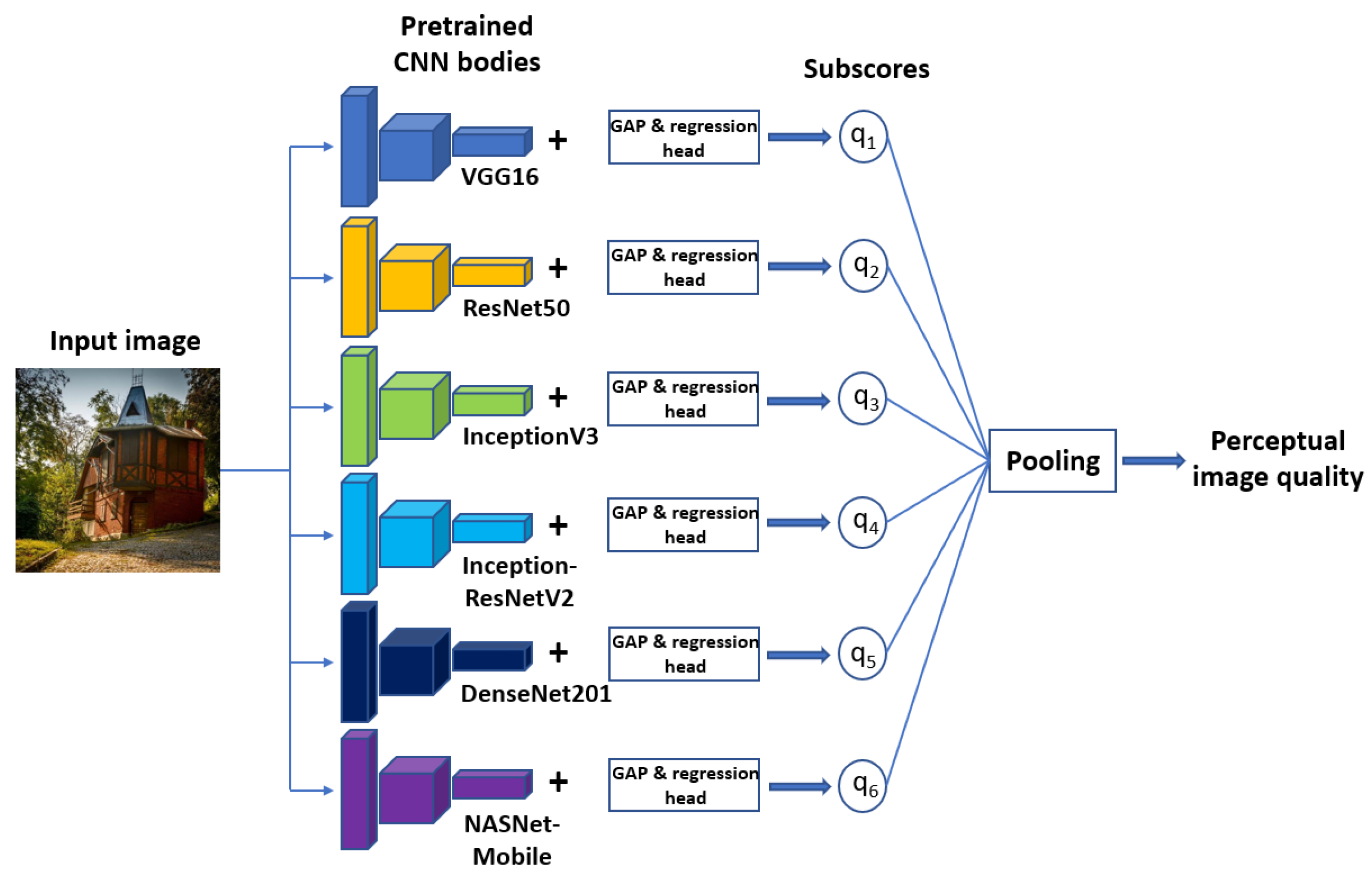
The high-level overview of the proposed end-to-end method is depicted in Figure 4. An input image to be evaluated is passed through six in-parallel state-of-the-art CNN bodies pretrained on ImageNet [55] database for image classification, such as VGG16 [56], ResNet50 [57], InceptionV3 [58], InceptionResNetV2 [59], DenseNet201 [60] and NASNetMobile [61], succeeded by global average pooling layers and regression heads. The main characteristics of the applied CNNs are summarized in Table 2. It is important to note that the fully connected output layers of these models were not utilized in this work, allowing us to attach new layers to them and train them for NR-IQA. Moreover, the pretrained CNN body term is reserved for a deep model without the fully connected output layers in our terminology.
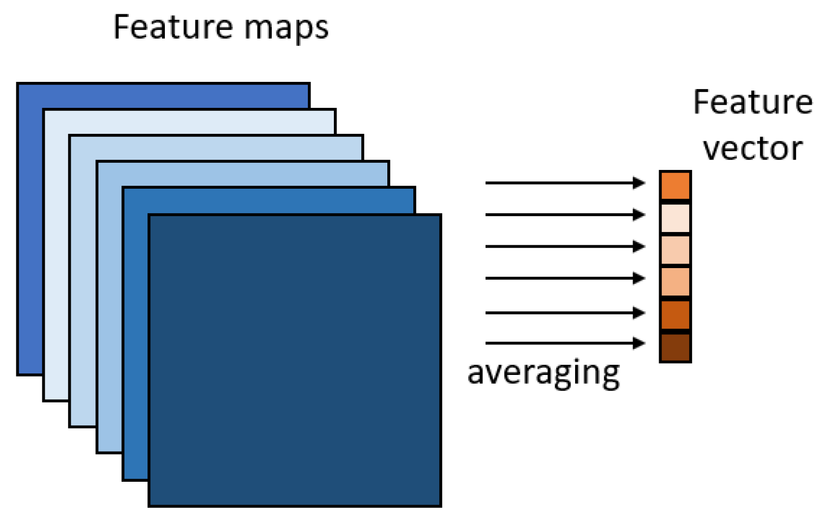
The main idea behind global average pooling (illustrated in Figure 5) is to enforce correspondences between feature maps and the number of predicted semantic categories by taking the average of each feature map and compiling a feature vector. Thus, arbitrary sized images can be put to the input of a CNN. Other advantages are that overfitting can be avoided with this layer and robustness can be increased against spatial translations of the input [63].
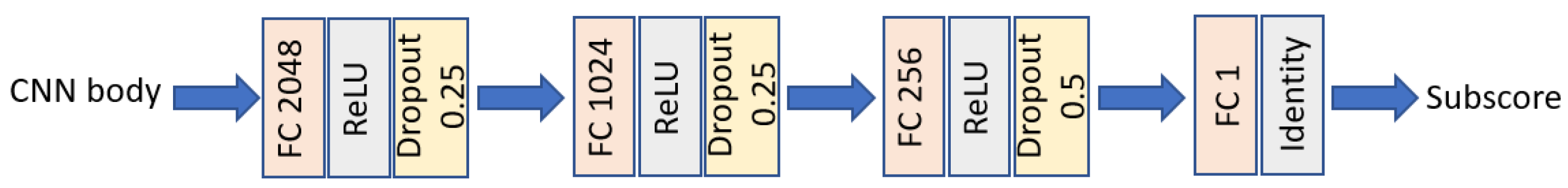
The outputs of the global average pooling layers are connected to six regression heads containing four separately fully connected layers. The inner structure of the regression heads is depicted in Figure 6. Specifically, the first three layers consists of 2048, 1024 and 256 nodes, respectively. To avoid overfitting, these layers possess dropout rates [64] of 0.25, 0.25 and 0.5, respectively. To ensure better gradient propagation, rectified linear units (ReLU) were applied as activation functions in the first three layers [62]. Since the last layer predicts the quality, it contains only one neuron and applies a simple linear activation function. Let denote the training dataset, where is an RGB image of arbitrary size and q is the ground-truth quality score belonging to . Moreover, we denote by the quality score predicted by one regression head. Since image quality prediction is formulated as a regression task here, mean squared error (MSE) loss is applied, which—as the name suggests—takes the mean of squared differences between the ground-truth and predicted values. Formally, this can be written as: .
The six branches of the proposed fused architecture are trained using the same training and validation datasets but independently from each other. Specifically, a pretrained CNN body plus regression head structure was trained using the Adam [65] optimizer with the default parameters of the Keras [54] deep learning library and a batch size of 16. First, a model is trained through 40 epochs with a learning rate of . During training, the PLCC computed between the predicted and ground-truth quality scores on the validation set is monitored and after 40 epochs the best performing option is restored. Second, this restored model is trained through 20 epochs with a learning rate of . Similarly to the previous step, PLCC on the validation set is constantly monitored during the training process, and after 20 epochs, the best performing one is reloaded.
The quality predictions of the six branches are fused together to obtain an overall quality score for the input image. Specifically, average and median pooling were applied in this work. A parameter study was conducted to ascertain which is the better option (presented in Section 3.1).
3. Experimental Results and Analysis
In this section, detailed experimental results and analysis are presented. More specifically, Section 3.1 introduces a parameter study regarding the proposed method so that the justification of the proposed method’s design choices is possible. Next, a comparison to the state of the art is shown on the CLIVE [50] and KonIQ-10k [4] databases in Section 3.2.
3.1. Parameter Study
First, we examine the performance of the individual models which consist of a pretrained CNN body, global average pooling layer and a regression head. Second, we compare the effects of two different fusion of quality subscores, i.e., average and median pooling. The evaluation protocol is exactly the same as described in Section 2.1. The results obtained on KonIQ-10k [4] are summarized in Table 3. From these results, it can be concluded that using an optional pretrained CNN body results in a rather strong correlation between the predicted and ground-truth quality scores. On the other hand, the performance of VGG16 [56] and ResNet50 [57] lags behind those of the other pretrained networks. Further, regarding the decision fusion of different network types, both average and median pooling are able to increase the prediction performance substantially. Since median pooling outperforms average pooling, as one can see in Table 3, this was used in our NR-IQA method for a comparison to other state-of-the-art algorithms.
3.2. Comparison to the State of the Art
To compare the proposed method to the state of the art, several NR-IQA methods have been collected, such as BLIINDER [66], DeepRN [67], BLIINDS-II [14], BMPRI [68], BRISQUE [15], CurveletQA [11], DIIVINE [9], ENIQA [69], GRAD-LOG-CP [70], MultiGAP- NRIQA [36], MSDF-IQA [40], NBIQA [71], PIQE [72], OG-IQA [73], SSEQ [74] and UNIQUE [75], whose original source codes are publicly available online. Excluding PIQE [72], which is an opinion-unaware method without a training step, these methods were evaluated using the same principle as the proposed method’s on the applied IQA benchmark databases (CLIVE [50], KonIQ-10k [4], SPAQ [5] and TID2013 [51]). As already mentioned, the median PLCC, SROCC and KROCC values are reported, which were measured over 100 random train–validation–test splits. Specifically, approximately 80% of images were in the training set, while the remaining 20% were in the test set, if a validation set is not required for an NR-IQA method. If a validation set is needed, then 70% of the images were in the training set, 10% in the validation set and 20% in the test set. Since TID2013 [51] contains images with artificial distortions, it was divided with respect to the reference images. Moreover, the performance results of several state-of-the-art deep learning-based methods, such as CONTRIQUE [76], DB-CNN [77], DeepFL-IQA [78], KonCept512 [79], MLSP [78,80], PaQ-2-PiQ [46], PQR [81] and WSP [43], were copied from the authors’ corresponding papers and added to our comparison. It is important to note that our proposed method was trained on down-sampled versions of KonIQ-10k [4] ( resolution instead of ) and SPAQ [5] ( resolution instead of ∼) due to graphics processing unit (GPU) memory limitations and to accelerate the training process. Further, our proposed method is codenamed as DF-CNN-IQA throughout the comparative tables published in this paper.
The experimental results obtained on CLIVE [50] and KonIQ-10k [4] are summarized in Table 4. From these results, it can be observed that the proposed method outperforms all the other considered methods on KonIQ-10k [4] by a large margin. Specifically, it outperforms the second- and third-best methods by approximately 0.01 in terms of PLCC and SROCC. On the smaller CLIVE, the proposed method gives the second-best results among the methods which were tested by us. According to our experiments, the UNIQUE [75] method was able to exceed DF-CNN-IQA.
The experimental results obtained on SPAQ [5] and TID2013 [51] are summarized in Table 5. From these results, it can be observed that DF-CNN-IQA excels the performance of all the other considered NR-IQA algorithms on SPAQ [5], while it performs weaker than the best state-of-the-art method on TID2013 [51], which in contrast to SPAQ [5] contains artificial distortions.
The direct and weighted averages obtained on these IQA databases are summarized in Table 6. It can be seen that the direct average PLCC, SROCC and KROCC values of the proposed method are larger than those of the majority of the considered state-of-the-art methods. If we take a look at the weighted average by the number of images found in the applied IQA benchmark databases, the difference between the proposed method and the other methods is even more significant. Specifically, DF-CNN-IQA can outperform all the other algorithms in this regard. Moreover, it can be concluded that the proposed method tends to give a better performance on larger IQA benchmark databases with authentic distortions.
To ascertain whether the achieved results are significant or not, one-sided t-tests [83] were carried out between the 100 SROCC values produced by our and the other state-of-the-art methods tested by us. Namely, the null hypothesis was that the mean SROCCs of two sets containing 100–100 correlation values are equal with a confidence of 95%. The results of the one-sided t-tests are summarized in Table 7. In this table, symbol 1 stands for that the proposed method is statistically better (worse) at a confidence interval of than the other examined NR-IQA method. From these results, it can be concluded that the proposed method is able to significantly outperform the state of the art on large databases with authentic distortions (KonIQ-10k [4] and SPAQ [5]), while it is outperformed by two methods on artificial distortions (TID2013 [51]).
To further demonstrate the effectiveness of the proposed method, a cross-database test was also carried out, where the examined algorithms were trained on the large KonIQ-10k [4] and tested on the smaller CLIVE [50]. The results of this cross-database test are summarized in Table 8. From the presented results, it can be seen that the proposed method is able to outperform all the other considered algorithms by a large margin. This means that the proposed method possesses a rather strong generalization capability.
4. Conclusions
In this paper, we proposed a novel deep learning-based approach for NR-IQA. Specifically, a decision fusion of different deep convolutional architectures, such as VGG16 [56], ResNet50 [57], InceptionV3 [42], InceptionResNetV2 [59], DenseNet201 [60] and NASNetMobile [61], were carried out to for perceptual image quality estimation. The main motivation behind this layout was the following. The first layers of a CNN frequently capture basic image structures, i.e., edges, blobs or color patterns, which are quality-aware features. Using a diverse set of pretrained CNNs allowed us to better characterize natural images’ authentic distortions. This motivation was confirmed in a parameter study where it was demonstrated that a decision fusion of CNNs is able to considerably improve the performance of estimation. In a series of comparative experiments, it has been shown that the proposed method is able to reach or outperform the state of the art on two IQA benchmark databases with authentic distortions. The obtained results were confirmed in significance and cross-database tests. Future work will focus on a feature-level fusion and joint training of CNNs to reduce the training time and to achieve simpler architectures. Another direction of research is to generalize the achieved results for specific applications, such as the quality assessment of computer tomography (CT) or magnetic resonance imaging (MRI) images. The source code of the proposed is available at: https://github.com/Skythianos/DF-CNN-IQA, accessed on 28 November 2021.
Funding
This research received no external funding.
Institutional Review Board Statement
Not applicable.
Informed Consent Statement
Not applicable.
Data Availability Statement
The datasets used were obtained from publically open source datasets from: 1. CLIVE: https://live.ece.utexas.edu/research/ChallengeDB/index.html (accessed on 28 November 2021), 2. KonIQ-10k: http://database.mmsp-kn.de/koniq-10k-database.html (accessed on 28 November 2021), 3. SPAQ: https://github.com/h4nwei/SPAQ (accessed on 28 November 2021), 4. TID2013: http://www.ponomarenko.info/tid2013.htm (accessed on 28 November 2021).
Acknowledgments
We thank the anonymous reviewers for their careful reading of our manuscript and their many insightful comments and suggestions.
Conflicts of Interest
The author declares no conflict of interest.
Abbreviations
The following abbreviations are used in this manuscript:
| CNN | convolutional neural network |
| CT | computer tomography |
| FR-IQA | full-reference image quality assessment |
| GGD | generalized Gaussian distribution |
| GPU | graphics processing unit |
| HVS | human visual system |
| IQA | image quality assessment |
| JPEG | joint photographic experts group |
| KROCC | Kendall rank order correlation coefficient |
| LIVE | Laboratory of Image and Video Engineering |
| MOS | mean opinion score |
| MRI | magnetic resonance imaging |
| MSE | mean squared error |
| NR-IQA | no-reference image quality assessment |
| NSS | natural scene statistics |
| PLCC | Pearson linear correlation coefficient |
| ReLU | rectified linear unit |
| RR-IQA | reduced-reference image quality assessment |
| SPAQ | smartphone photography attribute and quality |
| SROCC | Spearman rank order correlation coefficient |
| SVR | support vector regressor |
| TID | Tampere image database |
| YFCC-100m | Yahoo Flickr creative commons 100 million dataset |
References
- Keelan, B. Handbook of Image Quality: Characterization and Prediction; CRC Press: Boca Raton, FL, USA, 2002. [Google Scholar]
- Chubarau, A.; Akhavan, T.; Yoo, H.; Mantiuk, R.K.; Clark, J. Perceptual image quality assessment for various viewing conditions and display systems. Electron. Imaging 2020, 2020, 67-1–67-9. [Google Scholar] [CrossRef]
- Saupe, D.; Hahn, F.; Hosu, V.; Zingman, I.; Rana, M.; Li, S. Crowd workers proven useful: A comparative study of subjective video quality assessment. In Proceedings of the QoMEX 2016: 8th International Conference on Quality of Multimedia Experience, Lisbon, Portugal, 6–8 June 2016. [Google Scholar]
- Lin, H.; Hosu, V.; Saupe, D. KonIQ-10K: Towards an ecologically valid and large-scale IQA database. arXiv 2018, arXiv:1803.08489. [Google Scholar]
- Fang, Y.; Zhu, H.; Zeng, Y.; Ma, K.; Wang, Z. Perceptual quality assessment of smartphone photography. In Proceedings of the IEEE/CVF Conference on Computer Vision and Pattern Recognition, Seattle, WA, USA, 14–19 June 2020; pp. 3677–3686. [Google Scholar]
- Serir, A.; Beghdadi, A.; Kerouh, F. No-reference blur image quality measure based on multiplicative multiresolution decomposition. J. Vis. Commun. Image Represent. 2013, 24, 911–925. [Google Scholar] [CrossRef]
- Babu, R.V.; Suresh, S.; Perkis, A. No-reference JPEG-image quality assessment using GAP-RBF. Signal Process. 2007, 87, 1493–1503. [Google Scholar] [CrossRef]
- Xu, L.; Lin, W.; Kuo, C.C.J. Visual Quality Assessment by Machine Learning; Springer: Berlin/Heidelberg, Germany, 2015. [Google Scholar]
- Moorthy, A.K.; Bovik, A.C. Blind image quality assessment: From natural scene statistics to perceptual quality. IEEE Trans. Image Process. 2011, 20, 3350–3364. [Google Scholar] [CrossRef] [PubMed]
- Moorthy, A.K.; Bovik, A.C. A two-step framework for constructing blind image quality indices. IEEE Signal Process. Lett. 2010, 17, 513–516. [Google Scholar] [CrossRef]
- Liu, L.; Dong, H.; Huang, H.; Bovik, A.C. No-reference image quality assessment in curvelet domain. Signal Process. Image Commun. 2014, 29, 494–505. [Google Scholar] [CrossRef]
- Lu, W.; Zeng, K.; Tao, D.; Yuan, Y.; Gao, X. No-reference image quality assessment in contourlet domain. Neurocomputing 2010, 73, 784–794. [Google Scholar] [CrossRef]
- Wang, H.; Li, C.; Guan, T.; Zhao, S. No-reference stereoscopic image quality assessment using quaternion wavelet transform and heterogeneous ensemble learning. Displays 2021, 69, 102058. [Google Scholar] [CrossRef]
- Saad, M.A.; Bovik, A.C.; Charrier, C. Blind image quality assessment: A natural scene statistics approach in the DCT domain. IEEE Trans. Image Process. 2012, 21, 3339–3352. [Google Scholar] [CrossRef] [PubMed]
- Mittal, A.; Moorthy, A.K.; Bovik, A.C. No-reference image quality assessment in the spatial domain. IEEE Trans. Image Process. 2012, 21, 4695–4708. [Google Scholar] [CrossRef]
- Zhai, G.; Wu, X.; Yang, X.; Lin, W.; Zhang, W. A psychovisual quality metric in free-energy principle. IEEE Trans. Image Process. 2011, 21, 41–52. [Google Scholar] [CrossRef] [PubMed]
- Friston, K.; Kilner, J.; Harrison, L. A free energy principle for the brain. J. Physiol. 2006, 100, 70–87. [Google Scholar] [CrossRef] [Green Version]
- Gu, K.; Zhai, G.; Yang, X.; Zhang, W. Using free energy principle for blind image quality assessment. IEEE Trans. Multimed. 2014, 17, 50–63. [Google Scholar] [CrossRef]
- Li, Q.; Lin, W.; Xu, J.; Fang, Y. Blind image quality assessment using statistical structural and luminance features. IEEE Trans. Multimed. 2016, 18, 2457–2469. [Google Scholar] [CrossRef]
- Nothdurft, H. Sensitivity for structure gradient in texture discrimination tasks. Vis. Res. 1985, 25, 1957–1968. [Google Scholar] [CrossRef]
- Watson, A.B.; Solomon, J.A. Model of visual contrast gain control and pattern masking. JOSA A 1997, 14, 2379–2391. [Google Scholar] [CrossRef] [Green Version]
- Ojala, T.; Pietikäinen, M.; Harwood, D. A comparative study of texture measures with classification based on featured distributions. Pattern Recognit. 1996, 29, 51–59. [Google Scholar] [CrossRef]
- Li, Q.; Lin, W.; Fang, Y. BSD: Blind image quality assessment based on structural degradation. Neurocomputing 2017, 236, 93–103. [Google Scholar] [CrossRef]
- Prewitt, J.M. Object enhancement and extraction. Pict. Process. Psychopictorics 1970, 10, 15–19. [Google Scholar]
- Lyu, S.; Simoncelli, E.P. Nonlinear image representation using divisive normalization. In Proceedings of the 2008 IEEE Conference on Computer Vision and Pattern Recognition, Anchorage, AK, USA, 23–28 June 2008; pp. 1–8. [Google Scholar]
- Saha, A.; Wu, Q.M.J. Utilizing image scales towards totally training free blind image quality assessment. IEEE Trans. Image Process. 2015, 24, 1879–1892. [Google Scholar] [CrossRef] [PubMed]
- Ruderman, D.L.; Bialek, W. Statistics of natural images: Scaling in the woods. Phys. Rev. Lett. 1994, 73, 814. [Google Scholar] [CrossRef] [Green Version]
- Kang, L.; Ye, P.; Li, Y.; Doermann, D. Convolutional neural networks for no-reference image quality assessment. In Proceedings of the IEEE Conference on Computer Vision and Pattern Recognition, Columbus, OH, USA, 23–28 June 2014; pp. 1733–1740. [Google Scholar]
- Bosse, S.; Maniry, D.; Wiegand, T.; Samek, W. A deep neural network for image quality assessment. In Proceedings of the 2016 IEEE International Conference on Image Processing (ICIP), Phoenix, AZ, USA, 25–28 September 2016; pp. 3773–3777. [Google Scholar]
- Jia, S.; Zhang, Y. Saliency-based deep convolutional neural network for no-reference image quality assessment. Multimed. Tools Appl. 2018, 77, 14859–14872. [Google Scholar] [CrossRef]
- Wang, X.; Liang, X.; Yang, B.; Li, F.W. No-reference synthetic image quality assessment with convolutional neural network and local image saliency. Comput. Vis. Media 2019, 5, 1. [Google Scholar] [CrossRef] [Green Version]
- Chetouani, A.; Li, L. On the use of a scanpath predictor and convolutional neural network for blind image quality assessment. Signal Process. Image Commun. 2020, 89, 115963. [Google Scholar] [CrossRef]
- Le Meur, O.; Liu, Z. Saccadic model of eye movements for free-viewing condition. Vis. Res. 2015, 116, 152–164. [Google Scholar] [CrossRef]
- Fan, C.; Zhang, Y.; Feng, L.; Jiang, Q. No reference image quality assessment based on multi-expert convolutional neural networks. IEEE Access 2018, 6, 8934–8943. [Google Scholar] [CrossRef]
- Bianco, S.; Celona, L.; Napoletano, P.; Schettini, R. On the use of deep learning for blind image quality assessment. Signal Image Video Process. 2018, 12, 355–362. [Google Scholar] [CrossRef]
- Varga, D. Multi-pooled inception features for no-reference image quality assessment. Appl. Sci. 2020, 10, 2186. [Google Scholar] [CrossRef] [Green Version]
- Sendjasni, A.; Larabi, M.C.; Cheikh, F.A. Convolutional Neural Networks for Omnidirectional Image Quality Assessment: Pre-Trained or Re-Trained? In Proceedings of the 2021 IEEE International Conference on Image Processing (ICIP), Anchorage, AK, USA, 19–22 September 2021; pp. 3413–3417. [Google Scholar]
- Jain, P.; Shikkenawis, G.; Mitra, S.K. Natural Scene Statistics And CNN Based Parallel Network For Image Quality Assessment. In Proceedings of the 2021 IEEE International Conference on Image Processing (ICIP), Anchorage, AK, USA, 19–22 September 2021; pp. 1394–1398. [Google Scholar]
- Chetouani, A.; Pedersen, M. Image Quality Assessment without Reference by Combining Deep Learning-Based Features and Viewing Distance. Appl. Sci. 2021, 11, 4661. [Google Scholar] [CrossRef]
- Varga, D. No-Reference Image Quality Assessment with Multi-Scale Orderless Pooling of Deep Features. J. Imaging 2021, 7, 112. [Google Scholar] [CrossRef]
- Zeiler, M.D.; Fergus, R. Visualizing and understanding convolutional networks. In Proceedings of the European Conference on Computer Vision, Zurich, Switzerland, 6–12 September 2014; pp. 818–833. [Google Scholar]
- Szegedy, C.; Liu, W.; Jia, Y.; Sermanet, P.; Reed, S.; Anguelov, D.; Erhan, D.; Vanhoucke, V.; Rabinovich, A. Going deeper with convolutions. In Proceedings of the IEEE Conference on Computer Vision and Pattern Recognition, Boston, MA, USA, 7–12 June 2015; pp. 1–9. [Google Scholar]
- Su, Y.; Korhonen, J. Blind Natural Image Quality Prediction Using Convolutional Neural Networks And Weighted Spatial Pooling. In Proceedings of the 2020 IEEE International Conference on Image Processing (ICIP), Abu Dhabi, United Arab Emirates, 25–28 October 2020; pp. 191–195. [Google Scholar]
- Li, J.; Qiao, S.; Zhao, C.; Zhang, T. No-reference image quality assessment based on multiscale feature representation. IET Image Process. 2021, 15, 3318–3331. [Google Scholar] [CrossRef]
- Korhonen, J.; Su, Y.; You, J. Consumer image quality prediction using recurrent neural networks for spatial pooling. arXiv 2021, arXiv:2106.00918. [Google Scholar]
- Ying, Z.; Niu, H.; Gupta, P.; Mahajan, D.; Ghadiyaram, D.; Bovik, A. From patches to pictures (PaQ-2-PiQ): Mapping the perceptual space of picture quality. In Proceedings of the IEEE/CVF Conference on Computer Vision and Pattern Recognition, Seattle, WA, USA, 13–19 June 2020; pp. 3575–3585. [Google Scholar]
- Winkler, S. Analysis of public image and video databases for quality assessment. IEEE J. Sel. Top. Signal Process. 2012, 6, 616–625. [Google Scholar] [CrossRef]
- Okarma, K. Image and video quality assessment with the use of various verification databases. New Electr. Electron. Technol. Ind. Implement. 2013, 89, 321–323. [Google Scholar]
- Lin, H.; Hosu, V.; Saupe, D. KADID-10k: A large-scale artificially distorted IQA database. In Proceedings of the 2019 Eleventh International Conference on Quality of Multimedia Experience (QoMEX), Berlin, Germany, 5–7 June 2019; pp. 1–3. [Google Scholar]
- Ghadiyaram, D.; Bovik, A.C. Massive online crowdsourced study of subjective and objective picture quality. IEEE Trans. Image Process. 2015, 25, 372–387. [Google Scholar] [CrossRef] [Green Version]
- Ponomarenko, N.; Ieremeiev, O.; Lukin, V.; Egiazarian, K.; Jin, L.; Astola, J.; Vozel, B.; Chehdi, K.; Carli, M.; Battisti, F.; et al. Color image database TID2013: Peculiarities and preliminary results. In Proceedings of the European Workshop on visual Information Processing (EUVIP), Paris, France, 10–12 June 2013; pp. 106–111. [Google Scholar]
- Thomee, B.; Shamma, D.A.; Friedland, G.; Elizalde, B.; Ni, K.; Poland, D.; Borth, D.; Li, L.J. YFCC100M: The new data in multimedia research. Commun. ACM 2016, 59, 64–73. [Google Scholar] [CrossRef]
- Sheikh, H.R.; Sabir, M.F.; Bovik, A.C. A statistical evaluation of recent full reference image quality assessment algorithms. IEEE Trans. Image Process. 2006, 15, 3440–3451. [Google Scholar] [CrossRef]
- Chollet, F. Keras. 2015. Available online: https://github.com/fchollet/keras (accessed on 28 November 2021).
- Deng, J.; Dong, W.; Socher, R.; Li, L.J.; Li, K.; Fei-Fei, L. Imagenet: A large-scale hierarchical image database. In Proceedings of the 2009 IEEE Conference on Computer Vision and Pattern Recognition, Miami, FL, USA, 20–25 June 2009; pp. 248–255. [Google Scholar]
- Simonyan, K.; Zisserman, A. Very deep convolutional networks for large-scale image recognition. arXiv 2014, arXiv:1409.1556. [Google Scholar]
- He, K.; Zhang, X.; Ren, S.; Sun, J. Deep residual learning for image recognition. In Proceedings of the IEEE Conference on Computer Vision and Pattern Recognition, Las Vegas, NV, USA, 27–30 June 2016; pp. 770–778. [Google Scholar]
- Szegedy, C.; Vanhoucke, V.; Ioffe, S.; Shlens, J.; Wojna, Z. Rethinking the inception architecture for computer vision. In Proceedings of the IEEE Conference on Computer Vision and Pattern Recognition, Las Vegas, NV, USA, 27–30 June 2016; pp. 2818–2826. [Google Scholar]
- Szegedy, C.; Ioffe, S.; Vanhoucke, V.; Alemi, A.A. Inception-v4, inception-resnet and the impact of residual connections on learning. In Proceedings of the Thirty-First AAAI Conference on Artificial Intelligence, San Francisco, CA, USA, 4–9 February 2017. [Google Scholar]
- Huang, G.; Liu, Z.; Van Der Maaten, L.; Weinberger, K.Q. Densely connected convolutional networks. In Proceedings of the IEEE Conference on Computer Vision and Pattern Recognition, Honolulu, HI, USA, 21–26 July 2017; pp. 4700–4708. [Google Scholar]
- Zoph, B.; Vasudevan, V.; Shlens, J.; Le, Q.V. Learning transferable architectures for scalable image recognition. In Proceedings of the IEEE Conference on Computer Vision and Pattern Recognition, Salt Lake City, UT, USA, 18–23 June 2018; pp. 8697–8710. [Google Scholar]
- Krizhevsky, A.; Sutskever, I.; Hinton, G.E. Imagenet classification with deep convolutional neural networks. Adv. Neural Inf. Process. Syst. 2012, 25, 1097–1105. [Google Scholar] [CrossRef]
- Lin, M.; Chen, Q.; Yan, S. Network in network. arXiv 2013, arXiv:1312.4400. [Google Scholar]
- Baldi, P.; Sadowski, P.J. Understanding dropout. Adv. Neural Inf. Process. Syst. 2013, 26, 2814–2822. [Google Scholar]
- Kingma, D.P.; Ba, J. Adam: A method for stochastic optimization. arXiv 2014, arXiv:1412.6980. [Google Scholar]
- Gao, F.; Yu, J.; Zhu, S.; Huang, Q.; Tian, Q. Blind image quality prediction by exploiting multi-level deep representations. Pattern Recognition 2018, 81, 432–442. [Google Scholar] [CrossRef]
- Varga, D.; Saupe, D.; Szirányi, T. DeepRN: A content preserving deep architecture for blind image quality assessment. In Proceedings of the 2018 IEEE International Conference on Multimedia and Expo (ICME), San Diego, CA, USA, 23–27 June 2018; pp. 1–6. [Google Scholar]
- Min, X.; Zhai, G.; Gu, K.; Liu, Y.; Yang, X. Blind image quality estimation via distortion aggravation. IEEE Trans. Broadcast. 2018, 64, 508–517. [Google Scholar] [CrossRef]
- Chen, X.; Zhang, Q.; Lin, M.; Yang, G.; He, C. No-reference color image quality assessment: From entropy to perceptual quality. EURASIP J. Image Video Process. 2019, 2019, 77. [Google Scholar] [CrossRef] [Green Version]
- Xue, W.; Mou, X.; Zhang, L.; Bovik, A.C.; Feng, X. Blind image quality assessment using joint statistics of gradient magnitude and Laplacian features. IEEE Trans. Image Process. 2014, 23, 4850–4862. [Google Scholar] [CrossRef]
- Ou, F.Z.; Wang, Y.G.; Zhu, G. A novel blind image quality assessment method based on refined natural scene statistics. In Proceedings of the 2019 IEEE International Conference on Image Processing (ICIP), Taipei, China, 22–25 September 2019; pp. 1004–1008. [Google Scholar]
- Venkatanath, N.; Praneeth, D.; Bh, M.C.; Channappayya, S.S.; Medasani, S.S. Blind image quality evaluation using perception based features. In Proceedings of the 2015 Twenty First National Conference on Communications (NCC), Mumbai, India, 27 February–1 March 2015; pp. 1–6. [Google Scholar]
- Liu, L.; Hua, Y.; Zhao, Q.; Huang, H.; Bovik, A.C. Blind image quality assessment by relative gradient statistics and adaboosting neural network. Signal Process. Image Commun. 2016, 40, 1–15. [Google Scholar] [CrossRef]
- Liu, L.; Liu, B.; Huang, H.; Bovik, A.C. No-reference image quality assessment based on spatial and spectral entropies. Signal Process. Image Commun. 2014, 29, 856–863. [Google Scholar] [CrossRef]
- Zhang, W.; Ma, K.; Zhai, G.; Yang, X. Uncertainty-aware blind image quality assessment in the laboratory and wild. IEEE Trans. Image Process. 2021, 30, 3474–3486. [Google Scholar] [CrossRef]
- Madhusudana, P.C.; Birkbeck, N.; Wang, Y.; Adsumilli, B.; Bovik, A.C. Image Quality Assessment using Contrastive Learning. arXiv 2021, arXiv:2110.13266. [Google Scholar]
- Zhang, W.; Ma, K.; Yan, J.; Deng, D.; Wang, Z. Blind image quality assessment using a deep bilinear convolutional neural network. IEEE Trans. Circuits Syst. Video Technol. 2018, 30, 36–47. [Google Scholar] [CrossRef] [Green Version]
- Lin, H.; Hosu, V.; Saupe, D. DeepFL-IQA: Weak supervision for deep IQA feature learning. arXiv 2020, arXiv:2001.08113. [Google Scholar]
- Hosu, V.; Lin, H.; Sziranyi, T.; Saupe, D. KonIQ-10k: An ecologically valid database for deep learning of blind image quality assessment. IEEE Trans. Image Process. 2020, 29, 4041–4056. [Google Scholar] [CrossRef] [PubMed] [Green Version]
- Hosu, V.; Goldlucke, B.; Saupe, D. Effective aesthetics prediction with multi-level spatially pooled features. In Proceedings of the IEEE/CVF Conference on Computer Vision and Pattern Recognition, Long Beach, CA, USA, 15–20 June 2019; pp. 9375–9383. [Google Scholar]
- Zeng, H.; Zhang, L.; Bovik, A.C. A probabilistic quality representation approach to deep blind image quality prediction. arXiv 2017, arXiv:1708.08190. [Google Scholar]
- Su, S.; Hosu, V.; Lin, H.; Zhang, Y.; Saupe, D. KonIQ++: Boosting No-Reference Image Quality Assessment in the Wild by Jointly Predicting Image Quality and Defects. In Proceedings of the British Machine Vision Conference (BMVC), Virtual Conference, 23–25 November 2021. [Google Scholar]
- Sheskin, D.J. Handbook of Parametric and Nonparametric Statistical Procedures; Chapman and Hall/CRC: Boca Raton, FL, USA, 2003. [Google Scholar]
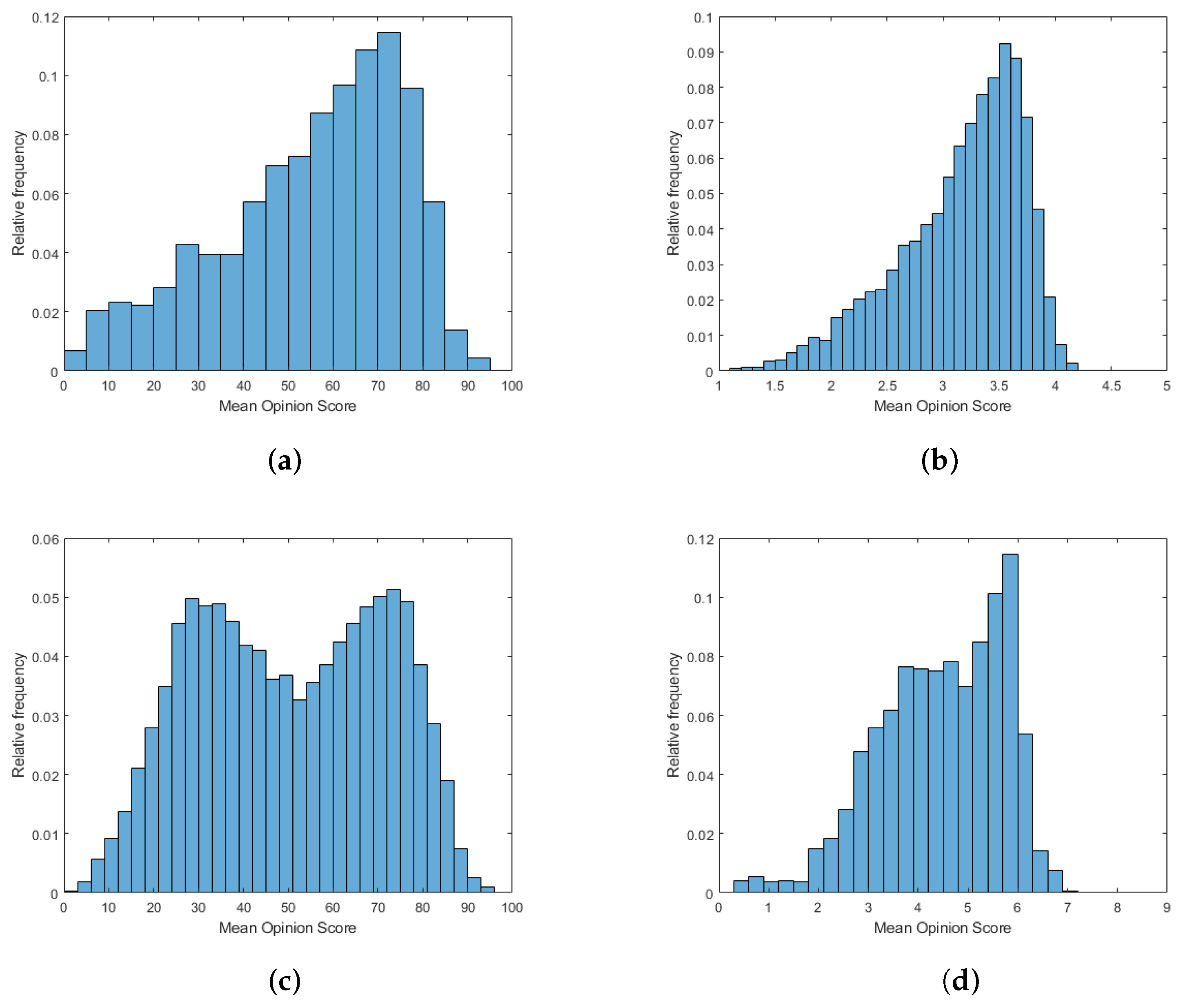
Figure 1.
MOS distributions in the applied benchmark IQA databases: (a) CLIVE [50], (b) KonIQ-10k [4], (c) SPAQ [5] and (d) TID2013 [51].

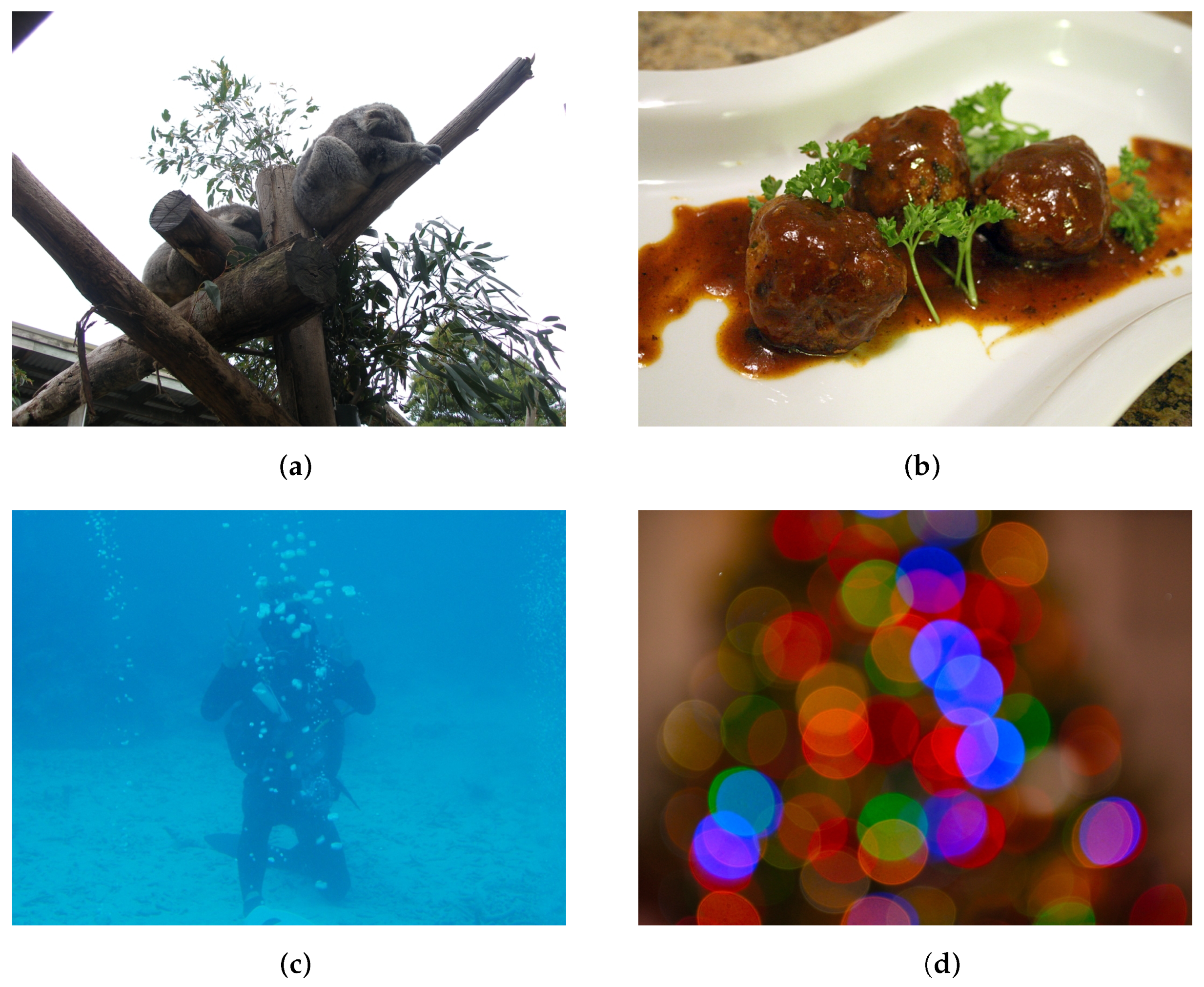
Figure 2.
Sample images from KonIQ-10k [4] with their MOS values: (a) , (b) , (c) and (d) .
Figure 2.
Sample images from KonIQ-10k [4] with their MOS values: (a) , (b) , (c) and (d) .

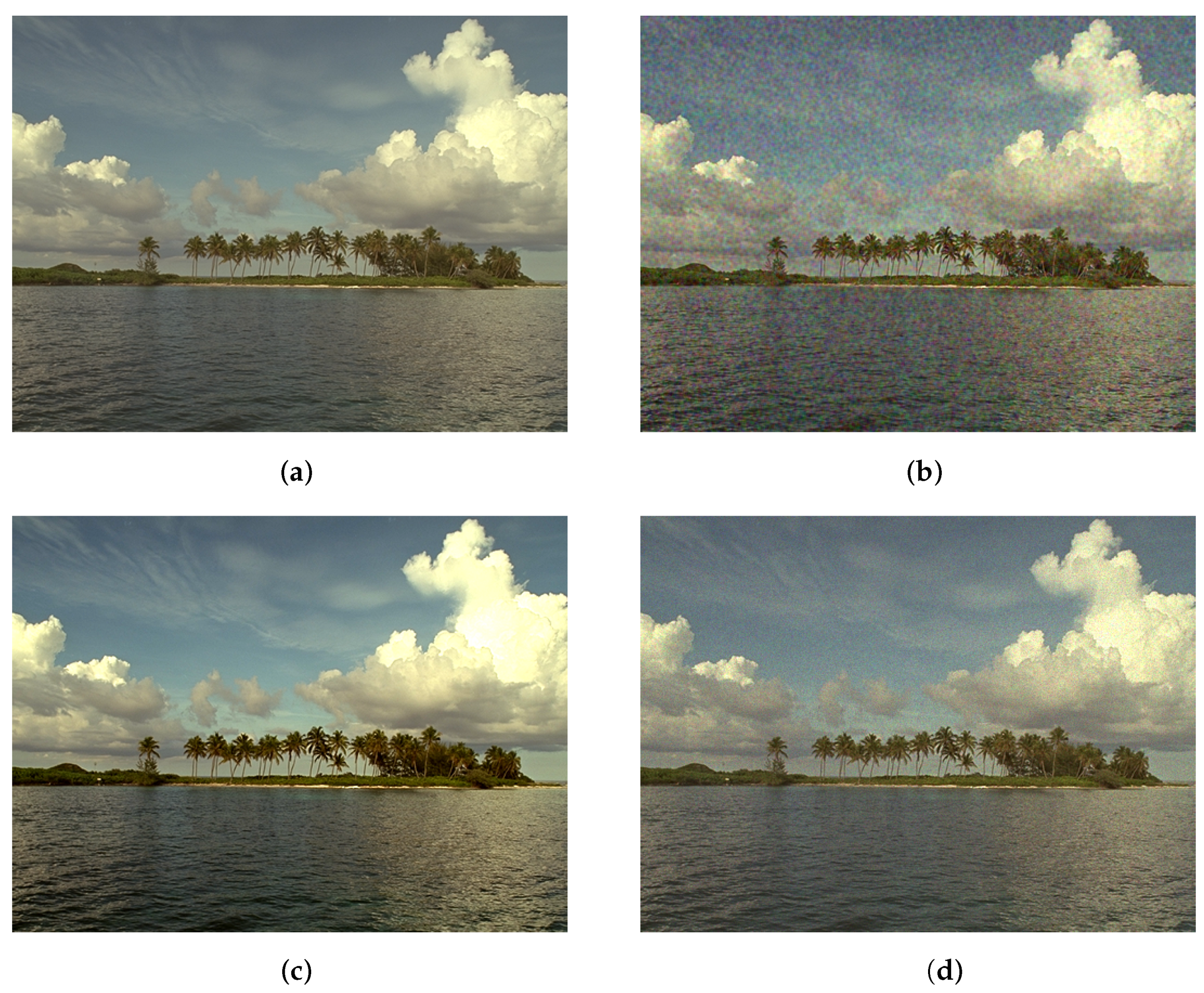
Figure 3.
Sample images from TID2013 [51] with their MOS values: (a) pristine reference image, (b) spatially correlated noise, , (c) contrast change, and (d) multiplicative Gaussian noise, .
Figure 3.
Sample images from TID2013 [51] with their MOS values: (a) pristine reference image, (b) spatially correlated noise, , (c) contrast change, and (d) multiplicative Gaussian noise, .

Figure 4.
High-level overview of the proposed method. An input image is passed through six in-parallel CNN bodies followed by global average pooling layers and regression heads. The six branches are trained using the same train and validation datasets but independently from each other. To obtain an overall quality score for the input image, the quality predictions of the six branches are fused.

Figure 5.
Illustration of global average pooling. It takes the average of each feature map to compile a new feature vector.
Figure 5.
Illustration of global average pooling. It takes the average of each feature map to compile a new feature vector.

Figure 6.
Structure of the regression head. The first three layers contains 2048, 1024 and 256 nodes with dropout rates of , and , respectively. Since the last layer predicts perceptual quality, it contains one node.
Figure 6.
Structure of the regression head. The first three layers contains 2048, 1024 and 256 nodes with dropout rates of , and , respectively. Since the last layer predicts perceptual quality, it contains one node.


Table 1.
Overview about the applied publicly available IQA benchmark databases. In this table, we denoted by ‘-’ if the data was not available.
Table 1.
Overview about the applied publicly available IQA benchmark databases. In this table, we denoted by ‘-’ if the data was not available.
| Attribute | CLIVE [50] | KonIQ-10k [4] | SPAQ [5] | TID2013 [51] |
|---|---|---|---|---|
| Year | 2015 | 2018 | 2020 | 2013 |
| Number of images | 1169 | 10,073 | 11,125 | 3000 |
| Number of scenes | 1169 | 10,073 | 11,125 | 25 |
| Distortion type | authentic | authentic | authentic | artificial |
| Subjective framework | crowd-sourcing | crowd-sourcing | laboratory | laboratory |
| Number of annotators | 8000 | 350,000 | 600 | 540 |
| Number of annotations | 1400 | 1,200,000 | 186,400 | 524,340 |
| Resolution | ∼ | |||
| MOS range | 0–100 | 1–5 | 0–100 | 0–9 |
Table 2.
On ImageNet [62] database pretrained CNNs applied in this study. In this table, Top-1 and Top-5 accuracy refers to the model’s performance on the ImageNet [55] validation dataset.
| CNN | Size (MByte) | Top-1 Accuracy | Top-5 Accuracy | Parameters | Depth |
|---|---|---|---|---|---|
| VGG16 [56] | 528 | 0.713 | 0.901 | 138,357,544 | 23 |
| ResNet50 [57] | 98 | 0.749 | 0.921 | 25,636,712 | - |
| InceptionV3 [58] | 92 | 0.779 | 0.937 | 23,851,784 | 159 |
| InceptionResNetV2 [59] | 215 | 0.803 | 0.953 | 55,873,736 | 572 |
| DenseNet201 [60] | 80 | 0.773 | 0.936 | 20,242,984 | 201 |
| NASNetMobile [61] | 23 | 0.774 | 0.919 | 5,326,716 | - |
Table 3.
Base CNN and decision fusion comparison on KonIQ-10k [4]. Median SROCC values were measured over 100 random train–validation–test splits.
Table 3.
Base CNN and decision fusion comparison on KonIQ-10k [4]. Median SROCC values were measured over 100 random train–validation–test splits.
| Architecture | SROCC |
|---|---|
| VGG16 | 0.861 |
| ResNet50 | 0.860 |
| InceptionV3 | 0.909 |
| InceptionResNetV2 | 0.918 |
| DenseNet201 | 0.914 |
| NASNetMobile | 0.899 |
| Average pooling of subscores | 0.927 |
| Median pooling of subscores | 0.931 |
Table 4.
Comparison of DF-CNN-IQA to the state of the art on CLIVE [50] and KonIQ-10k [4]. Median PLCC, SROCC and KROCC values were measured over 100 random train–validation–test splits. The best results are typed in bold, and the second-best results are underlined. We denoted by ‘-’ if the data was not available.
| CLIVE [50] | KonIQ-10k [4] | |||||
|---|---|---|---|---|---|---|
| Method | PLCC | SROCC | KROCC | PLCC | SROCC | KROCC |
| BLIINDER [66] | 0.782 | 0.763 | 0.576 | 0.876 | 0.864 | 0.668 |
| DeepRN [67] | 0.784 | 0.753 | 0.579 | 0.866 | 0.880 | 0.666 |
| BLIINDS-II [14] | 0.473 | 0.442 | 0.291 | 0.574 | 0.575 | 0.414 |
| BMPRI [68] | 0.541 | 0.487 | 0.333 | 0.637 | 0.619 | 0.421 |
| BRISQUE [15] | 0.524 | 0.497 | 0.345 | 0.707 | 0.677 | 0.494 |
| CurveletQA [11] | 0.636 | 0.621 | 0.421 | 0.730 | 0.718 | 0.495 |
| DIIVINE [9] | 0.617 | 0.580 | 0.405 | 0.709 | 0.693 | 0.471 |
| ENIQA [69] | 0.596 | 0.564 | 0.376 | 0.761 | 0.745 | 0.544 |
| GRAD-LOG-CP [70] | 0.607 | 0.604 | 0.383 | 0.705 | 0.696 | 0.501 |
| MultiGAP-NRIQA [36] | 0.841 | 0.813 | 0.626 | 0.915 | 0.911 | 0.732 |
| MSDF-IQA [40] | 0.831 | 0.801 | 0.607 | 0.901 | 0.885 | 0.703 |
| NBIQA [71] | 0.629 | 0.604 | 0.427 | 0.771 | 0.749 | 0.515 |
| PIQE [72] | 0.172 | 0.108 | 0.081 | 0.208 | 0.246 | 0.172 |
| OG-IQA [73] | 0.545 | 0.505 | 0.364 | 0.652 | 0.635 | 0.447 |
| SSEQ [74] | 0.487 | 0.436 | 0.309 | 0.589 | 0.572 | 0.423 |
| UNIQUE [75] | 0.891 | 0.855 | 0.633 | 0.900 | 0.897 | 0.664 |
| CONTRIQUE [76] | 0.857 | 0.845 | - | 0.906 | 0.894 | - |
| DB-CNN [77] | 0.869 | 0.851 | - | 0.884 | 0.875 | - |
| DeepFL-IQA [78] | 0.769 | 0.734 | - | 0.887 | 0.877 | - |
| KonCept512 [79,82] | 0.848 | 0.825 | - | 0.937 | 0.921 | - |
| MLSP [78,80] | 0.769 | 0.734 | - | 0.887 | 0.877 | - |
| PaQ-2-PiQ [46] | 0.850 | 0.840 | - | 0.880 | 0.870 | - |
| PQR [81] | 0.882 | 0.857 | - | 0.884 | 0.880 | - |
| WSP [43] | - | - | - | 0.931 | 0.918 | - |
| DF-CNN-IQA | 0.859 | 0.849 | 0.630 | 0.949 | 0.931 | 0.738 |
Table 5.
Comparison of DF-CNN-IQA to the state of the art on SPAQ [5] and TID2013 [51]. Median PLCC, SROCC and KROCC values were measured over 100 random train–validation–test splits. The best results are typed in bold, and the second-best results are underlined. We denoted by ‘-’ if the data were not available.
| SPAQ [5] | TID2013 [51] | |||||
|---|---|---|---|---|---|---|
| Method | PLCC | SROCC | KROCC | PLCC | SROCC | KROCC |
| BLIINDER [66] | 0.872 | 0.869 | 0.683 | 0.834 | 0.816 | 0.720 |
| DeepRN [67] | 0.870 | 0.850 | 0.676 | 0.745 | 0.636 | 0.560 |
| BLIINDS-II [14] | 0.676 | 0.675 | 0.486 | 0.558 | 0.513 | 0.339 |
| BMPRI [68] | 0.739 | 0.734 | 0.506 | 0.701 | 0.588 | 0.427 |
| BRISQUE [15] | 0.726 | 0.720 | 0.518 | 0.478 | 0.427 | 0.278 |
| CurveletQA [11] | 0.793 | 0.774 | 0.503 | 0.553 | 0.505 | 0.359 |
| DIIVINE [9] | 0.774 | 0.756 | 0.514 | 0.692 | 0.599 | 0.431 |
| ENIQA [69] | 0.813 | 0.804 | 0.603 | 0.604 | 0.555 | 0.397 |
| GRAD-LOG-CP [70] | 0.786 | 0.782 | 0.572 | 0.671 | 0.627 | 0.470 |
| MultiGAP-NRIQA [36] | 0.909 | 0.903 | 0.693 | 0.710 | 0.433 | 0.302 |
| MSDF-IQA [40] | 0.900 | 0.894 | 0.692 | 0.727 | 0.448 | 0.311 |
| NBIQA [71] | 0.802 | 0.793 | 0.539 | 0.723 | 0.628 | 0.427 |
| PIQE [72] | 0.211 | 0.156 | 0.091 | 0.464 | 0.365 | 0.257 |
| OG-IQA [73] | 0.726 | 0.724 | 0.594 | 0.564 | 0.452 | 0.321 |
| SSEQ [74] | 0.745 | 0.742 | 0.549 | 0.618 | 0.520 | 0.375 |
| UNIQUE [75] | 0.907 | 0.906 | 0.687 | 0.812 | 0.826 | 0.578 |
| CONTRIQUE [76] | 0.919 | 0.914 | - | 0.857 | 0.843 | - |
| DB-CNN [77] | 0.915 | 0.914 | - | 0.865 | 0.816 | - |
| DeepFL-IQA [78] | - | - | - | 0.876 | 0.858 | - |
| KonCept512 [79] | - | - | - | - | - | - |
| MLSP [78,80] | - | - | - | - | - | - |
| PaQ-2-PiQ [46] | - | - | - | - | - | - |
| PQR [81] | - | - | - | 0.798 | 0.740 | - |
| WSP [43] | - | - | - | - | - | - |
| DF-CNN-IQA | 0.921 | 0.915 | 0.693 | 0.743 | 0.709 | 0.496 |
Table 6.
Comparison of the proposed DF-CNN-IQA to the state of the art. The weighted and direct average of measured PLCC and SROCC values are reported. The best results are typed in bold, and the second-best results are underlined. We denoted by ‘-’ if the data were not available.
Table 6.
Comparison of the proposed DF-CNN-IQA to the state of the art. The weighted and direct average of measured PLCC and SROCC values are reported. The best results are typed in bold, and the second-best results are underlined. We denoted by ‘-’ if the data were not available.
| Direct Average | Weighted Average | |||||
|---|---|---|---|---|---|---|
| Method | PLCC | SROCC | KROCC | PLCC | SROCC | KROCC |
| BLIINDER [66] | 0.841 | 0.828 | 0.662 | 0.865 | 0.856 | 0.676 |
| DeepRN [67] | 0.816 | 0.780 | 0.620 | 0.850 | 0.832 | 0.654 |
| BLIINDS-II [14] | 0.570 | 0.551 | 0.383 | 0.612 | 0.605 | 0.431 |
| BMPRI [68] | 0.655 | 0.607 | 0.422 | 0.685 | 0.660 | 0.455 |
| BRISQUE [15] | 0.609 | 0.580 | 0.409 | 0.680 | 0.658 | 0.472 |
| CurveletQA [11] | 0.678 | 0.655 | 0.445 | 0.732 | 0.713 | 0.479 |
| DIIVINE [9] | 0.698 | 0.657 | 0.455 | 0.731 | 0.704 | 0.482 |
| ENIQA [69] | 0.694 | 0.667 | 0.480 | 0.758 | 0.740 | 0.545 |
| GRAD-LOG-CP [70] | 0.692 | 0.677 | 0.481 | 0.732 | 0.721 | 0.523 |
| MultiGAP-NRIQA [36] | 0.844 | 0.765 | 0.588 | 0.885 | 0.846 | 0.659 |
| MSDF-IQA [40] | 0.840 | 0.757 | 0.578 | 0.877 | 0.833 | 0.647 |
| NBIQA [71] | 0.731 | 0.694 | 0.477 | 0.772 | 0.747 | 0.511 |
| PIQE [72] | 0.264 | 0.219 | 0.150 | 0.238 | 0.214 | 0.142 |
| OG-IQA [73] | 0.622 | 0.579 | 0.432 | 0.669 | 0.646 | 0.493 |
| SSEQ [74] | 0.610 | 0.568 | 0.414 | 0.656 | 0.634 | 0.467 |
| UNIQUE [75] | 0.878 | 0.871 | 0.641 | 0.892 | 0.891 | 0.662 |
| CONTRIQUE [76] | 0.885 | 0.874 | - | 0.904 | 0.894 | - |
| DB-CNN [77] | 0.883 | 0.864 | - | 0.894 | 0.884 | - |
| DeepFL-IQA [78] | - | - | - | - | - | - |
| KonCept512 [79] | - | - | - | - | - | - |
| MLSP [78,80] | - | - | - | - | - | - |
| PaQ-2-PiQ [46] | - | - | - | - | - | - |
| PQR [81] | - | - | - | - | - | - |
| WSP [43] | - | - | - | - | - | - |
| DF-CNN-IQA | 0.868 | 0.851 | 0.639 | 0.908 | 0.894 | 0.685 |
Table 7.
Results of the one-sided t-tests. Symbol 1 (−1) means that the proposed DF-CNN-IQA method is statistically significantly confidence interval, significance level) better (worse) than the NR-IQA method in the row on the IQA benchmark database in the column.
Table 7.
Results of the one-sided t-tests. Symbol 1 (−1) means that the proposed DF-CNN-IQA method is statistically significantly confidence interval, significance level) better (worse) than the NR-IQA method in the row on the IQA benchmark database in the column.
| Method | CLIVE [50] | KonIQ-10k [4] | SPAQ [5] | TID2013 [51] |
|---|---|---|---|---|
| BLIINDER [66] | 1 | 1 | 1 | −1 |
| DeepRN [67] | 1 | 1 | 1 | 1 |
| BLIINDS-II [14] | 1 | 1 | 1 | 1 |
| BMPRI [68] | 1 | 1 | 1 | 1 |
| BRISQUE [15] | 1 | 1 | 1 | 1 |
| CurveletQA [11] | 1 | 1 | 1 | 1 |
| DIIVINE [9] | 1 | 1 | 1 | 1 |
| ENIQA [69] | 1 | 1 | 1 | 1 |
| GRAD-LOG-CP [70] | 1 | 1 | 1 | 1 |
| MultiGAP-NRIQA [36] | 1 | 1 | 1 | 1 |
| MSDF-IQA [40] | 1 | 1 | 1 | 1 |
| NBIQA [71] | 1 | 1 | 1 | 1 |
| PIQE [72] | 1 | 1 | 1 | 1 |
| OG-IQA [73] | 1 | 1 | 1 | 1 |
| SSEQ [74] | 1 | 1 | 1 | 1 |
| UNIQUE [75] | −1 | 1 | 1 | −1 |
Table 8.
Cross-database test. Methods were trained on KonIQ-10k [4] and tested on CLIVE [50]. The best results are typed in bold, and the second-best ones are underlined. We denoted by ‘-’ if the data were not available.
| Method | PLCC | SROCC | KROCC |
|---|---|---|---|
| BLIINDER [66] | 0.748 | 0.730 | 0.503 |
| DeepRN [67] | 0.746 | 0.725 | 0.481 |
| BLIINDS-II [14] | 0.107 | 0.090 | 0.063 |
| BMPRI [68] | 0.453 | 0.389 | 0.298 |
| BRISQUE [15] | 0.509 | 0.460 | 0.310 |
| CurveletQA [11] | 0.496 | 0.505 | 0.347 |
| DIIVINE [9] | 0.479 | 0.434 | 0.299 |
| ENIQA [69] | 0.428 | 0.386 | 0.272 |
| GRAD-LOG-CP [70] | 0.427 | 0.384 | 0.261 |
| MultiGAP-NRIQA [36] | 0.841 | 0.813 | 0.585 |
| MSDF-IQA [40] | 0.764 | 0.749 | 0.552 |
| NBIQA [71] | 0.503 | 0.509 | 0.284 |
| OG-IQA [73] | 0.442 | 0.427 | 0.289 |
| SSEQ [74] | 0.270 | 0.256 | 0.170 |
| UNIQUE [75] | 0.842 | 0.826 | 0.589 |
| CONTRIQUE [76] | - | 0.731 | - |
| DB-CNN [77] | - | 0.755 | - |
| DeepFL-IQA [78] | - | 0.704 | - |
| KonCept512 [79] | 0.848 | 0.825 | - |
| PaQ-2-PiQ [46] | - | - | - |
| PQR [81] | - | 0.770 | - |
| WSP [43] | 0.840 | 0.820 | - |
| DF-CNN-IQA | 0.854 | 0.831 | 0.598 |
Publisher’s Note: MDPI stays neutral with regard to jurisdictional claims in published maps and institutional affiliations. |
© 2021 by the author. Licensee MDPI, Basel, Switzerland. This article is an open access article distributed under the terms and conditions of the Creative Commons Attribution (CC BY) license (https://creativecommons.org/licenses/by/4.0/).
Share and Cite
MDPI and ACS Style
Varga, D. No-Reference Image Quality Assessment with Convolutional Neural Networks and Decision Fusion. Appl. Sci. 2022, 12, 101. https://doi.org/10.3390/app12010101
AMA Style
Varga D. No-Reference Image Quality Assessment with Convolutional Neural Networks and Decision Fusion. Applied Sciences. 2022; 12(1):101. https://doi.org/10.3390/app12010101
Chicago/Turabian StyleVarga, Domonkos. 2022. "No-Reference Image Quality Assessment with Convolutional Neural Networks and Decision Fusion" Applied Sciences 12, no. 1: 101. https://doi.org/10.3390/app12010101
Note that from the first issue of 2016, this journal uses article numbers instead of page numbers. See further details here.