
Analytical Modeling of Current-Voltage Photovoltaic Performance: An Easy Approach to Solar Panel Behavior


 , ,
, ,  ,
,
Abstract
:1. Introduction
- The extraction of the parameters appearing in this equation, which define the performance of the photovoltaic device at a certain temperature and irradiance level, and;
- The calculation of the output current as a function of the output voltage, or vice versa, since this equation is implicit.
- Selection of a proper ideality factor for extraction of the model parameters based on analytical methods, as this forms the cornerstone for extracting the other four parameters [57], and;
- Development of a simplified approach to the Lambert W-function, which is required in this analytical methodology in order to:
- ○
- Obtain the value of the first parameter of the 1-D/2-R equivalent circuit model, i.e., the value of the resistance of the series-connected resistor, and;
- ○
- Solve the implicit equation of this model to derive the output current in relation to the output voltage.
2. Modeling of Photovoltaic Systems
2.1. The 1-D/2-R Equivalent Circuit Model
- The I-V curve with an enough large number of points, or;
- The three characteristic points of the I-V curve (short circuit output current, Isc, open circuit output voltage, Voc, and output current and voltage levels at the Maximum Power Point (MPP), Imp and Vmp,
- A sufficiently accurate estimation of the ideality factor a is required;
- Equation (4) is an implicit mathematical expression for solving Rs, and an iterative process is, therefore, required to extract this parameter; and
- Equation (1), which defines the performance of the solar cell/panel, is also an implicit expression. As a consequence, once all the parameters of this equation have been extracted, an additional iterative process will be required to solve it (i.e., to derive the value of the output current, I, for a given value of the output voltage level, V).
2.2. Explicit Equations/Models as Alternative to the 1-D/2-R Equivalent Circuit Model
2.3. The Lambert W-Function
- W0(x), for W(x) ≥ −1, and
- W−1(x), for W(x) ≤ −1.
3. Results
- Sub-Section 3.1 describes the problem of selecting a suitable value for the ideality factor, a, in order to obtain the values for the rest of the parameters.
- Very simple equations for the Lambert W-function, for use in solving the equations described in the section above, are included in Sub-Section 3.2.
- Finally, a case study in which our methodologies are applied to the modeling of spacecraft solar panels is included in Sub-Section 3.3.
3.1. On the Best Value for the Ideality Factor
- Rs was calculated using Equation (8) to (12);
- Rsh was calculated using Equation (5);
- Ipv was calculated using Equation (6);
- I0 was calculated using Equation (7).
- The analytical methodology suggested in the present work may give unacceptable results when the ideality factor exceeds a certain value, as complex numbers start to emerge in the calculations.
- One of the parameters obtained analytically for the best fit in terms of the non-dimensional RMSE has no physical meaning: this is the negative value of the resistance of the shunt resistor shown in Table 3, which is obtained for the Photowatt PWP 201 solar panel.
3.2. Lambert W-Function Simplified Equations for Solar Cell/Panel Modeling
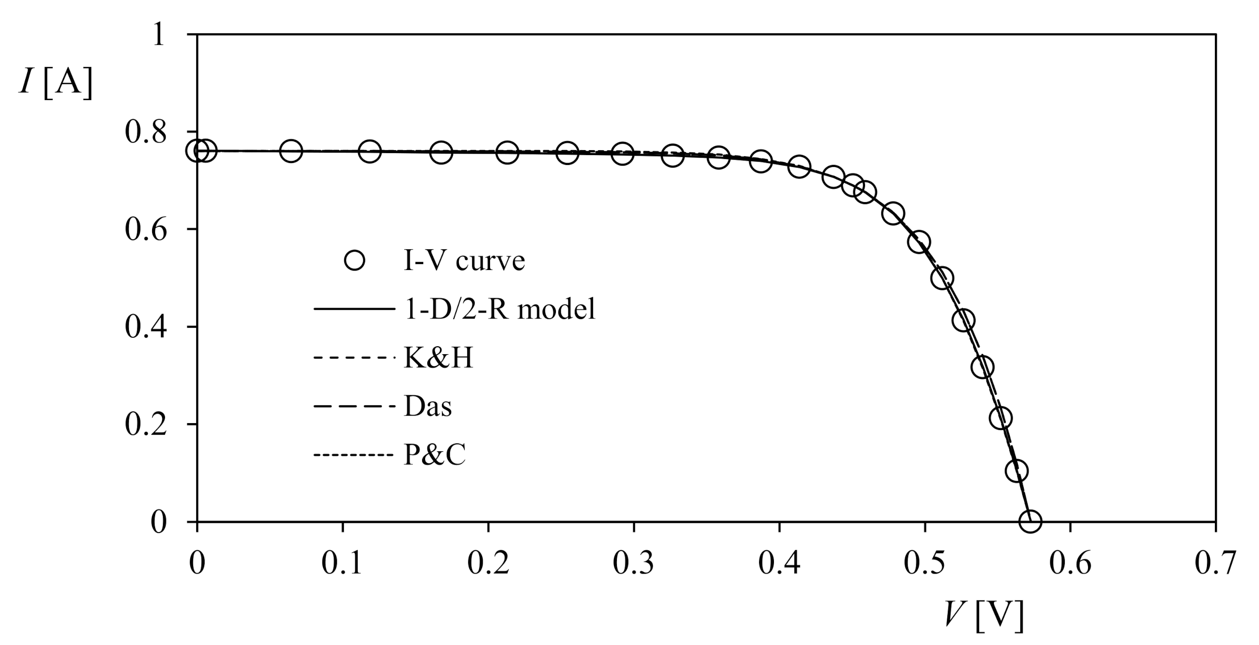
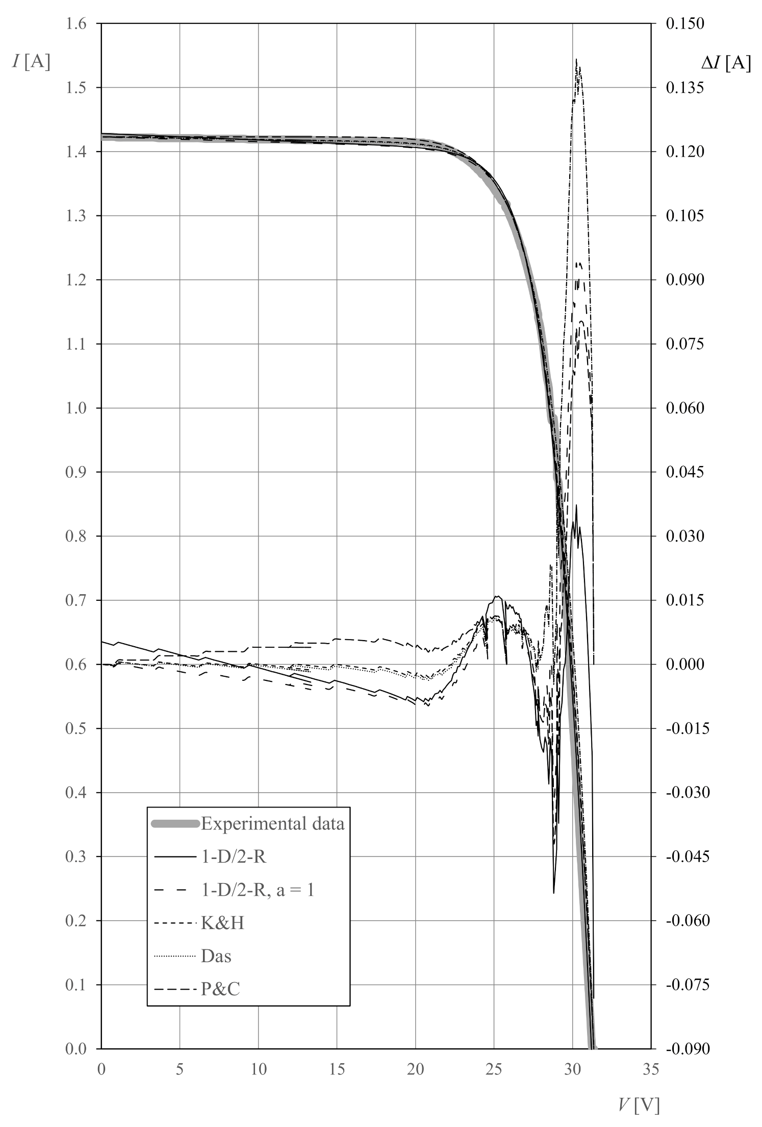
3.3. Case Study: The Solar Panels of the UPMSat-1
- The best fit of the 1-D/2-R equivalent circuit model (see Table 6);
- The analytical fit for a = 1 (Equations (5–12)), and our approximations to the Lambert W-function (Equations (26)–(28),(31,32));
- The explicit models proposed by Kalmarkar and Haneefa, Das (Equations (14)–(20), (35,36)), and Pindado and Cubas (Equations (21) and (22)), see Table 7.
4. Conclusions
- An initial estimation of the ideality factor, a, is required.
- The equation for the value of the resistance of the series-connected resistor, Rs, is an implicit expression, meaning that either an iterative process or the Lambert W-function is required.
- When all the parameters for the 1-D/2-R equivalent circuit model have been extracted, an implicit equation must be solved (or the Lambert W-function must be used) to derive the value of the output current for a given output voltage.
- The use of the Lambert W-function requires some numerical and calculation resources and skills.
- The use of explicit models rather than the 1-D/2-R equivalent circuit model, in order to avoid the problems described above, may not be possible, as some of them require the Lambert W-function to derive their parameters, based on the characteristic points of the I-V curve.
- A value of a = 1 for the 1-D/2-R equivalent circuit model was shown to be reasonable for most photovoltaic technologies.
- The analytical procedure for extracting the parameters for the 1-D/2-R equivalent circuit model may give values for the resistance of one resistor (or even both) that are negative. However, this does not affect the results (i.e., the modeled performance of the photovoltaic device).
- The Lambert W-function can be simplified for use in modeling the performance of photovoltaic devices. Accurate simplified versions of the Lambert W-function are proposed here for three cases, depending on the specific need: (i) calculation of Rs; (ii) calculation of the output current using the equation for the 1-D/2-R equivalent circuit; or (iii) calculation of the parameters for certain explicit models.
- Explicit models are also accurate alternatives to the 1-D/2-R equivalent circuit model.
Author Contributions
Funding
Institutional Review Board Statement
Informed Consent Statement
Data Availability Statement
Acknowledgments
Conflicts of Interest
Appendix A. Approximation to the Right-Side of the Lambert W-Function Positive Branch by Larry et al. (2000) (see References)
Appendix B. I-V Curves of the UPMSat-1 Solar Panels.

| V [V] | I [A] | V [V] | I [A] | V [V] | I [A] | V [V] | I [A] | V [V] | I [A] | V [V] | I [A] |
|---|---|---|---|---|---|---|---|---|---|---|---|
| −0.950 | 1.431 | 5.189 | 1.430 | 10.813 | 1.429 | 16.204 | 1.428 | 21.510 | 1.418 | 26.428 | 1.213 |
| −0.801 | 1.431 | 5.330 | 1.430 | 10.944 | 1.429 | 13.338 | 1.428 | 21.632 | 1.417 | 26.545 | 1.198 |
| −0.660 | 1.431 | 5.471 | 1.430 | 11.077 | 1.429 | 16.459 | 1.428 | 21.758 | 1.416 | 26.657 | 1.182 |
| −0.510 | 1.431 | 5.613 | 1.430 | 11.217 | 1.429 | 16.589 | 1.427 | 21.879 | 1.415 | 26.775 | 1.165 |
| −0.370 | 1.431 | 5.744 | 1.430 | 11.348 | 1.429 | 16.723 | 1.427 | 22.001 | 1.414 | 26.887 | 1.148 |
| −0.221 | 1.431 | 5.888 | 1.430 | 11.480 | 1.429 | 16.848 | 1.427 | 22.128 | 1.413 | 27.006 | 1.129 |
| −0.079 | 1.431 | 6.026 | 1.430 | 11.614 | 1.429 | 16.980 | 1.427 | 22.248 | 1.412 | 27.118 | 1.110 |
| 0.067 | 1.431 | 6.167 | 1.430 | 11.745 | 1.429 | 17.101 | 1.427 | 22.372 | 1.411 | 27.226 | 1.090 |
| 0.210 | 1.431 | 6.309 | 1.430 | 11.885 | 1.429 | 17.234 | 1.427 | 22.493 | 1.409 | 27.343 | 1.068 |
| 0.360 | 1.431 | 6.440 | 1.430 | 12.019 | 1.429 | 17.388 | 1.427 | 22.617 | 1.408 | 27.453 | 1.048 |
| 0.600 | 1.431 | 6.580 | 1.430 | 12.149 | 1.429 | 17.489 | 1.427 | 22.741 | 1.406 | 27.572 | 1.021 |
| 0.660 | 1.431 | 6.727 | 1.430 | 12.282 | 1.429 | 17.621 | 1.427 | 22.861 | 1.405 | 27.681 | 0.997 |
| 0.782 | 1.431 | 6.863 | 1.430 | 12.413 | 1.429 | 17.744 | 1.427 | 22.987 | 1.403 | 27.789 | 0.972 |
| 0.924 | 1.431 | 6.983 | 1.429 | 12.545 | 1.428 | 17.999 | 1.427 | 23.099 | 1.401 | 27.908 | 0.943 |
| 1.071 | 1.431 | 7.136 | 1.429 | 12.678 | 1.428 | 18.122 | 1.427 | 23.221 | 1.399 | 28.013 | 0.916 |
| 1.214 | 1.430 | 7.277 | 1.429 | 12.810 | 1.428 | 18.253 | 1.426 | 23.343 | 1.396 | 28.122 | 0.888 |
| 1.364 | 1.430 | 7.407 | 1.429 | 12.942 | 1.428 | 18.278 | 1.426 | 23.485 | 1.394 | 28.230 | 0.858 |
| 1.503 | 1.430 | 7.546 | 1.429 | 13.075 | 1.428 | 18.510 | 1.426 | 23.588 | 1.391 | 28.345 | 0.825 |
| 1.643 | 1.430 | 7.689 | 1.429 | 13.206 | 1.428 | 18.635 | 1.426 | 23.712 | 1.388 | 28.483 | 0.793 |
| 1.786 | 1.430 | 7.822 | 1.429 | 13.336 | 1.428 | 18.756 | 1.426 | 23.827 | 1.385 | 28.558 | 0.761 |
| 1.936 | 1.430 | 7.963 | 1.429 | 13.470 | 1.428 | 18.889 | 1.426 | 23.948 | 1.381 | 28.665 | 0.727 |
| 2.076 | 1.430 | 8.094 | 1.429 | 13.601 | 1.428 | 19.011 | 1.426 | 24.071 | 1.378 | 28.780 | 0.689 |
| 2.216 | 1.430 | 8.235 | 1.429 | 13.734 | 1.428 | 19.138 | 1.426 | 24.183 | 1.374 | 28.884 | 0.653 |
| 2.367 | 1.430 | 8.374 | 1.429 | 13.884 | 1.428 | 19.267 | 1.425 | 24.305 | 1.370 | 28.992 | 0.615 |
| 2.508 | 1.430 | 8.507 | 1.429 | 13.997 | 1.428 | 19.390 | 1.425 | 24.427 | 1.365 | 29.096 | 0.577 |
| 2.648 | 1.430 | 8.648 | 1.429 | 14.129 | 1.428 | 19.514 | 1.425 | 24.550 | 1.360 | 29.200 | 0.538 |
| 2.709 | 1.430 | 8.780 | 1.429 | 14.262 | 1.428 | 19.648 | 1.425 | 24.671 | 1.354 | 29.314 | 0.494 |
| 2.930 | 1.430 | 8.923 | 1.429 | 14.392 | 1.428 | 19.769 | 1.424 | 24.784 | 1.349 | 29.420 | 0.452 |
| 3.068 | 1.430 | 9.053 | 1.429 | 14.515 | 1.428 | 19.892 | 1.424 | 24.905 | 1.343 | 29.524 | 0.410 |
| 3.219 | 1.430 | 9.194 | 1.429 | 14.649 | 1.428 | 20.016 | 1.424 | 25.027 | 1.338 | 29.629 | 0.366 |
| 3.359 | 1.430 | 9.325 | 1.429 | 14.780 | 1.428 | 20.146 | 1.424 | 25.139 | 1.329 | 29.738 | 0.320 |
| 3.500 | 1.430 | 9.456 | 1.429 | 14.911 | 1.428 | 20.263 | 1.423 | 25.261 | 1.322 | 29.847 | 0.271 |
| 3.642 | 1.430 | 9.598 | 1.429 | 15.042 | 1.428 | 20.395 | 1.423 | 25.377 | 1.314 | 29.960 | 0.220 |
| 4.064 | 1.430 | 9.730 | 1.429 | 15.168 | 1.428 | 20.518 | 1.422 | 25.496 | 1.305 | 30.074 | 0.167 |
| 4.204 | 1.430 | 9.870 | 1.429 | 16.297 | 1.428 | 20.639 | 1.422 | 25.617 | 1.296 | 30.189 | 0.113 |
| 4.347 | 1.430 | 10.003 | 1.429 | 15.430 | 1.428 | 20.762 | 1.422 | 25.729 | 1.286 | 30.299 | 0.067 |
| 4.485 | 1.430 | 10.136 | 1.429 | 15.561 | 1.428 | 20.896 | 1.421 | 25.848 | 1.278 | 30.409 | 0.018 |
| 4.628 | 1.430 | 10.275 | 1.429 | 15.666 | 1.428 | 21.018 | 1.421 | 25.961 | 1.265 | 30.513 | 0.000 |
| 4.767 | 1.430 | 10.407 | 1.429 | 15.815 | 1.428 | 21.140 | 1.420 | 26.082 | 1.253 | ||
| 4.909 | 1.430 | 10.540 | 1.429 | 15.949 | 1.428 | 21.265 | 1.419 | 26.193 | 1.241 | ||
| 5.047 | 1.430 | 10.661 | 1.429 | 16.082 | 1.428 | 21.388 | 1.419 | 26.314 | 1.227 |
| V [V] | I [A] | V [V] | I [A] | V [V] | I [A] | V [V] | I [A] | V [V] | I [A] | V [V] | I [A] |
|---|---|---|---|---|---|---|---|---|---|---|---|
| −0.638 | 1.423 | 9.402 | 1.419 | 19.166 | 1.416 | 22.469 | 1.399 | 25.814 | 1.310 | 28.142 | 1.093 |
| −0.518 | 1.423 | 9.722 | 1.419 | 19.269 | 1.416 | 22.593 | 1.398 | 25.844 | 1.309 | 28.249 | 1.069 |
| −0.198 | 1.423 | 10.042 | 1.419 | 19.373 | 1.416 | 22.687 | 1.396 | 25.917 | 1.305 | 28.367 | 1.047 |
| 0.122 | 1.423 | 10.362 | 1.419 | 19.476 | 1.415 | 22.801 | 1.395 | 25.990 | 1.300 | 28.485 | 1.031 |
| 0.442 | 1.423 | 10.882 | 1.419 | 19.560 | 1.415 | 22.905 | 1.393 | 26.063 | 1.296 | 28.581 | 0.999 |
| 0.782 | 1.423 | 11.002 | 1.419 | 19.684 | 1.415 | 23.009 | 1.391 | 26.136 | 1.292 | 28.680 | 0.980 |
| 1.082 | 1.422 | 13.322 | 1.419 | 19.788 | 1.415 | 23.113 | 1.390 | 26.209 | 1.287 | 28.795 | 0.984 |
| 1.402 | 1.422 | 11.842 | 1.419 | 19.892 | 1.415 | 23.217 | 1.388 | 26.282 | 1.283 | 28.990 | 0.923 |
| 1.722 | 1.422 | 11.962 | 1.419 | 19.986 | 1.415 | 23.320 | 1.386 | 26.365 | 1.278 | 29.007 | 0.892 |
| 2.042 | 1.422 | 12.282 | 1.418 | 20.100 | 1.414 | 23.424 | 1.384 | 26.428 | 1.273 | 29.112 | 0.883 |
| 2.362 | 1.422 | 12.602 | 1.418 | 20.204 | 1.414 | 23.528 | 1.382 | 26.500 | 1.268 | 29.216 | 0.828 |
| 2.882 | 1.422 | 12.922 | 1.418 | 20.308 | 1.414 | 23.632 | 1.380 | 26.573 | 1.262 | 29.321 | 0.793 |
| 3.002 | 1.422 | 13.242 | 1.418 | 20.411 | 1.414 | 23.736 | 1.377 | 26.646 | 1.257 | 29.424 | 0.753 |
| 3.322 | 1.422 | 13.682 | 1.418 | 20.515 | 1.414 | 23.840 | 1.375 | 26.718 | 1.251 | 29.527 | 0.718 |
| 3.642 | 1.421 | 13.882 | 1.418 | 20.619 | 1.413 | 23.944 | 1.372 | 26.792 | 1.248 | 29.630 | 0.678 |
| 3.882 | 1.421 | 14.202 | 1.418 | 20.723 | 1.413 | 24.048 | 1.370 | 26.865 | 1.240 | 29.732 | 0.632 |
| 4.282 | 1.421 | 14.522 | 1.418 | 20.827 | 1.413 | 24.152 | 1.367 | 26.938 | 1.234 | 29.834 | 0.589 |
| 4.602 | 1.421 | 14.842 | 1.417 | 20.931 | 1.412 | 24.265 | 1.364 | 27.011 | 1.227 | 29.935 | 0.543 |
| 4.922 | 1.421 | 15.162 | 1.417 | 21.035 | 1.412 | 24.590 | 1.362 | 27.084 | 1.221 | 30.035 | 0.502 |
| 5.242 | 1.421 | 15.482 | 1.417 | 21.139 | 1.411 | 24.483 | 1.359 | 27.157 | 1.214 | 30.138 | 0.465 |
| 5.562 | 1.421 | 15.802 | 1.417 | 21.243 | 1.410 | 24.567 | 1.356 | 27.230 | 1.207 | 30.239 | 0.416 |
| 5.882 | 1.421 | 16.122 | 1.417 | 21.248 | 1.410 | 24.671 | 1.352 | 27.303 | 1.200 | 30.344 | 0.382 |
| 6.202 | 1.421 | 16.442 | 1.417 | 21.450 | 1.409 | 24.776 | 1.349 | 27.378 | 1.193 | 30.455 | 0.329 |
| 6.622 | 1.420 | 16.762 | 1.417 | 21.554 | 1.408 | 24.879 | 1.346 | 27.448 | 1.186 | 30.568 | 0.282 |
| 6.842 | 1.420 | 17.082 | 1.417 | 21.668 | 1.408 | 24.983 | 1.342 | 27.521 | 1.178 | 30.682 | 0.234 |
| 7.182 | 1.420 | 17.402 | 1.417 | 21.762 | 1.407 | 25.087 | 1.338 | 27.594 | 1.170 | 30.797 | 0.187 |
| 7.482 | 1.420 | 17.722 | 1.416 | 21.868 | 1.406 | 25.180 | 1.335 | 27.687 | 1.163 | 30.911 | 0.139 |
| 7.802 | 1.420 | 18.042 | 1.416 | 21.970 | 1.405 | 25.284 | 1.331 | 27.740 | 1.154 | 31.021 | 0.094 |
| 8.122 | 1.420 | 18.362 | 1.416 | 22.074 | 1.404 | 25.398 | 1.327 | 27.813 | 1.146 | 31.131 | 0.048 |
| 8.442 | 1.420 | 18.682 | 1.416 | 22.178 | 1.403 | 25.502 | 1.323 | 27.805 | 1.141 | 31.241 | 0.002 |
| 8.762 | 1.420 | 19.002 | 1.416 | 22.282 | 1.402 | 25.806 | 1.318 | 27.916 | 1.130 | 31.351 | 0.000 |
| 9.082 | 1.420 | 19.061 | 1.416 | 22.386 | 1.400 | 25.710 | 1.314 | 28.032 | 1.112 |
References
- IEA. Technology Roadmap-Solar Photovoltaic Energy 2014; IEA: Paris, France, 2014. [Google Scholar]
- Jäger-Waldau, A. Snapshot of photovoltaics February 2018. EPJ Photovolt. 2018, 9, 6. [Google Scholar] [CrossRef]
- Zafrilla Rodríguez, J.E.; Arce Gonzalez, G.; Cadarso Vecina, M.Á.; Córcoles Fuentes, C.; Gómez Sanz, N.; López Santiago, L.A.; Monsalve Serrano, F.; Tobarra Gómez, M.Á. El Desarrollo Actual de la Energía Solar Fotovoltaica en España; Universidad de Murcia: Murcia, Spain, 2018. [Google Scholar]
- Pandey, A.; Tyagi, V.; Selvaraj, J.A.; Rahim, N.; Tyagi, S. Recent advances in solar photovoltaic systems for emerging trends and advanced applications. Renew. Sustain. Energy Rev. 2016, 53, 859–884. [Google Scholar] [CrossRef]
- Sommerfeld, J.; Buys, L.; Vine, D. Residential consumers’ experiences in the adoption and use of solar PV. Energy Policy 2017, 105, 10–16. [Google Scholar] [CrossRef] [Green Version]
- Hussain, A.; Arif, S.M.; Aslam, M. Emerging renewable and sustainable energy technologies: State of the art. Renew. Sustain. Energy Rev. 2017, 71, 12–28. [Google Scholar] [CrossRef]
- Ueckerdt, F.; Brecha, R.; Luderer, G. Analyzing major challenges of wind and solar variability in power systems. Renew. Energy 2015, 81, 1–10. [Google Scholar] [CrossRef]
- Kylili, A.; Fokaides, P.A.; Ioannides, A.; Kalogirou, S. Environmental assessment of solar thermal systems for the industrial sector. J. Clean. Prod. 2018, 176, 99–109. [Google Scholar] [CrossRef]
- Kannan, N.; Vakeesan, D. Solar energy for future world—A review. Renew. Sustain. Energy Rev. 2016, 62, 1092–1105. [Google Scholar] [CrossRef]
- Abolhosseini, S.; Heshmati, A. The main support mechanisms to finance renewable energy development. Renew. Sustain. Energy Rev. 2014, 40, 876–885. [Google Scholar] [CrossRef] [Green Version]
- Zahedi, A. Solar photovoltaic (PV) energy; latest developments in the building integrated and hybrid PV systems. Renew. Energy 2006, 31, 711–718. [Google Scholar] [CrossRef]
- Rauschenbach, H.S. Solar Cell Array Design Handbook; J.B. Metzler: Berlin, Germany, 1980. [Google Scholar]
- Bandecchi, M.; Melton, B.; Ongaro, F. Concurrent engineering applied to space mission assessment and design. ESA Bull. Sp. Agency 1999, 99, 34–40. [Google Scholar]
- Wall, S.D. Use of Concurrent Engineering in Space Mission Design. In Proceedings of the 2nd European Systems Engineering Conference (EuSEC), Munich, Germany, 13–15 September 2000; pp. 1–6. [Google Scholar]
- Braukhane, A.; Quantius, D. Interactions in space systems design within a Concurrent Engineering facility. In Proceedings of the 2011 International Conference on Collaboration Technologies and Systems (CTS), Philadelphia, PA, USA, 23–27 May 2011; pp. 381–388. [Google Scholar]
- Ivanov, A.B.; Masson, L.; Belloni, F. Operation of a Concurrent Design Facility for university projects. In Proceedings of the 2016 IEEE Aerospace Conference, Big Sky, MT, USA, 5–12 March 2016; pp. 1–9. [Google Scholar]
- Loureiro, G.; Panades, W.; Silva, A. Lessons learned in 20 years of application of Systems Concurrent Engineering to space products. Acta Astronaut. 2018, 151, 44–52. [Google Scholar] [CrossRef]
- Ballesteros, J.B.; Alvarez, J.M.; Arcenillas, P.; Roibas, E.; Cubas, J.; Pindado, S. CDF as a tool for space engineering master’s student collaboration and concurrent design learning. In Proceedings of the 8th International Workshop on System & Concurrent Engineering for Space Applications (SECESA 2018), Glasgow, UK, 26–28 September 2018. [Google Scholar]
- Roibás-Millán, E.; Sorribes-Palmer, F.; Chimeno-Manguán, M. The MEOW lunar project for education and science based on concurrent engineering approach. Acta Astronaut. 2018, 148, 111–120. [Google Scholar] [CrossRef]
- Cotfas, D.; Cotfas, P.; Kaplanis, S. Methods to determine the dc parameters of solar cells: A critical review. Renew. Sustain. Energy Rev. 2013, 28, 588–596. [Google Scholar] [CrossRef]
- Ortiz-Conde, A.; García-Sánchez, F.J.; Muci, J.; Sucre-González, A. A review of diode and solar cell equivalent circuit model lumped parameter extraction procedures. Facta Univ. Ser. Electron. Energetics 2014, 27, 57–102. [Google Scholar] [CrossRef]
- Jena, D.; Ramana, V.V. Modeling of photovoltaic system for uniform and non-uniform irradiance: A critical review. Renew. Sustain. Energy Rev. 2015, 52, 400–417. [Google Scholar] [CrossRef]
- Chin, V.J.; Salam, Z.; Ishaque, K. Cell modelling and model parameters estimation techniques for photovoltaic simulator application: A review. Appl. Energy 2015, 154, 500–519. [Google Scholar] [CrossRef]
- Humada, A.M.; Hojabri, M.; Mekhilef, S.; Hamada, H.M. Solar cell parameters extraction based on single and double-diode models: A review. Renew. Sustain. Energy Rev. 2016, 56, 494–509. [Google Scholar] [CrossRef] [Green Version]
- Ibrahim, H.; Anani, N. Evaluation of Analytical Methods for Parameter Extraction of PV modules. Energy Procedia 2017, 134, 69–78. [Google Scholar] [CrossRef]
- Abbassi, R.; Abbassi, A.; Jemli, M.; Chebbi, S. Identification of unknown parameters of solar cell models: A comprehensive overview of available approaches. Renew. Sustain. Energy Rev. 2018, 90, 453–474. [Google Scholar] [CrossRef]
- Bader, S.; Ma, X.; Oelmann, B. One-diode photovoltaic model parameters at indoor illumination levels-A comparison. Sol. Energy 2019, 180, 707–716. [Google Scholar] [CrossRef]
- Yang, X.; Gong, W.; Wang, L. Comparative study on parameter extraction of photovoltaic models via differential evolution. Energy Convers. Manag. 2019, 201, 112113. [Google Scholar] [CrossRef]
- Oulcaid, M.; El Fadil, H.; Ammeh, L.; Yahya, A.; Giri, F. Parameter extraction of photovoltaic cell and module: Analysis and discussion of various combinations and test cases. Sustain. Energy Technol. Assess. 2020, 40, 100736. [Google Scholar] [CrossRef]
- Zhang, Y.; Ma, M.; Jin, Z. Comprehensive learning Jaya algorithm for parameter extraction of photovoltaic models. Energy 2020, 211, 118644. [Google Scholar] [CrossRef]
- Li, S.; Gu, Q.; Gong, W.; Ning, B. An enhanced adaptive differential evolution algorithm for parameter extraction of photovoltaic models. Energy Convers. Manag. 2020, 205. [Google Scholar] [CrossRef]
- Ben Messaoud, R. Extraction of uncertain parameters of a single-diode model for a photovoltaic panel using lightning attachment procedure optimization. J. Comput. Electron. 2020, 19, 1192–1202. [Google Scholar] [CrossRef]
- Ridha, H.M.; Gomes, C.; Hizam, H. Estimation of photovoltaic module model’s parameters using an improved electromagnetic-like algorithm. Neural Comput. Appl. 2020, 32, 12627–12642. [Google Scholar] [CrossRef]
- Luu, T.V.; Nguyen, N.S. Parameters extraction of solar cells using modified JAYA algorithm. Optics 2020, 203, 164034. [Google Scholar] [CrossRef]
- Abdulrazzaq, A.K.; Bognár, G.; Plesz, B. Evaluation of different methods for solar cells/modules parameters extraction. Sol. Energy 2020, 196, 183–195. [Google Scholar] [CrossRef]
- Gude, S.; Jana, K.C. Parameter extraction of photovoltaic cell using an improved cuckoo search optimization. Sol. Energy 2020, 204, 280–293. [Google Scholar] [CrossRef]
- Yousri, D.; Thanikanti, S.B.; Allam, D.; Ramachandaramurthy, V.K.; Eteiba, M. Fractional chaotic ensemble particle swarm optimizer for identifying the single, double, and three diode photovoltaic models’ parameters. Energy 2020, 195, 116979. [Google Scholar] [CrossRef]
- Diab, A.A.Z.; Sultan, H.M.; Do, T.D.; Kamel, O.M.; Mossa, M.A. Coyote Optimization Algorithm for Parameters Estimation of Various Models of Solar Cells and PV Modules. IEEE Access 2020, 8, 111102–111140. [Google Scholar] [CrossRef]
- Liang, J.; Ge, S.; Qu, B.; Yu, K.; Liu, F.; Yang, H.; Wei, P.; Li, Z. Classified perturbation mutation based particle swarm optimization algorithm for parameters extraction of photovoltaic models. Energy Convers. Manag. 2020, 203, 112138. [Google Scholar] [CrossRef]
- Liang, J.; Qiao, K.; Yuan, M.; Yu, K.; Qu, B.; Ge, S.; Li, Y.; Chen, G. Evolutionary multi-task optimization for parameters extraction of photovoltaic models. Energy Convers. Manag. 2020, 207, 112509. [Google Scholar] [CrossRef]
- Long, W.; Cai, S.; Jiao, J.; Xu, M.; Wu, T. A new hybrid algorithm based on grey wolf optimizer and cuckoo search for parameter extraction of solar photovoltaic models. Energy Convers. Manag. 2020, 203, 112243. [Google Scholar] [CrossRef]
- Ridha, H.M.; Heidari, A.A.; Wang, M.; Chen, H. Boosted mutation-based Harris hawks optimizer for parameters identification of single-diode solar cell models. Energy Convers. Manag. 2020, 209, 112660. [Google Scholar] [CrossRef]
- Xiong, G.; Zhang, J.; Shi, D.; Zhu, L.; Yuan, X.; Tan, Z. Winner-leading competitive swarm optimizer with dynamic Gaussian mutation for parameter extraction of solar photovoltaic models. Energy Convers. Manag. 2020, 206, 112450. [Google Scholar] [CrossRef]
- Zhang, Y.; Jin, Z.; Mirjalili, S. Generalized normal distribution optimization and its applications in parameter extraction of photovoltaic models. Energy Convers. Manag. 2020, 224, 113301. [Google Scholar] [CrossRef]
- Montano, J.; Tobón, A.F.; Villegas, J.P.; Durango, M. Grasshopper optimization algorithm for parameter estimation of photovoltaic modules based on the single diode model. Int. J. Energy Environ. Eng. 2020, 11, 367–375. [Google Scholar] [CrossRef]
- Ramadan, A.; Kamel, S.; Korashy, A.; Yu, J. Photovoltaic Cells Parameter Estimation Using an Enhanced Teaching–Learning-Based Optimization Algorithm. Iran. J. Sci. Technol. Trans. Electr. Eng. 2019, 44, 767–779. [Google Scholar] [CrossRef]
- Benahmida, A.; Maouhoub, N.; Sahsah, H. An Efficient Iterative Method for Extracting Parameters of Photovoltaic Panels with Single Diode Model. In Proceedings of the 2020 5th International Conference on Renewable Energies for Developing Countries (REDEC), Marrakech, Morocco, 29–30 June 2020; pp. 1–6. [Google Scholar]
- Ndegwa, R.; Simiyu, J.; Ayieta, E.; Odero, N. A Fast and Accurate Analytical Method for Parameter Determination of a Photovoltaic System Based on Manufacturer’s Data. J. Renew. Energy 2020, 2020, 1–18. [Google Scholar] [CrossRef]
- Arabshahi, M.; Torkaman, H.; Keyhani, A. A method for hybrid extraction of single-diode model parameters of photovoltaics. Renew. Energy 2020, 158, 236–252. [Google Scholar] [CrossRef]
- Peng, L.; Sun, Y.; Meng, Z.; Wang, Y.; Xu, Y. A new method for determining the characteristics of solar cells. J. Power Sources 2013, 227, 131–136. [Google Scholar] [CrossRef]
- Batzelis, E.I.; Anagnostou, G.; Chakraborty, C.; Pal, B.C. Computation of the Lambert W Function in Photovoltaic Modeling. In Lecture Notes in Electrical Engineering; J.B. Metzler: Berlin, Germany, 2020; pp. 583–595. [Google Scholar]
- Yu, F.; Huang, G.; Xu, C. An explicit method to extract fitting parameters in lumped-parameter equivalent circuit model of industrial solar cells. Renew. Energy 2020, 146, 2188–2198. [Google Scholar] [CrossRef]
- Ćalasan, M.; Aleem, S.H.A.; Zobaa, A.F. On the root mean square error (RMSE) calculation for parameter estimation of photovoltaic models: A novel exact analytical solution based on Lambert W function. Energy Convers. Manag. 2020, 210, 112716. [Google Scholar] [CrossRef]
- Panchal, A.K. A per-unit-single-diode-model parameter extraction algorithm: A high-quality solution without reduced-dimensions search. Sol. Energy 2020, 207, 1070–1077. [Google Scholar] [CrossRef]
- Nassar-eddine, I.; Obbadi, A.; Errami, Y.; El fajri, A.; Agunaou, M. Parameter estimation of photovoltaic modules using iterative method and the Lambert W function: A comparative study. Energy Convers. Manag. 2016, 119, 37–48. [Google Scholar] [CrossRef]
- Pindado, S.; Cubas, J.; Roibas-Millan, E.; Bugallo-Siegel, F.; Sorribes-Palmer, F. Assessment of Explicit Models for Different Photovoltaic Technologies. Energies 2018, 11, 1353. [Google Scholar] [CrossRef] [Green Version]
- Cubas, J.; Pindado, S.; Victoria, M. On the analytical approach for modeling photovoltaic systems behavior. J. Power Sour. 2014, 247, 467–474. [Google Scholar] [CrossRef] [Green Version]
- Karmalkar, S.; Haneefa, S. A Physically Based ExplicitModel of a Solar Cell for Simple Design Calculations. IEEE Electron. Device Lett. 2008, 29, 449–451. [Google Scholar] [CrossRef]
- Saleem, H.; Karmalkar, S. An Analytical Method to Extract the Physical Parameters of a Solar Cell From Four Points on the Illuminated. J. Curve. IEEE Electron. Device Lett. 2009, 30, 349–352. [Google Scholar] [CrossRef]
- Das, A.K. An explicit J–V model of a solar cell using equivalent rational function form for simple estimation of maximum power point voltage. Sol. Energy 2013, 98, 400–403. [Google Scholar] [CrossRef]
- Cubas, J.; Gomez-Sanjuan, A.M.; Pindado, S. On the thermo-electric modelling of smallsats. In Proceedings of the 50th International Conference on Environmental Systems—ICES 2020, Lisbon, Portugal, 16–20 July 2020; pp. 1–12. [Google Scholar]
- Alcala-Gonzalez, D.; Del Toro, E.M.G.; Más-López, M.I.; Pindado, S. Effect of Distributed Photovoltaic Generation on Short-Circuit Currents and Fault Detection in Distribution Networks: A Practical Case Study. Appl. Sci. 2021, 11, 405. [Google Scholar] [CrossRef]
- Pindado, S.; Alcala-Gonzalez, D.; Alfonso-Corcuera, D.; del Toro, E.G.; Más-López, M. Improving the Power Supply Performance in Rural Smart Grids with Photovoltaic DG by Optimizing Fuse Selection. Agronomy 2021, 11, 622. [Google Scholar] [CrossRef]
- Cubas, J.; Pindado, S.; De Manuel, C. Explicit Expressions for Solar Panel Equivalent Circuit Parameters Based on Analytical Formulation and the Lambert W-Function. Energies 2014, 7, 4098–4115. [Google Scholar] [CrossRef] [Green Version]
- Cubas, J.; Pindado, S.; Sanz-Andres, A. Accurate Simulation of MPPT Methods Performance When Applied to Commercial Photovoltaic Panels. Sci. World J. 2015, 2015, 1–16. [Google Scholar] [CrossRef] [Green Version]
- Cubas, J.; Pindado, S.; De Manuel, C. New Method for Analytical Photovoltaic Parameters Identification: Meeting Manufacturer’s Datasheet for Different Ambient Conditions. In Proceedings of the International Congress on Energy Efficiency and Energy Related Materials (ENEFM2013); Springer Proceedings in Physics 155; Antalya, Turkey, 9–12 October 2014, Oral, A.Y., Bahsi, Z.B., Ozer, M., Eds.; Springer: Berlin, Germany, 2014; Volume 155, pp. 161–169. [Google Scholar]
- Toledo, F.; Blanes, J.M.; Galiano, V.; Laudani, A. In-depth analysis of single-diode model parameters from manufacturer’s datasheet. Renew. Energy 2021, 163, 1370–1384. [Google Scholar] [CrossRef]
- Sze, S.M.; Mattis, D.C. Physics of Semiconductor Devices. Phys. Today 1970, 23, 75. [Google Scholar] [CrossRef] [Green Version]
- Van Dyk, E.; Meyer, E. Analysis of the effect of parasitic resistances on the performance of photovoltaic modules. Renew. Energy 2004, 29, 333–344. [Google Scholar] [CrossRef]
- Wolf, M.; Rauschenbach, H. Series resistance effects on solar cell measurements. Adv. Energy Convers. 1963, 3, 455–479. [Google Scholar] [CrossRef]
- Yadir, S.; Bendaoud, R.; El-Abidi, A.; Amiry, H.; BenHmida, M.; Bounouar, S.; Zohal, B.; Bousseta, H.; Zrhaiba, A.; Elhassnaoui, A. Evolution of the physical parameters of photovoltaic generators as a function of temperature and irradiance: New method of prediction based on the manufacturer’s datasheet. Energy Convers. Manag. 2020, 203. [Google Scholar] [CrossRef]
- Nguyen-Duc, T.; Nguyen-Duc, H.; Le-Viet, T.; Takano, H. Single-Diode Models of PV Modules: A Comparison of Conventional Approaches and Proposal of a Novel Model. Energies 2020, 13, 1296. [Google Scholar] [CrossRef] [Green Version]
- Humada, A.M.; Darweesh, S.Y.; Mohammed, K.G.; Kamil, M.; Mohammed, S.F.; Kasim, N.K.; Tahseen, T.A.; Awad, O.I.; Mekhilef, S. Modeling of PV system and parameter extraction based on experimental data: Review and investigation. Sol. Energy 2020, 199, 742–760. [Google Scholar] [CrossRef]
- Villalva, M.G.; Gazoli, J.R.; Filho, E.R. Comprehensive Approach to Modeling and Simulation of Photovoltaic Arrays. IEEE Trans. Power Electron. 2009, 24, 1198–1208. [Google Scholar] [CrossRef]
- Villalva, M.G.; Gazoli, J.R.; Filho, E.R. Modeling and circuit-based simulation of photovoltaic arrays. In Proceedings of the 2009 Brazilian Power Electronics Conference, Bonito-Mato Grosso do Sul, Brazil, 27 September–1 October 2009; pp. 1244–1254. [Google Scholar]
- Akbaba, M.; Alattawi, M.A. A new model for I–V characteristic of solar cell generators and its applications. Sol. Energy Mater. Sol. Cells 1995, 37, 123–132. [Google Scholar] [CrossRef]
- El Tayyan, A. An Empirical model for Generating the IV Characteristics for a Photovoltaic System. J. Al Aqsa Univ. 2006, 10, 214–221. [Google Scholar]
- El Tayyan, A.A. A simple method to extract the parameters of the single-diode model of a PV system. Turk. J. Phys. 2013, 37, 121–131. [Google Scholar] [CrossRef]
- Das, A.K. An explicit J–V model of a solar cell for simple fill factor calculation. Sol. Energy 2011, 85, 1906–1909. [Google Scholar] [CrossRef]
- Saetre, T.O.; Midtgård, O.-M.; Yordanov, G.H. A new analytical solar cell I–V curve model. Renew. Energy 2011, 36, 2171–2176. [Google Scholar] [CrossRef]
- Pindado, S.; Cubas, J. Simple mathematical approach to solar cell/panel behavior based on datasheet information. Renew. Energy 2017, 103, 729–738. [Google Scholar] [CrossRef] [Green Version]
- Oulcaid, M.; El Fadil, H.; Ammeh, L.; Yahya, A.; Giri, F. One shape parameter-based explicit model for photovoltaic cell and panel. Sustain. EnergyGrids Netw. 2020, 21, 100312. [Google Scholar] [CrossRef]
- Easwarakhanthan, T.; Bottin, J.; Bouhouch, I.; Boutrit, C. Nonlinear Minimization Algorithm for Determining the Solar Cell Parameters with Microcomputers. Int. J. Sol. Energy 1986, 4, 1–12. [Google Scholar] [CrossRef]
- Caillol, J.-M. Some applications of the Lambert W function to classical statistical mechanics. J. Phys. A Math. Gen. 2003, 36, 10431–10442. [Google Scholar] [CrossRef]
- Veberič, D. Lambert W function for applications in physics. Comput. Phys. Commun. 2012, 183, 2622–2628. [Google Scholar] [CrossRef] [Green Version]
- Barry, D.A.; Parlange, J.-Y.; Li, L.; Prommer, H.; Cunningham, C.J.; Stagnitti, F. Analytical approximations for real values of the Lambert W-function. Math. Comput. Simul. 2000, 53, 95–103. [Google Scholar] [CrossRef]
- Cubas, J.; Pindado, S.; Farrahi, A. New method for analytical photovoltaic parameter extraction. In Proceedings of the 2013 International Conference on Renewable Energy Research and Applications (ICRERA), Madrid, Spain, 20–23 October 2013; pp. 873–877. [Google Scholar]
- Elkholy, A.; El-Ela, A.A. Optimal parameters estimation and modelling of photovoltaic modules using analytical method. Heliyon 2019, 5, e02137. [Google Scholar] [CrossRef] [PubMed]
- Jadli, U.; Thakur, P.; Shukla, R.D. A New Parameter Estimation Method of Solar Photovoltaic. IEEE J. Photovolt. 2018, 8, 239–247. [Google Scholar] [CrossRef]
- Maouhoub, N. Photovoltaic module parameter estimation using an analytical approach and least squares method. J. Comput. Electron. 2018, 17, 784–790. [Google Scholar] [CrossRef]
- Oliva, D.; El Aziz, M.A.; Hassanien, A.E. Parameter estimation of photovoltaic cells using an improved chaotic whale optimization algorithm. Appl. Energy 2017, 200, 141–154. [Google Scholar] [CrossRef]
- Chin, V.J.; Salam, Z. A New Three-point-based Approach for the Parameter Extraction of Photovoltaic Cells. Appl. Energy 2019, 237, 519–533. [Google Scholar] [CrossRef]
- Swartwout, M. Reliving 24 Years in the Next 12 Minutes: A Statistical and Personal History of University-Class Satellites. In Proceedings of the 32nd AIAA/USU Conference on Small Satellites, Salt Lake City, UT, USA, 4–9 August 2018; pp. 1–20. [Google Scholar]


| Solar Cell/Panel | Technology | n | T [°C] | Isc [A] | Imp [A] | Vmp [V] | Voc [V] |
|---|---|---|---|---|---|---|---|
| RTC France 1 | Si | 1 | 33 | 0.7605 | 0.6894 | 0.4507 | 0.5727 |
| TNJ Spectrolab 2 | GaInP2/GaAs/Ge | 3 | 28 | 0.5259 | 0.4969 | 2.273 | 2.592 |
| ZTJ Emcore 2 | InGaP/InGaAs/Ge | 3 | 28 | 0.4634 | 0.4424 | 2.398 | 2.726 |
| Azur Space 3G30C 3 | GaInP/GaAs/Ge | 3 | 28 | 0.5270 | 0.5023 | 2.468 | 2.711 |
| Photowatt PWP 201 1 | Si | 36 | 45 | 1.032 | 0.9255 | 12.493 | 16.778 |
| Kyocera KC200GT-2 2 | Si polycrystalline | 54 | 25 | 8.182 | 7.605 | 26.90 | 32.92 |
| Selex Galileo SPVS X5 4 | GaInP/GaAs/Ge | 15 | 20 | 0.5029 | 0.4783 | 12.406 | 13.603 |
| Solar Cell/Panel | Ipv [A] | I0 [A] | a | Rs [Ω] | Rsh [Ω] | ξ |
|---|---|---|---|---|---|---|
| RTC France | 7.617·10−01 | 2.746·10−07 | 1.466 | 3.697·10−02 | 4.421·10+01 | 8.49·10−04 |
| TNJ Spectrolab | 5.261·10−01 | 7.543·10−15 | 1.045 | 1.033·10−01 | 2.315·10+02 | 3.80·10−03 |
| ZTJ Emcore | 4.640·10−01 | 5.863·10−14 | 1.180 | 5.918·10−02 | 4.669·10+02 | 3.00·10−03 |
| Azur Space 3G30C | 5.274·10−01 | 8.522·10−19 | 0.850 | 8.580·10−02 | 2.202·10+03 | 1.57·10−03 |
| Photowatt PWP 201 | 1.033·10+00 | 1.732·10−06 | 1.282 | 1.312·10+00 | 6.832·10+02 | 1.79·10−03 |
| Kyocera KC200GT-2 | 8.179·10+00 | 2.693·10−09 | 1.089 | 2.280·10−01 | 1.449·10+02 | 3.53·10−03 |
| Selex Galileo SPVS X5 | 4.994·10−01 | 6.165·10−18 | 0.921 | 1.885·10−01 | 1.422·10+03 | 6.50·10−03 |
| Solar Cell/Panel | Ipv [A] | I0 [A] | a | Rs [Ω] | Rsh [Ω] | ξ |
|---|---|---|---|---|---|---|
| RTC France | 7.610·10−01 | 3.200·10−07 | 1.48 | 3.621·10−02 | 5.195·10+01 | 9.33·10−03 |
| TNJ Spectrolab | 5.262·10−01 | 9.045·10−16 | 0.98 | 1.157·10−01 | 1.845·10+02 | 4.52·10−03 |
| ZTJ Emcore | 4.634·10−01 | 5.954·10−14 | 1.18 | 5.683·10−02 | 6.026·10+02 | 3.32·10−03 |
| Azur Space 3G30C | 5.275·10−01 | 5.012·10−28 | 0.56 | 1.322·10−01 | 1.554·10+02 | 1.60·10−02 |
| Photowatt PWP 201 | 1.031·10+00 | 7.808·10−06 | 1.44 | 1.273·10+00 | −1.121·10+03 | 1.06·10−02 |
| Kyocera KC200GT-2 | 8.194·10+00 | 6.298·10−10 | 1.02 | 2.447·10−01 | 1.720·10+02 | 6.57·10−03 |
| Selex Galileo SPVS X5 | 5.034·10−01 | 7.007·10−29 | 0.56 | 6.884·10−01 | 7.523·10+02 | 3.44·10−03 |
| Solar Cell/Panel | Ipv [A] | I0 [A] | a | Rs [Ω] | Rsh [Ω] | ξ |
|---|---|---|---|---|---|---|
| RTC France | 7.638·10−01 | 2.721·10−10 | 1 | 6.912·10−02 | 1.615·10+01 | 1.77·10−02 |
| TNJ Spectrolab | 5.262·10−01 | 1.786·10−15 | 1 | 1.078·10−01 | 1.895·10+02 | 5.08·10−03 |
| ZTJ Emcore | 4.636·10−01 | 2.835·10−16 | 1 | 1.348·10−01 | 3.723·10+02 | 9.51·10−03 |
| Azur Space 3G30C | 5.269·10−01 | 3.881·10−16 | 1 | −6.068·10−02 | 2.643·10+02 | 3.38·10−02 |
| Photowatt PWP 201 | 1.036·10+00 | 4.163·10−08 | 1 | 1.982·10+00 | 5.430·10+02 | 1.76·10−02 |
| Kyocera KC200GT-2 | 8.195·10+00 | 3.950·10−10 | 1 | 2.522·10−01 | 1.638·10+02 | 6.71·10−03 |
| Selex Galileo SPVS X5 | 5.028·10−01 | 1.261·10−16 | 1 | −3.091·10−01 | 1.185·10+03 | 3.96·10−02 |
| Solar Panel | Technology | n | T [°C] | Isc [A] | Imp [A] | Vmp [V] | Voc [V] |
|---|---|---|---|---|---|---|---|
| UPM-5 | Si | 51 | 25 | 1.431 | 1.329 | 25.139 | 30.513 |
| UPM-6 | Ga-As | 64 | 25 | 1.423 | 1.318 | 25.806 | 31.351 |
| Solar Panel | Fitting | Ipv [A] | I0 [A] | a | Rs [Ω] | Rsh [Ω] | ξ |
|---|---|---|---|---|---|---|---|
| UPM-5 | Num. | 1.4314 | 1.0495·10−09 | 1.105 | 1.0368 | 4.3761·10+03 | 1.80·10−03 |
| An. | 1.4323 | 1.0855·10−10 | 1 | 1.2045 | 1.3023·10+03 | 5.63·10−03 | |
| UPM-6 | Num. | 1.4295 | 1.0285·10−09 | 0.902 | 0.8483 | 9.9115·10+02 | 9.50·10−03 |
| An. | 1.4238 | 7.3448·10−09 | 1 | 0.7207 | 1.3524·10+03 | 1.70·10−02 |
| Model | Parameters; ξ | UPM-5 | UPM-6 |
|---|---|---|---|
| Kalmarkar and Haneefa | γ | 9.942·10−01 | 9.912·10−01 |
| m | 1.401·10−01 | 1.392·10−01 | |
| ξ | 3.35·10−02 | 3.71·10−02 | |
| Das | k | 1.401·10−01 | 1.393·10−01 |
| h | 6.526·10−03 | 9.568·10−03 | |
| ξ | 3.33·10−02 | 3.69·10−02 | |
| Pindado and Cubas | ϕ | 2.6605 | 2.5879 |
| ξ | 2.04·10−02 | 2.12·10−02 |
Publisher’s Note: MDPI stays neutral with regard to jurisdictional claims in published maps and institutional affiliations. |
© 2021 by the authors. Licensee MDPI, Basel, Switzerland. This article is an open access article distributed under the terms and conditions of the Creative Commons Attribution (CC BY) license (https://creativecommons.org/licenses/by/4.0/).
Share and Cite
Álvarez, J.M.; Alfonso-Corcuera, D.; Roibás-Millán, E.; Cubas, J.; Cubero-Estalrrich, J.; Gonzalez-Estrada, A.; Jado-Puente, R.; Sanabria-Pinzón, M.; Pindado, S. Analytical Modeling of Current-Voltage Photovoltaic Performance: An Easy Approach to Solar Panel Behavior. Appl. Sci. 2021, 11, 4250. https://doi.org/10.3390/app11094250
Álvarez JM, Alfonso-Corcuera D, Roibás-Millán E, Cubas J, Cubero-Estalrrich J, Gonzalez-Estrada A, Jado-Puente R, Sanabria-Pinzón M, Pindado S. Analytical Modeling of Current-Voltage Photovoltaic Performance: An Easy Approach to Solar Panel Behavior. Applied Sciences. 2021; 11(9):4250. https://doi.org/10.3390/app11094250
Chicago/Turabian StyleÁlvarez, José Miguel, Daniel Alfonso-Corcuera, Elena Roibás-Millán, Javier Cubas, Juan Cubero-Estalrrich, Alejandro Gonzalez-Estrada, Rocío Jado-Puente, Marlon Sanabria-Pinzón, and Santiago Pindado. 2021. "Analytical Modeling of Current-Voltage Photovoltaic Performance: An Easy Approach to Solar Panel Behavior" Applied Sciences 11, no. 9: 4250. https://doi.org/10.3390/app11094250