Article

Soil Erosion Assessment and Prediction in Urban Landscapes: A New G2 Model Approach

1
Faculty of Forestry, University of Belgrade, Kneza Višeslava 1, 11030 Belgrade, Serbia
2
Faculty of Civil Engineering, University of Belgrade, Bulevar kralja Aleksandra 73, 11000 Belgrade, Serbia
*
Author to whom correspondence should be addressed.
Appl. Sci. 2021, 11(9), 4154; https://doi.org/10.3390/app11094154
Submission received: 31 March 2021 / Revised: 28 April 2021 / Accepted: 29 April 2021 / Published: 1 May 2021
(This article belongs to the Special Issue Soil Erosion Modelling and Investigations)

Abstract

:
Soil erosion is a global problem that negatively affects the quality of the environment, the availability of natural resources, as well as the safety of inhabitants. Soil erosion threatens the functioning of urban areas, which was the reason for choosing the territory of the Master Plan of Belgrade (Serbia) as the research area. The calculation of soil erosion loss was analyzed using the G2 erosion model. The model belongs to a group of empirical models and is based on the synthesis of the equation from the Revised Universal Soil Loss Equation (RUSLE) and the Erosion Potential Method (EPM). The estimation of soil degradation was analyzed in two time periods (2001 and 2019), which represent the time boundaries of the management of the Master Plan of Belgrade. The novel approach used in this research is based on using the land cover inventory as a dynamic indicator of the urbanization process. Land cover was identified using remote sensing, machine learning techniques, and the random forest algorithm applied to multispectral satellite images of the Landsat mission in combination with spectral indices. Climatic parameters were analyzed on the basis of data from meteorological stations (first scenario, i.e., 2001), as well as on simulations of changes based on climate scenario RCP8.5 (representative concentration pathways) concerning the current condition of the land cover (second scenario). A comparative analysis of the two time periods identified a slight reduction in total soil loss. For the first period, the average soil loss value is 4.11 t·ha−1·y−1. The analysis of the second period revealed an average value of 3.63 t·ha−1·y−1. However, the increase in non-porous surfaces has led to a change in the focus of soil degradation. Increased average soil loss as one of the catalysts of torrential flood frequencies registered on natural and semi-natural areas were 43.29% and 16.14%, respectively. These results are a significant contribution to the study of soil erosion in urban conditions under the impact of climate change.

1. Introduction

Erosion is one of the most important contemporary problems of soil degradation and a significant factor endangering the environment all around the world [1]. Soil erosion and the consequent production of erosion material are affected by time-static, conditionally invariant parameters, such as relief characteristics, geological and pedological properties, and also time-dynamic (variable) parameters: climate, hydrological environmental conditions, groundwater oscillations, land use, land cover, etc. [2,3,4]. With the development of anthropogenic systems, through the processes of urbanization and inadequate use of natural resources, the process of soil erosion has been intensified in various structural and functional entities [5,6,7]. It is estimated that about two billion hectares of the total area in the world are affected by soil erosion as a result of human activities [8,9]. According to some research, about 450,000,000 ha arable land in the world was found to be unproductive until the mid-1990s, and it is estimated that 10 million ha of arable land is lost each year due to soil erosion [10,11].
Population growth and rapid expansion of urban functions have resulted in changes in land use and land cover structures, leading to the transformation of agricultural, as well natural and semi-natural areas [12], into non-porous areas. In Europe, 2% of agricultural land is lost due to urbanization every ten years [13]. These processes of modification of urban landscapes have resulted in the development of erosion processes of different types, which under the conditions of changed climatic parameters, have become one of the main catalysts for the occurrence of torrential floods [14]. One of the most important environmental problems related to the trifecta of impacts of urbanization—soil erosion—torrential floods, is the negative impact on the quality, quantity and spatial distribution of soil and water resources [15]. Changes related to the infiltration and retention capacity of soil directly affect the amount and intensity of erosion and the generation of surface runoff [16,17]. In addition to being affected by the frequency and intensity of natural disasters, environmental risks in urban areas escalate due to population growth and the impacts of socio-economic activities on land use and land cover [18].
Modeling methodologies are of great importance for understanding these processes and the impacts of various factors on the occurrence, genesis, and intensity of erosion [19], as well as on the prediction of erosion material production [20,21,22]. However, the application of these methods has advantages and disadvantages. First of all, modeling has a certain degree of uncertainty that is related to the quality of the used input data, which is necessary for the application of a certain model. On the other hand, modeling methods have a wide range of applications in the calculation of erosion production under the impact of climate change and/or changes in land use and the resulting changes in land cover [23,24]. In spatially and temporally dynamic systems, the application of modeling methods allows more expeditious and trustworthy conclusions about the causes of erosion processes [25,26]. Contemporary cities are areas with the most pronounced dynamics of change in the relationship between urban areas, on the one hand, and the surrounding natural and semi-natural elements, as well as agricultural areas, on the other hand. In the urban context, the application of modeling methods is the only justified set of instruments that allows precise and exact assessment, as well as the prediction of the erosion process, which is of great importance for the sustainable development of contemporary urban areas [11,15].
In order to investigate different approaches, the modeling of soil erosion, sediment production and identification of erosion areas, as well as hazard zones, will be applied to the territory of the urban landscape of Belgrade City, i.e., the territory of the Master Plan of Belgrade (MPB). The MPB is a part of the national urban spatial planning legislation as a long-term strategy that determines the basic projections of city development and spatial planning, the organization of construction, and the protection of urban spaces. One of the basic principles of urban planning is the preservation of land suitable for agriculture, natural values, and the environment of the urban whole, respecting the potentials and limitations of neighboring settlements and regions.
The assessment of soil degradation in the study area was analyzed using the G2 model, which belongs to a group of empirical models. The model is applicable in a GIS environment and harmonized with standard geospatial input data from global and European databases. It was created as a result of the Geoland 2 project [27,28] in cooperation with the Joint Research Centre (JRC) and the Laboratory of Forest Management and Remote Sensing of the Aristotle University of Thessaloniki. The model allows the estimation of soil loss in tons per hectare on a monthly or annual basis. The structure of the input data that are processed using this model shows certain similarity to the RUSLE method [29,30] and the Erosion Potential Method (EPM) [31]. Since its inception, the model has been successfully applied to the Strimos River Basin, located between Greece and Bulgaria [27], and its further modifications were applied in Crete [28], watersheds in Albania [32,33], Cyprus [34], Turkey [35], Poland [36], and Italy [37]. The model represents a modern tool created through a symbiosis of GIS with the application of remote sensing in the assessment of soil loss resulting from erosion. The application of the G2 model itself is very simple and fast, and so far it has proven to be a very flexible model with available databases and it has been used as a tool for supporting decision making in watersheds.
Until now, research on the application of the G2 model has implied larger spatial dimensions and the use of global and pan-European data (for example, GlobCover, LC-CCI, MODIS products, CORINE), which do not have an adequate level of detail for the analysis of erosion processes of urban landscapes. The resolution of these databases is in the range of 100 to 500 m. The obtained soil losses are shown in a raster base of 30 m for two time periods. The first period is the year 2001, when the MPB entered into force. The second period is the present state from 2019 on the basis of available data. Although there are satellite images with a more detailed spatial resolution (Sentinel, SPOT, PROBA, etc.), satellite images from the Landsat mission were used, since it is a rich database with half a century-long, continuous series of images enabling a unison display of land cover for 2001 and 2019.

2. Materials and Methods

2.1. Study Area

The MPB is part of national spatial planning legislation which shapes the processes of spatial development and represents a strategic development plan for large cities in the Republic of Serbia. The MPB region for the capital of Serbia, Belgrade, covers an area of 778.52 km2 and extends to two distinctly different, clearly separated relief units (Figure 1). The northern part is a distinct lowland area, while the southern part is a rugged, typical hilly–mountainous relief. The natural boundary separating the two relief units are the Danube and Sava Rivers, which determine the microclimate of the city and represent the recipients of urban watercourses. The territory of the MPB has an average altitude of 120 m above sea level (range from 70 to 500 m above sea level) with a dense hydrographic network in the hilly–mountainous area and a complex system of drainage canals in the lowland area. Numerous occasional watercourses in the southern part of the MPB are one of the factors influencing the genesis of frequent torrential floods. The geological structure of the terrain is complex and represents the dominant direction of pedogenesis and the occurrence of certain soil types, with the largest share of chernozem, cambisols and alluvial sediments [38,39].

2.2. Data

The basic factors that affect soil erosion can be divided into static and dynamic input parameters, which are obtained on the basis of different databases and from different sources.
Climate: For the needs of the first period (2001), the climatic data were obtained empirically from meteorological stations for the observation period from 1971 to 2001. The second period (climate-based) is generated by a climate model from the EURO-CORDEX database, reference, and future periods, as well as scenarios of greenhouse gas emissions [40]. The simulation of climate parameters is based on the EURO-CORDEX database, analyzed using the RCP8.5 climate scenario (scenario of a constant increase in greenhouse gas emissions) expected for the mid-21st century. The main reason for applying this model is that a period of 20 years (beginning and end of the validity of the Master Plan) is too short for registering changes in the parameters related to climate change.
Physical–geographical characteristics: The influence of relief and slope of the terrain significantly affects the occurrence of erosion processes. For the needs of this study, a digital terrain model was applied in the form of a raster. The EU-DEM was implemented, which is a pan-European database of elevation available under the Copernicus program with a spatial resolution of 25 m.
Soil: Soil resistance to erosion processes is primarily conditioned by pedological characteristics which are an almost obligatory element of erosionist models. Soil resistance to erosion is correlated with soil characteristics, such as organic matter content, textural composition, structure, and water permeability. A digitized pedological map with a 1:20,000 scale [38,39] was used for the purpose of this study, while relevant data on soil characteristics were taken on the basis of relevant literature sources [38,39], as well as on the basis of soil samples used in projects by the University of Belgrade—Faculty of Forestry [41,42]. The characteristics required in the model were developed on the basis of soil samples collected from 47 sites in study area. The soil cover in the MPB is dominated by loamy soils, including sandy clay loam, loam, silt loam, clay loam and sandy loam.
Landsat satellite data: The Landsat is the longest satellite Earth observation program providing data about the Earth’s surface since the early 1970s. Different types of data are available through the program, with Landsat 1, 2 and 3 being equipped with the multispectral scanner (MSS) and Landsat 4 and 5 operating thematic mappers (TM). Landsat 7 collects data with enhanced thematic mappers (ETM+) while Landsat 8 uses operational land imager (OLI) [43,44]. Landsat 9 will be the latest satellite with further improved capabilities and is scheduled for launch in late 2021 [43]. A large number of spectral channels with high spatial resolution (mostly 30 m and up to 15 m for panchromatic channels) make data from the Landsat program useful for a wide range of applications. These include, but are not limited to, mapping land cover and land use [44,45,46,47] and vegetation monitoring [48,49,50,51,52,53]. For this study, Landsat data are necessary for creating land cover maps of the study area. For such purposes, Landsat scenes from 2001 and 2019 were acquired. These are Landsat 7 scene LE71860292001228NSG00 for 2001 and Landsat 8 scene LC81860292019222LGN00 for 2019. The scenes were chosen so that there is no cloud contamination over the study area. The data have been searched for and downloaded using NASA’s EarthExplorer web service (https://earthexplorer.usgs.gov/) (accessed on 23 March 2021).

2.3. Random Forest Method for Land Cover Classification

Random forest (RF) is one of the popular and vastly used ensemble approach machine learning methods, which can be used to solve both regression and classification problems [54,55]. The main idea of such an approach is that an ensemble of “weak classifiers” can be combined in order to produce one “powerful classifier”. In case of an RF model, the basic ensemble unit a is a decision tree [56]. RF is based on a bagging approach, which uses uniform sampling with a replacement (also known as a bootstrap sampling). Each tree in a forest is grown from a bootstrap sample of input data, while the rest of the data are used for a performance evaluation. After a forest of decision trees is grown, the output predication can be obtained by combining the predictions of each tree in the ensemble. This is done by averaging all predictions in case of a regression or determining the most common class in case of a classification [56]. The implementation of an RF classification algorithm available in a SNAP (Sentinel application platform) was used in this study [57,58].

2.4. Soil Erosion Using the G2 Model

The G2 model belongs to a group of empirical models and enables the estimation of soil loss in tons per hectare on a monthly or annual basis. The structure of the input data that are processed using this model is very similar to the RUSLE method [29,30] and the Erosion Potential Method (EPM) [31]. The G2 model consists of two main models: one for sediment production calculation (G2los) and the other for sediment transport (G2sed). The first G2los model relies on the basic principles of sediment production and one part of the input parameters is calculated according to the RUSLE model, while the other part of the input parameters is calculated according to the Erosion Potential Method. The second model G2sed relies on the principles of sediment transport by the Erosion Potential Method, by applying the retention coefficient (Ru). An innovation in the G2 model are the two parameters obtained using remote sensing data. The very structure of the model and the application of input parameters have undergone various modifications, and is still being developed. Monthly or average annual soil losses are determined on the basis of five erosion factors of which the size depends on space and time, according to the formula:
E = R V · S · T L
E—soil loss for month (t·ha−1·); R—rainfall erosivity (MJ·mm·h−1·ha−1·y−1); V—vegetation retention (dimensionless); S—soil erodibility (t·ha·h·ha−1·MJ−1·mm−1); terrain influence (dimensionless); L—landscape effect (dimensionless).

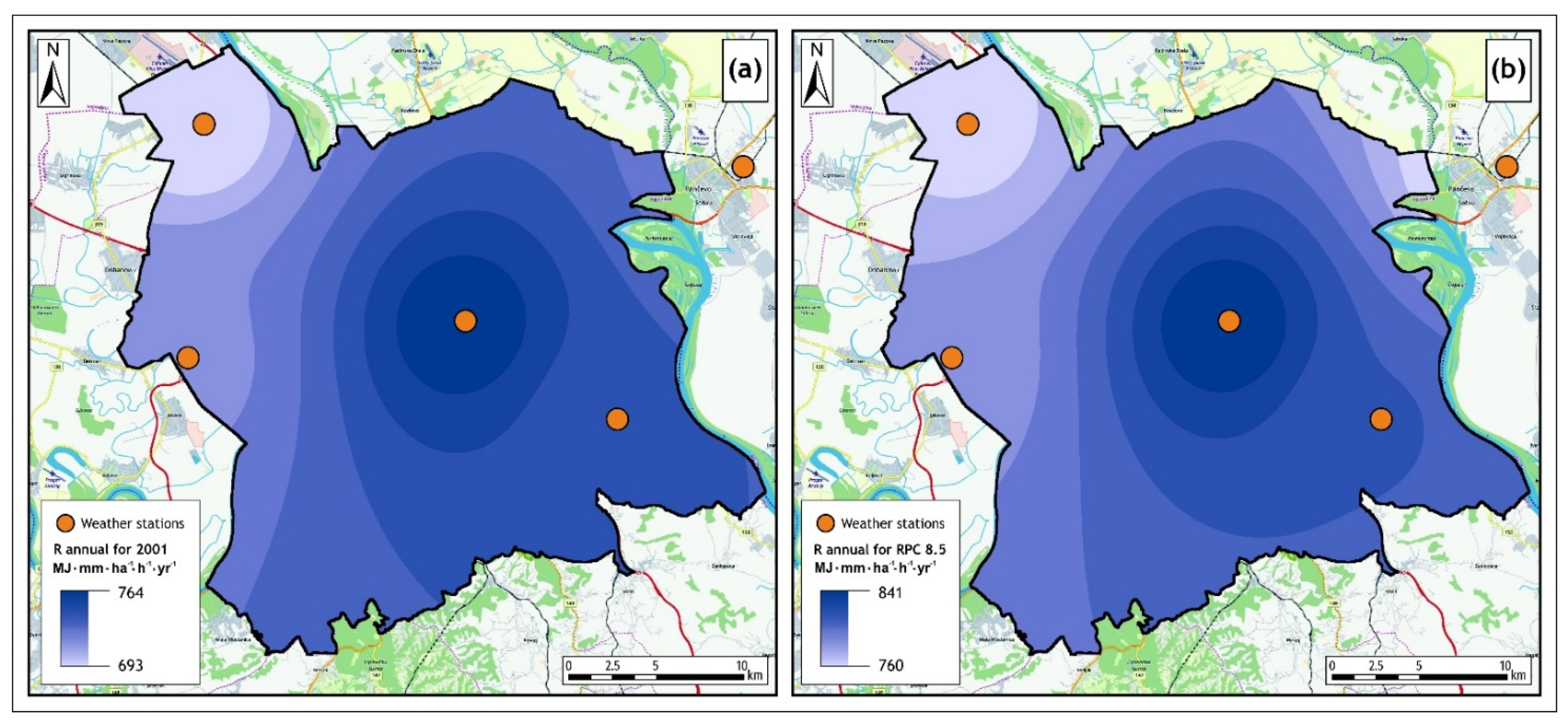
2.4.1. Rainfall Erosivity (Factor R)

Rainfall erosivity represents the potential of rain intensity to affect the erosion of a certain type of soil in a certain period [29]. The factor is a measure of the erosion intensity of rain, i.e., an index that defines the interdependence of precipitation and the production of erosion material. The annual value of factor R represents the function of EI30 which is obtained on the basis of the mathematical dependence between energy (E) and a thirty-minute rain intensity (I30) [30,59]. For the purposes of this study, due to the lack of data on thirty-minute values of precipitation, average annual precipitation amounts were used by applying a mathematical relation [60,61]:
R = b 0 · P m
R—rainfall erosivity (MJ·mm·h−1·ha−1·y−1); b0—empirical coefficient (MJ·h−1); Pm—average annual precipitation (mm).
The values of the empirical coefficient range from 1.1 to 1.5 [60], and for the purposes of this paper, the adopted value of the coefficient is 1.1. This value has been successfully applied in the territory of the Republic of Serbia [62]. Factor R is presented in the form of a raster with a spatial resolution of 30 m, using the IDW (inverse distance weighting) interpolation method based on the relevant rain gauge cells that have an impact on the study area. The obtained values of the R factor before the calculation of soil loss were compared with the extrapolated European data for the Balkan Peninsula at spatial resolutions of 500 m, which are available from the European Soil Data Centre (ESDAC) of the Joint Research Centre (JRC) [63]. In addition to this database, also consulted data obtained from studies by Bezak et al. [64], who used the Rainfall Erosivity Database at European Scale (REDES) and Uncertainties in Ensembles of Regional Reanalyses (UERRA) rainfall data for the period of 1961–2018 with a spatial resolution of 1000 m. Based on the obtained data, the results of the R factor are consistent values with small deviations.. Compared to the European data for the Balkan Peninsula the R factor in the MPB territory was reduced by 9%. Compared to the REDES database, the value of the R factor in the study area was reduced by 12%.

2.4.2. Vegetation Retention (Factor V)

Vegetation retention factor (V) has similar characteristics to factor C in the RUSLE model. Factor V, by definition, represents the degree to which the presence of vegetation and its density are expected, as well as the way in which the soil is managed to protect it from erosion [29,65]. Unlike factor C, which is obtained on the basis of empirical tables or by remote sensing, factor V in the G2 model is obtained by combining both. The input parameters are a time series of vegetation indices and constant empirical parameters of land use according to the formula:
V = e ( LU · FCover )
V—vegetation retention (normalized, dimensionless); LU—empirical parameter for land use (dimensionless); FCover—fraction of vegetation cover (dimensionless).
Factor V is dimensionless and has a value from 1 to +∞. If the value is V = 1, it represents an unfavorable way of land management, i.e., the occurrence of bare land, while the values V > 1 represent a favorable way of land management, from the aspect of reducing erosion processes. Empirical parameter LU was created based on the interpretation of empirical data sets from the Erosion Potential Method [31] and the coefficient of watershed management X·a. Parameter LU has a value from 1, for soil that is bare and subject to erosion processes, to 10, for soils that are protected from natural erosion processes. The values of the empirical parameter of land use were assigned to the land cover obtained by the method of remote detection according to the values developed by Karydas and Panagos [32]. Fractional vegetation cover (FCover) represents a vegetation bio-geophysical parameter with normalized values from 0 to 1 (completely bare to dense vegetation). Fractional vegetation cover was obtained by applying the spectral vegetation index NDVI according to the formula [66,67]:
FCover = NDVI NDVI soil NDVI veg NDVI soil
NDVI—normalized difference vegetation index; NDVI veg—value representing vegetation in the vegetation index layer; NDVI soil—the value that represents bare land in the vegetation index layer
The NDVI spectral indices were obtained for two time periods, and a set of 12 images for each month in 2001 and 2019 was used to obtain average values. In 2001, satellite images of the Landsat 5 and Landsat 7 missions were used, while satellite images of the Landsat 7 and Landsat 8 missions were used in 2019.

2.4.3. Soil Erodibility (Factor S)

The ability of soil to resist erosion agents by the sum of its properties is defined by the soil erodibility factor [29]. The formula for the RUSLE model was applied to calculate soil erodibility [29,30]:
S = { [ 2.1 · 10 4 · M 1.14 · ( 12 O M ) + 3.25   · ( s 2 ) + 2.5 · ( p 3 ) ] / 100 } · 0.1317
where S—soil erodibility (t·ha·h·ha−1·MJ−1·mm−1); M—textural factor defined as percentage of silt plus very fine sand fraction content (0.002–0.1 mm) multiplied by the factor: 100—clay fraction; OM—organic matter content in percent (%); s—soil structure class (s = 1: very fine granular, s = 2: fine granular, s = 3: medium or coarse granular, s = 4: blocky, platy or massive); and p—permeability class (p = 1: very rapid,…, p = 6: very slow); 0.1317—coefficient for converting the final value into the value of the SI unit. Class permeability is determined based on soil textural classes and tables according to Renard et al. [30].

2.4.4. Terrain Influence (Factor T)

Terrain influence factor T is a derivative of the digital terrain model and is equivalent to the terrain factor LS in the RUSLE model. Karydas and Panagos [65] suggest an equation developed by Moore and Burch [68] for the calculation of the LS terrain factor, i.e., factor T in the G2 model according to the formula:
T = ( As 22.13 ) 0.4 ·   ( sin β 0.0896 ) 1.3
where T—terrain influence (dimensionless, ≥0); As—unit contributing area (or flow accumulation), defined as the surface upstream flowing into a specific unit surface (dimensionless, >0); and β—slope gradient at the unit surface (rad).

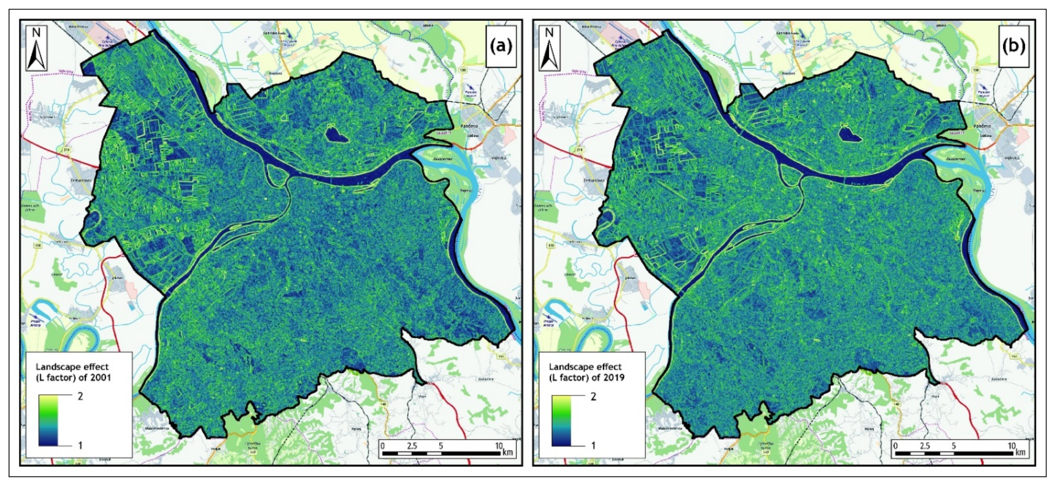
2.4.5. Landscape Effect (L)

Landscape effect (L) has the role of quantifying the influence of natural and semi-natural linear landscape elements (corridors) based on the movement of surface runoff and the development of erosion processes. Landscape ecological analyses emphasize the importance of applying edge metrics at the level of integral landscapes as indicators of landscape processes and functions to which soil erosion also belongs [69]. On the other hand, factor L can be interpreted as part of anthropogenic activities and can be compared with the factor of conservation measures P in the RUSLE methodology. The retention coefficient of sediment in the basin (Ru) in the Erosion Potential Method is based on similar motives [31] According to this method, a part of the eroded material does not reach the lowest level of the watershed, but remains in bays and depressions due to linear landscape elements (natural or introduced) that prevent its migration. To quantify this parameter, an algorithm is used for edge detection in the landscape structure, i.e., the Sobel filter, which is applied to the spectral channel from the near-infrared (NIR) part of the spectrum according to the formula [65]:
L = 1 + S f 255
Sf—Sobel filter applied to the NIR spectral channel; DNmax—maximum value of digital number on the spectral channel.
The values of the Sobel filter applied to the NIR spectral channel can have values from 0 to the maximum value of the digital number (DNmax). Digital number (DN) represents a pixel value that ranges from 0 to 255 in the case of an 8-bit record. The spatial distribution of digital numbers defines the image and the image area. The values of the landscape effect range from 1 to 2 [65].

3. Results

3.1. Land Cover Accuracy Assessment and Change Analysis

The land cover maps over the study area for the epochs of 2001 and 2019 were produced at a 30-m spatial resolution using Landsat satellite data and the RF method. The produced maps differentiate six land cover classes: water, artificial surfaces, forest, shrubs, grassland, and agriculture. All available Landsat channels were used in the classification model. The usefulness of the spectral indices in the land cover classification process were proved by several studies [70,71]; therefore, an additional set of spectral indices was included in the classification as well. These include Normalized Difference Vegetation Index (NDVI) [72], Enhanced Vegetation Index (EVI) [73] and from a group of water spectral indices proposed by Xu [74] the Modified Normalized Difference Water Index (MNDWI).
The training polygons for each LC class were created by manual vectorization, separately, for each epoch. The additional independent set of polygons was also vectorized for validation purposes. The validation polygons are created for each epoch so that they are equally distributed over the study area (Figure 2). Table 1 shows the basic information for the created training and validation datasets.
RF models were trained and applied to the study area separately for the 2001 and 2019 epochs (Figure 3). Accuracy assessment is a key component of any properly conducted remote sensing study [75,76,77,78]. Visual inspection of the produced LC maps showed meaningful distributions of the classes over the study area, which was additionally confirmed through statistical analyses. This was done by comparing outputs maps with the vectorized validation polygons, pixel-wise, and producing confusion matrixes [70,79,80]. The overall accuracy (OA), producer’s accuracy (PA), user’s accuracy (UA) and kappa coefficient of agreement (Kappa) metrics were calculated and analyzed as well as these are commonly used metrics for evaluation of land cover classification results [77,80,81].
The results shown in Table 2 show an accuracy assessment for the 2001 land cover classification. User’s accuracy for each category separately ranges from 70.39% (grasslands) to 99.82% (water bodies). Analyzing the production accuracy for each category separately, the values range from 76.65% (grasslands) to 100% (water bodies). The overall accuracy for all categories in the analyzed image is 94.52%, while the Kappa is 0.92. An assessment of the accuracy of the classification of the image from 2019 is shown in Table 3. According to the given table and confusion matrix, the user’s accuracy shows the lowest values for the grassland category (71.26%), while the highest values were recorded for water bodies (99.82%). The producer’s accuracy according to each category ranges from 66.67% (artificial surfaces) to 100% (water bodies). The overall accuracy according to all categories is 96.91%, while the Kappa is 0.95. When Kappa statistics were analyzed for both periods, the classified data agreed perfectly with the representative samples.
The created land cover maps were used to calculate the areas under change. In Table 4, the changes of each category of land cover for the observed period are shown. The biggest negative changes, i.e., loss of land, were recorded under agricultural land and grasslands. Positive changes in the areas were recorded under the category of urbanized (i.e., artificial and non-porous surfaces) and under the category of shrub vegetation. By analyzing the change matrix, for the observed period, agricultural areas had a loss of 18.66%, which was followed by changes in artificial areas, grasslands and shrub vegetation. Constant population growth has increased the demand for housing, which has put great pressure on agricultural land, but also on “arable and uncultivated land” in peripheral urban areas [11,15].

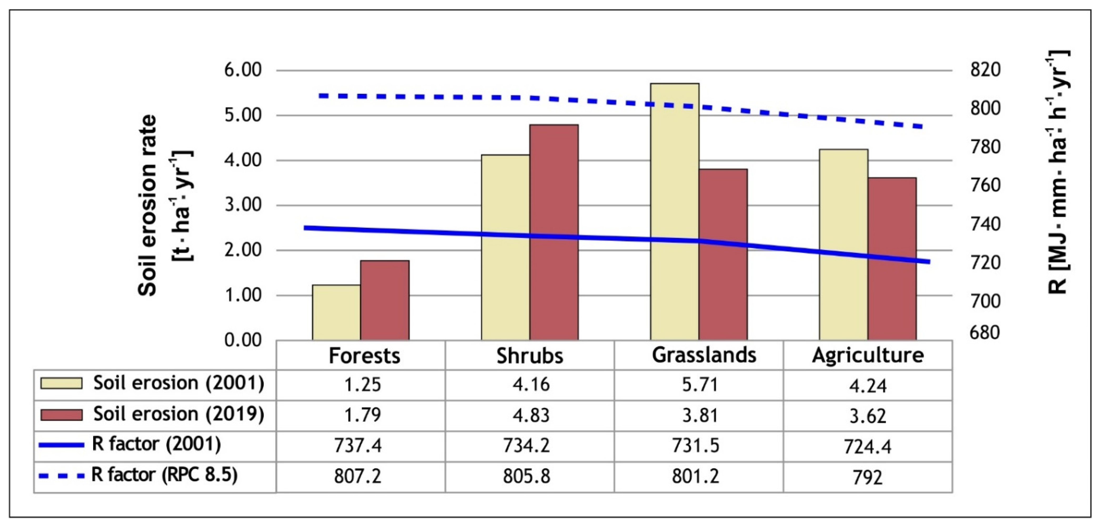
3.2. G2 Model Results

In order to deal with different representations and spatial resolutions of the used input data, first the conversion to 30-m spatial resolution rasters of some datasets was necessary. The 30-m spatial resolution is chosen to match the spatial resolution of the Landsat images and corresponding LC maps. Table 5 lists the overview of all preprocessing procedures performed on input data and corresponding G2 model inputs calculated using them.
The spatial distribution of climatic characteristics over the study area was obtained by applying the Inverse Distance Weighted (IDW) interpolation method. The IDW method is chosen because it is fast, simple and commonly used for interpolation of climate variables [82,83,84]. The EU-DEM used to describe physical–geographical characteristics also had to be resampled to a 30-m spatial resolution. This was done using the bilinear resampling technique. The last input dataset which required preprocessing is pedological map, available in scale 1:20,000. The vectorized pedology polygons were rasterized, where the output raster is also in 30-m spatial resolution. For detailed determination of the value of factor S, the IDW method was applied to soil samples. It can be considered that polygons can be converted to such spatial resolutions because various sources of errors present in the map (error of primary data acquisition, scanning and georeferencing errors, etc.) do not exceed output spatial resolution. After the input data have been successfully preprocessed, the inputs of G2 model are calculated using the previously described methodology. The results for both time periods were defined and analyzed in the following paragraphs.
The spatial distribution of factor R is shown in a raster form with a spatial resolution of 30 m. The average value of factor R is 731.19 MJ·mm·h−1·ha−1·y−1, and a value range from 693.99 to 764,907 MJ·mm·h−1·ha−1·y−1 recorded in the central part of the MPB for the first period (Figure 4a).
By simulating the parameters according to climate scenario RCP 8.5 for the middle of the century and the available mean annual precipitation, rainfall erosivity was calculated for the second period (climate-based scenario). The values of rainfall erosivity in the study area also increased from 5% to 10%. The spatial distribution of rainfall erosivity has a range of values from 760.084 up to 841,398 MJ·mm·h−1·ha−1·y−1, with an average value of 801.43 MJ·mm·h−1·ha−1·y−1 (Figure 4b).
Vegetation retention (Factor V) represents the result of remote detection in satellite images of different spatial and temporal resolutions, using a combination of spectral channels. In order to obtain data that is as relevant as possible, a set of 12 satellite images was used, one image for each month, in order to obtain average annual values. Satellite images from the vegetation and non-vegetation periods were used. For each month, one satellite image was selected which had the lowest percentage of cloudiness. Satellite images of Landsat Mission 5 and 7 were used for 2001, while satellite images of Landsat Mission 8 were used for 2019. Factor V values are dimensionless and can range from 1 to + ∞. Based on the analysis of 2001, the value of coefficient V ranged from 1 to 3079.34 with an average value of 32.83 (Figure 5a). The range of obtained values for 2019 is from 1 to 3547.43 with an average value of 39.76 (Figure 5b).
The average value of factor S is 0.041 t·ha·h·ha−1·MJ−1·mm−1 which classifies these soils in the group of highly erodible soils [29]. The values of factor S range from 0.033 up to 0.07 t·ha·h·ha−1·MJ−1·mm−1 for the investigated area in which water bodies, lakes and urbanized areas were not taken into account (Figure 6a). The obtained values of coefficient S were used for both time periods.
Terrain influence factor T was used for both time periods and is shown in Figure 6b. The range of terrain influence values ranges from 0.01 to 45.5 with an average value of 1.34. The landscape effect (L) has a range of values from 1 to 2 for both periods. The average value of factor L for 2001 for the entire study area is 1.22 (Figure 7a), while for 2019 the average value is 1.29 (Figure 7b).
The defined parameters (R, V, S, T, L) are the starting point for the calculation of soil loss according to the G2 model. Potential soil losses for both time periods are shown in the form of a raster databases with a spatial resolution of 30 m. The raster database represents the loss of soil for each pixel per unit t·ha−1·y−1. Figure 8a shows the spatial distribution of soil loss for 2001. The average value in the investigated area is 4.11 t·ha−1·y−1, and the value range is from 0 to 200.86 t·ha−1·y−1. Soil loss assessment was done only in areas that are subject to intense erosion processes. Soil losses were estimated using the G2 model based on the current land cover from 2019, according to the adopted scenario RCP 8.5 for the period of the near future and the simulation of climate parameters. The average value for the investigated area is 3.63 t·ha−1·y−1, and the values range from 0 to 193.11 t·ha−1·y−1 (Figure 8b). In the case of both periods, the investigated area belongs to the category of medium erosion, although there was a slight decrease in the average value of soil loss of 11.68% in 2019. According to the spatial layout shown in Figure 8a,b, and according to Table 6, all forms of the category of destructiveness are present in the research area. In addition to the analysis of the shares of different areas, a comparison was performed in relation to the land cover as one of the most dynamic parameters. According to Figure 9, the average values of loss are shown in relation to areas with a high degree of porous surfaces. Water bodies and urbanized artificial surfaces with a high degree of non-porous surfaces are excluded from the analysis of soil loss and comparison.

4. Discussion

The intense expansion of urban functions and the need for new space for the growth of cities leads to changes in the structure of land cover, i.e., to the transformation of agricultural, as well as natural and semi-natural elements, into non-porous areas. Such surfaces cause the cessation of natural processes and have a highly negative impact on the land surface and groundwater regime causing the intensification of rapid surface runoff, the frequency of high waters, urban floods, and the intensification of erosion processes [85]. These changes lead to an increased risk for the infrastructure (road network and bridges), residential and commercial zones, sewerage and drainage systems, water supply sources and reservoirs, thus disrupts vital urban functions [11,86,87]. On the other hand, soil erosion can presents a vector of negative impacts and lead to endangered public health through sources pollution affecting water supply [88], the loss of fertility of agricultural land by nutrient removal [89,90], as well as to participate in factors that cause climate change, given that eroded areas have increased carbon emissions into the atmosphere [91]
Based on these facts, there is an increased need for the research of modalities for determining relevant research procedures, methods and techniques that will indicate the spatial and temporal scale of the occurrence and development of erosion processes and the environmental degradation forms. Contemporary cities are a dynamic conglomeration of urban functions that primarily depend on the built infrastructure and facilities, but the quality and safety of life of city dwellers also depends on the stability of natural and semi-natural elements as well as on the productivity of agricultural land. The functionality and safety of life of the inhabitants is related to the quality of the environment, so urban landscapes can be interpreted as an outdoor laboratory that has the potential to contribute to determining the modalities of the degradation processes monitoring.
Soil loss estimation using the G2 model was analyzed for two time periods, i.e., for the beginning of the entry into force of the Master Plan of Belgrade (2001) and for the period that is close to the end of its validity (2019). For the first period, the annual soil loss ranged from 0 to 200.86 t·ha−1·y−1, with an average value 4.11 t·ha−1·y−1. The analysis of the second period revealed an annual soil loss of which values range from 0 to 193.11 t·ha−1·y−1, with an average value of 3.63 t·ha−1·y−1. Comparative analysis identified a slight reduction in soil losses. The total area endangered by soil erosion was reduced from 526.46 to 481.39 km2, which is a decrease of 8.56%. Despite this, all seven categories are present for both observed periods. In other words, the change is not so pronounced that there is a disappearance of a certain category of loss, but there is a distribution of quantities within categories, as well as a certain change in area categories (Table 6). The share of areas in the category of low medium erosion increased from 2.43% in 2001, to 2.95% in 2019, which represents a growth of 10.95%. In addition to this category, the areas in the category of medium erosion increased from 5.38% to 8.05%, and an increase of 36.78% was recorded for that area. In contrast, the areas of high and very high category of erosion were reduced by 30.02% and 21.92%, respectively, while the categories of high-medium erosion and very low erosion were reduced by 8.04% and 9.49%, respectively. Low-intensity erosion, which is classified in the category of low erosion, has experienced the lowest degree of modification, so that it still plays a dominant role in the dynamics of soil erosion. According to Figure 8a,b, the spatial distribution is shown by the categories of soil erosion intensity. Areas with a loss of over 1 t·ha−1·y−1 were identified for both periods in the southern areas of the area of hilly and mountainous regions with developed intermittent and permanent streams with torrential characteristics. The highest soil loss was identified on agricultural land located on steep slopes. The results of the G2 model indicate that the highest losses were recorded in places where grasslands and shrub vegetation change into agricultural areas. The categories of weak and very weak erosion with the soil loss of below 1 t·ha−1·y−1 were identified in the northern part, mainly in the plains and under agricultural areas. According to the land use defined in the MPB, these soil losses occur in planned economic, agricultural and green areas.
In relation to the spatial distribution of the category of erosion processes, soil loss was also analyzed for different land covers. Land use change as part of urban strategies and the consequent change in land cover are dynamic factors that change under the influence of political, social and bio-physical elements [92]. These changes were recognized as an essential group of driving forces that determine the in the quality of the environment of urban areas, of which the range of impacts reaches different spatial and temporal dimensions [93,94]. Urbanization processes mainly develop on areas that do not have a clearly defined purpose or are part of a city’s developmental strategy, such as land cover classes that belong to grasslands and partly to agricultural lands. As these classes of land cover show the largest soil losses during the analyzed period, their decrease in the average value of soil loss was recorded. A decrease of 0.63 t·ha−1·y−1 was recorded for agricultural areas, while there was a decrease of 1.90 t·ha−1·y−1 for grasslands. Considering that the current state of land cover and simulated climatic parameters according to scenario RCP 8.5 were applied for the second period in the analysis (scenario of constant increase of greenhouse gas emissions), the reduction of average soil losses on agricultural areas and grasslands is justified. On the other hand, as a consequence of this process, the pressure on natural and semi-natural classes of land cover, i.e., on the remaining fragments of forest and shrub vegetation, increased. In these areas, there was an increase in the average values of soil loss according to climate scenario RCP 8.5. The average value of soil loss in forest areas increased by 0.54 t·ha−1·y−1, while in the area of shrub vegetation it increased by 0.67 t·ha−1·y−1. The obtained results indicate that in areas where urban functions are dominant natural and semi-natural elements as carriers of ecological characteristics are endangered by soil erosion processes. It is necessary to change the attitude towards these areas in urban plans, considering the fact that they represent a vital component of the urban landscape.

5. Conclusions

Soil erosion is a global environmental problem that negatively affects ecosystem services, safety and the economy of urban landscapes. Urbanization processes, as a consequence of the need for new spaces and solving of the population growth problem, cause the acceleration of natural soil erosion processes, which are becoming a serious problem for modern cities in light of climate change. Soil erosion modeling using authoritative and detailed databases, such as the G2 model applied with remote sensing methods, enable the precise identification of soil erosion intensity categories and the use of a climate model adds a dimension of reality to their prediction.
The results obtained by applying the G2 model indicate that the processes of urbanization cause the distribution of soil losses and sediment production in such a way that the classes of natural and semi-natural elements stand out as particularly fragile categories. The increase in porous surfaces adds additional pressure to these areas which increases the intensity of water and pluvial erosion. In addition, the classes of forest and shrub elements linearly become significant hazard zones in urbanized conditions and through an increased surface runoff and a more dynamic genesis of torrential floods, they transfer their impact to other surrounding areas. This constellation of altered environmental parameters causes other problems that degrade the quality of life in urban areas, such as the increased heat island effect, the loss of agricultural land fertility, acidification and salinization of soils, reduction of carbon content and compaction, increased greenhouse effect, etc.
The identified zones responsible for the excessive production of eroded material can be recognized as hazard zones and their spatial determination plays a significant role in the environmental risk assessment of urban landscape. The location of hazard zones and prediction of their development in the context of urbanization and climate change enables the elaboration of city development scenarios, analysis of consequences as well as configuration of a system of guidelines for imitating their further impacts. Adding a spatial context to erosion processes is the starting point for regional policies related to soil resources and soil conservation, which enables recognition of their place in spatial planning documents and city strategies. Techniques that support spatial analysis and synthesis of heterogeneous data have formed a powerful nexus (geographic information systems—modelling methods—remote sensing) to create a database of soil erosion categories that allows a realistic assessment of the ecological stability in urban areas.

Author Contributions

Conceptualization, S.P. and B.R.; data curation, V.M.; formal analysis, N.Ž.; resources, N.Ž.; methodology, S.P. and B.R.; validation: J.K.; software: S.P. and J.K.; supervision, R.R. and B.R.; visualization, S.P.; writing—original draft, S.P.; writing—review and editing, S.P., B.R., R.R., J.K., V.M. and N.Ž. All authors have read and agreed to the published version of the manuscript.

Funding

We would like to thank the Serbian Ministry of Education, Science and Technological Development, grant number 451-03-9/2021-14/200169, for financing scientific research at the Faculty of Forestry University of Belgrade in 2021.

Institutional Review Board Statement

Not applicable.

Informed Consent Statement

Not applicable.

Data Availability Statement

Data is contained within the article.

Conflicts of Interest

The authors declare no conflict of interest.

References

  1. Jain, M.K.; Das, D. Estimation of sediment yield and areas of soil erosion and deposition for watershed prioritization using GIS and remote sensing. Water Resour. Manag. 2010, 24, 2091–2112. [Google Scholar] [CrossRef]
  2. Milliman, J.D.; Syvitski, J.P. Geomorphic/tectonic control of sediment discharge to the ocean: The importance of small mountainous rivers. J. Geol. 1992, 100, 525–544. [Google Scholar] [CrossRef]
  3. Zhang, X.; Cao, W.; Guo, Q.; Wu, S. Effects of landuse change on surface runoff and sediment yield at different watershed scales on the Loess Plateau. Int. J. Sediment Res. 2010, 25, 283–293. [Google Scholar] [CrossRef]
  4. Zhu, C.; Li, Y. Long-Term Hydrological Impacts of Land Use/Land Cover Change from 1984 to 2010 in the Little River Watershed, Tennessee. Int. Soil Water Conserv. Res. 2014, 2, 11–21. [Google Scholar] [CrossRef] [Green Version]
  5. Bennett, H.H. Elements of Soil Conservation; McGraw-Hill Book Company, Inc.: New York, NY, USA, 1947; 406p. [Google Scholar] [CrossRef]
  6. Ahmadi, H. Applied Geomorphology (Water Erosion)-Google Scholar. Available online: https://scholar.google.com/scholar?hl=fr&as_sdt=0,5&cluster=9947268861899941313 (accessed on 18 April 2021).
  7. Zhang, W.; Zhou, J.; Feng, G.; Weindorf, D.C.; Hu, G.; Sheng, J. Characteristics of water erosion and conservation practice in arid regions of Central Asia: Xinjiang Province, China as an example. Int. Soil Water Conserv. Res. 2015, 3, 97–111. [Google Scholar] [CrossRef] [Green Version]
  8. Lal, R. Soil degradation by erosion. Land Degrad. Dev. 2001, 12, 519–539. [Google Scholar] [CrossRef]
  9. Pimentel, D.; Kounang, N. Ecology of soil erosion in ecosystems. Ecosystems 1998, 1, 416–426. [Google Scholar] [CrossRef]
  10. Pimentel, D. Soil erosion: A food and environmental threat. Environ. Dev. Sustain. 2006, 8, 119–137. [Google Scholar] [CrossRef]
  11. Shikangalah, R.N.; Jeltsch, F.; Blaum, N.; Mueller, E.N. A review on urban soil water erosion. J. Stud. Humanit. Soc. Sci. 2016, 5, 163–178. [Google Scholar]
  12. Radić, B.; Gavrilović, S. Natural Habitat Loss: Causes and Implications of Structural and Functional Changes; Springer: Cham, Switzerland, 2020; pp. 1–14. Available online: https://link.springer.com/referenceworkentry/10.1007/978-3-319-71065-5_6-1 (accessed on 2 April 2020).
  13. Kundzewicz, Z. Flood risk and vulnerability in the changing climate. Ann. Wars. Univ. Life Sci. SGGW Land Reclam. 2008, 39, 21–31. [Google Scholar] [CrossRef]
  14. Kusky, M.T. Encyclopedia of Earth and Space Science; Science Encyclopedia; Katherine, E.C., Ed.; Facts on File: New York, NY, USA, 2020; ISBN 9780816070053. Available online: https://www.amazon.com/Encyclopedia-Earth-Space-Science-Set/dp/0816070059 (accessed on 24 March 2021).
  15. Pribadi, D.O.; Vollmer, D.; Pauleit, S. Impact of peri-urban agriculture on runoff and soil erosion in the rapidly developing metropolitan area of Jakarta, Indonesia. Reg. Environ. Chang. 2018, 18, 2129–2143. [Google Scholar] [CrossRef]
  16. Szendreine-Koren, E.; Nemeskeri, I. Water Management of forest soils below different soil types. Carpathian J. Earth Environ. Sci. 2007, 2, 17–24. [Google Scholar]
  17. Ristić, R.; Kostadinov, S.; Abolmasov, B.; Dragićević, S.; Trivan, G.; Radić, B.; Trifunović, M.; Radosavljević, Z. Torrential floods and town and country planning in Serbia. Nat. Hazards Earth Syst. Sci. 2012, 12, 23–35. [Google Scholar] [CrossRef]
  18. Herslund, L.B.; Jalayer, F.; Jean-Baptiste, N.; Jørgensen, G.; Kabisch, S.; Kombe, W.; Lindley, S.; Nyed, P.K.; Pauleit, S.; Printz, A.; et al. A multi-dimensional assessment of urban vulnerability to climate change in Sub-Saharan Africa. Nat. Hazards 2016, 82, 149–172. [Google Scholar] [CrossRef]
  19. de Vente, J.; Poesen, J. Predicting soil erosion and sediment yield at the basin scale: Scale issues and semi-quantitative models. Earth Sci. Rev. 2005, 71, 95–125. [Google Scholar] [CrossRef]
  20. Foster, G.R. Advances in wind and water erosion prediction. J. Soil Water Conserv. 1991, 46, 27–29. [Google Scholar]
  21. Laflen, J.M.; Lane, L.J.; Foster, G. WEPP: A new generation of erosion prediction technology. J. Soil Water Conserv. 1991, 46, 34–38. [Google Scholar]
  22. Boardman, J. Soil erosion science: Reflections on the limitations of current approaches. Catena 2006, 68, 73–86. [Google Scholar] [CrossRef]
  23. Renschler, C.S.; Harbor, J. Soil erosion assessment tools from point to regional scales—The role of geomorphologists in land management research and implementation. Geomorphology 2002, 47, 189–209. [Google Scholar] [CrossRef]
  24. Renschler, C.S. Designing geo-spatial interfaces to scale process models: The GeoWEPP approach. Hydrol. Process. 2003, 17, 1005–1017. [Google Scholar] [CrossRef]
  25. Wu, J.; Li, H. Concepts of scale and scaling. In Scaling and Uncertainty Analysis in Ecology: Methods and Applications; Springer: Dodlerk, The Netherlands, 2006; pp. 3–15. ISBN 1402046642. Available online: http://www.informationweek.com/news/201202317 (accessed on 2 April 2020).
  26. Mitasova, H.; Barton, M.; Ullah, I.; Hofierka, J.; Harmon, R.S. GIS-Based Soil Erosion Modeling. In Treatise on Geomorphology; Elsevier Inc.: Amsterdam, The Netherlands, 2013; Volume 3, pp. 228–258. ISBN 9780080885223. Available online: https://www.sciencedirect.com/science/article/pii/B978012374739600052X (accessed on 2 April 2020).
  27. Panagos, P.; Karydas, C.G.; Gitas, I.Z.; Montanarella, L. Monthly soil erosion monitoring based on remotely sensed biophysical parameters: A case study in Strymonas river basin towards a functional pan-European service. Int. J. Digit. Earth 2012, 5, 461–487. [Google Scholar] [CrossRef]
  28. Panagos, P.; Christos, K.; Cristiano, B.; Ioannis, G. Seasonal monitoring of soil erosion at regional scale: An application of the G2 model in crete focusing on agricultural land uses. Int. J. Appl. Earth Obs. Geoinf. 2014, 27, 147–155. [Google Scholar] [CrossRef]
  29. Wischmeier, W.H.; Smith, D.D. Predicting Rainfall Erosion Losses—A Guide to Conservation Planning; United States Department of Agriculture: Washington, DC, USA, 1978. Available online: https://naldc.nal.usda.gov/download/CAT79706928/PDF (accessed on 5 March 2021).
  30. Renard, K.; Foster, G.; Weesies, G.; McCool, D.; Yoder, D. Predicting soil erosion by water: A guide to conservation planning with the Revised Universal Soil Loss Equation (RUSLE). In Agriculture Handbook No. 703; United States Department of Agriculture: Washington, DC, USA, 1997. Available online: https://www.ars.usda.gov/ARSUserFiles/64080530/RUSLE/AH_703.pdf (accessed on 12 March 2021).
  31. Gavrilović, S. Engineering of Torrents and Erosion; Journal of Construction (Special Issue): Belgrade, Yugoslavia, 1972. (In Serbia) [Google Scholar]
  32. Karydas, C.G.; Zdruli, P.; Koci, S.; Sallaku, F. Monthly Time-Step Erosion Risk Monitoring of Ishmi-Erzeni Watershed, Albania, Using the G2 Model. Environ. Model. Assess. 2015, 20, 657–672. [Google Scholar] [CrossRef]
  33. Zdruli, P.; Karydas, C.G.; Dedaj, K.; Salillari, I.; Cela, F.; Lushaj, S.; Panagos, P. High resolution spatiotemporal analysis of erosion risk per land cover category in Korçe region, Albania. Earth Sci. Inform. 2016, 9, 481–495. [Google Scholar] [CrossRef]
  34. Karydas, C.G.; Panagos, P. Modelling monthly soil losses and sediment yields in Cyprus. Int. J. Digit. Earth 2016, 9, 766–787. [Google Scholar] [CrossRef]
  35. Artun, O.; Dinc, A.O.; Satir, O. Estimation of soil losses using various soil erosion models in a sample plot in Mediterranean part of Turkey. Fresenius Environ. Bull. 2017, 26, 3385–3394. [Google Scholar]
  36. Halecki, W.; Kruk, E.; Ryczek, M. Evaluation of water erosion at a mountain catchment in Poland using the G2 model. Catena 2018, 164, 116–124. [Google Scholar] [CrossRef]
  37. Karydas, C.; Bouarour, O.; Zdruli, P. Mapping Spatio-Temporal Soil Erosion Patterns in the Candelaro River Basin, Italy, Using the G2 Model with Sentinel2 Imagery. Geosciences 2020, 10, 89. [Google Scholar] [CrossRef] [Green Version]
  38. Antonović, G.; Živanović, Ž.; Bogdanović, M.; Ćorović, R.; Trifunović, M. Soils of South-Eastern Srem; City Geodetic Authority: Belgrade, Yugoslavia, 1976.
  39. Antonović, G.; Živanović, Ž.; Bogdanović, M.; Ćorović, R.; Trifunović, M. Soils in the Area of Belgrade South of the Sava and Danube; City Geodetic Authority: Belgrade, Yugoslavia, 1976.
  40. Đurđević, V.; Vuković, A.; Vujadinović-Mandić, M. Climate Changes Observed in Serbia and Future Climate Projections Based on Different Scenarios of Future Emissions. Available online: https://www.google.com/url?sa=t&rct=j&q=&esrc=s&source=web&cd=&ved=2ahUKEwjp5_iY7cHvAhXI26QKHc0_AKoQFjAAegQIB-BAD&url=http%3A%2F%2Fwww.klimatskepromene.rs%2Fwp-content%2Fuploads%2F2019%2F11%2FCLIMATE-CHANGES-OBSERVED-IN-SERBIA-AND-FUTURE-CLIMATE-PROJECTIO (accessed on 15 February 2021).
  41. Ristić, R.; Radić, B.; Miljanović, V.; Trivan, G.; Ljujić, M.; Letić, L.; Savić, R. Blue-green corridors as a tool for mitigation of natural hazards and restoration of urbanized areas: A case study of belgrade city. Spatium 2013, 504, 18–22. [Google Scholar] [CrossRef]
  42. Ristić, R.; Radić, B.; Trivan, G.; Malusevic, I. “Blue-green” corridors as a tool for erosion and stream control in highly urbanized areas—Case study of Belgrade city. IAHS-AISH Proc. Rep. 2014, 363, 315–320. [Google Scholar]
  43. Souverijns, N.; Buchhorn, M.; Horion, S.; Fensholt, R.; Verbeeck, H.; Verbesselt, J.; Herold, M.; Tsendbazar, N.E.; Bernardino, P.N.; Somers, B.; et al. Thirty Years of Land Cover and Fraction Cover Changes over the Sudano-Sahel Using Landsat Time Series. Remote Sens. 2020, 12, 3817. [Google Scholar] [CrossRef]
  44. Phiri, D.; Morgenroth, J. Review Developments in Landsat Land Cover Classification Methods: A Review. Remote Sens. 2017, 9, 967. [Google Scholar] [CrossRef] [Green Version]
  45. Hansen, M.C.; Loveland, T.R. A review of large area monitoring of land cover change using Landsat data. Remote Sens. Environ. 2012, 122, 66–74. [Google Scholar] [CrossRef]
  46. Afrin, S.; Gupta, A.; Farjad, B.; Ahmed, M.R.; Achari, G.; Hassan, Q.K. Development of Land-Use/Land-Cover Maps Using Landsat-8 and MODIS Data, and Their Integration for Hydro-Ecological Applications. Sensors 2019, 19, 4891. [Google Scholar] [CrossRef] [PubMed] [Green Version]
  47. Alam, A.; Bhat, M.S.; Maheen, M. Using Landsat satellite data for assessing the land use and land cover change in Kashmir valley. GeoJournal 2019, 85, 1529–1543. [Google Scholar] [CrossRef] [Green Version]
  48. Fassnacht, F.E.; Schiller, C.; Kattenborn, T.; Zhao, X.; Qu, J. A Landsat-based vegetation trend product of the Tibetan Plateau for the time-period 1990–2018. Sci. Data 2019, 6, 1–11. [Google Scholar] [CrossRef]
  49. Cai, Y.; Liu, S.; Lin, H. Monitoring the Vegetation Dynamics in the Dongting Lake Wetland from 2000 to 2019 Using the BEAST Algorithm Based on Dense Landsat Time Series. Appl. Sci. 2020, 10, 4209. [Google Scholar] [CrossRef]
  50. Lin, L.; Hao, Z.; Post, C.J.; Mikhailova, E.A.; Yu, K.; Yang, L.; Liu, J. Monitoring land cover change on a rapidly urbanizing island using google earth engine. Appl. Sci. 2020, 10, 7336. [Google Scholar] [CrossRef]
  51. Schultz, M.; Clevers, J.G.; Carter, S.; Verbesselt, J.; Avitabile, V.; Quang, H.V.; Herold, M. Performance of vegetation indices from Landsat time series in deforestation monitoring. Int. J. Appl. Earth Obs. Geoinf. 2016, 52, 318–327. [Google Scholar] [CrossRef]
  52. Wagle, N.; Acharya, T.D.; Kolluru, V.; Huang, H.; Lee, D.H. Multi-temporal land cover change mapping using google earth engine and ensemble learning methods. Appl. Sci. 2020, 10, 8083. [Google Scholar] [CrossRef]
  53. Carreño-Conde, F.; Sipols, A.E.; Simón, C.; Mostaza-Colado, D. A forecast model applied to monitor crops dynamics using vegetation indices (Ndvi). Appl. Sci. 2021, 11, 1859. [Google Scholar] [CrossRef]
  54. Wiesmeier, M.; Barthold, F.; Blank, B.; Kögel-Knabner, I. Digital mapping of soil organic matter stocks using Random Forest modeling in a semi-arid steppe ecosystem. Plant Soil 2011, 340, 7–24. [Google Scholar] [CrossRef]
  55. Ballabio, C.; Jiskra, M.; Osterwalder, S.; Borrelli, P.; Montanarella, L.; Panagos, P. A spatial assessment of mercury content in the European Union topsoil. Sci. Total Environ. 2021, 769, 144755. [Google Scholar] [CrossRef] [PubMed]
  56. Breiman, L. Random forests. Mach. Learn. 2001, 45, 5–32. [Google Scholar] [CrossRef] [Green Version]
  57. Louis, J.; Debaecker, V.; Pflug, B.; Main-Knorn, M.; Bieniarz, J.; Mueller-Wilm, U.; Cadau, E.; Gascon, F. Sentinel-2 SEN2COR: L2A processor for users. Eur. Sp. Agency 2016, SP-740, 9–13. [Google Scholar]
  58. Thanh Noi, P.; Kappas, M. Comparison of Random Forest, k-Nearest Neighbor, and Support Vector Machine Classifiers for Land Cover Classification Using Sentinel-2 Imagery. Sensors 2017, 18, 18. [Google Scholar] [CrossRef] [Green Version]
  59. Morgan, R.P. Soil Erosion and Conservation, 3rd ed.; National Soil Resources Institute, Cranfield University: Bedford, UK, 2005; Available online: https://www.wiley.com/en-us/Soil+Erosion+and+Conservation%2C+3rd+Edition-p-9781405117814 (accessed on 15 February 2021).
  60. Van der Knijff, J.M.; Jones, R.J.; Montanarella, L. Assessment in Italy Soil Erosion Risk. EUR 19044 EN; The Official Publications Office of the European Communities: Luxembourg, 2000. [Google Scholar]
  61. Grimm, M.; Jones, R.J.; Rusco, E.; Montanarella, L. Soil erosion risk in Italy: A revised USLE approach. Eur. Soil Bur. Res. Rep. 2003, 11, 23. [Google Scholar]
  62. Perović, V.; Kadović, R.; Djurdjević, V.; Braunović, S.; Čakmak, D.; Mitrović, M.; Pavlović, P. Effects of changes in climate and land use on soil erosion: A case study of the Vranjska Valley, Serbia. Reg. Environ. Chang. 2019, 19, 1035–1046. [Google Scholar] [CrossRef]
  63. Panagos, P.; Ballabio, C.; Borrelli, P.; Meusburger, K.; Klik, A.; Rousseva, S.; Tadić, M.P.; Michaelides, S.; Hrabalíková, M.; Olsen, P.; et al. Rainfall erosivity in Europe. Sci. Total Environ. 2015, 511, 801–814. [Google Scholar] [CrossRef] [Green Version]
  64. Bezak, N.; Ballabio, C.; Mikoš, M.; Petan, S.; Borrelli, P.; Panagos, P. Reconstruction of past rainfall erosivity and trend detection based on the REDES database and reanalysis rainfall. J. Hydrol. 2020, 590, 125372. [Google Scholar] [CrossRef]
  65. Karydas, C.G.; Panagos, P. The G2 erosion model: An algorithm for month-time step assessments. Environ. Res. 2018, 161, 256–267. [Google Scholar] [CrossRef]
  66. Carlson, T.N.; Ripley, D.A. On the relation between NDVI, fractional vegetation cover, and leaf area index. Remote Sens. Environ. 1997, 62, 241–252. [Google Scholar] [CrossRef]
  67. Gutman, G.; Ignatov, A. The derivation of the green vegetation fraction from NOAA/AVHRR data for use in numerical weather prediction models. Int. J. Remote Sens. 1998, 19, 1533–1543. [Google Scholar] [CrossRef]
  68. Moore, I.D.; Burch, G.J. Physical Basis of the Length-slope Factor in the Universal Soil Loss Equation. Soil Sci. Soc. Am. J. 1986, 50, 1294–1298. [Google Scholar] [CrossRef]
  69. Radić, B. Erosion as Factor of Landscape Degradation in Serbian Ski-Resorts. Ph.D. Thesis, Faculty of Forestry, University of Belgrade, Belgrade, Serbia, 2014. [Google Scholar]
  70. Abdi, A.M. Land cover and land use classification performance of machine learning algorithms in a boreal landscape using Sentinel-2 data. GIScience Remote Sens. 2020, 57, 1–20. [Google Scholar] [CrossRef] [Green Version]
  71. Niculescu, S.; Talab Ou Ali, H.; Billey, A. Random forest classification using Sentinel-1 and Sentinel-2 series for vegetation monitoring in the Pays de Brest (France). In Remote Sensing for Agriculture, Ecosystems, and Hydrology XX; Neale, C.M., Maltese, A., Eds.; SPIE: Washington, DC, USA, 2018; Volume 10783, p. 6. Available online: https://spie.org/Publications/Proceedings/Paper/10.1117/12.2325546?SSO=1 (accessed on 8 March 2021).
  72. Deering, D.W. Rangeland Reflectance Characteristics Measured by Aircraft and Spacecraft Sensors; Texas A&M University Libraries: College Station, TX, USA, 1978; Available online: https://oaktrust.library.tamu.edu/handle/1969.1/DISSERTATIONS-253780 (accessed on 9 March 2021).
  73. Didan, K.; Munoz, A.B.; Solano, R.; Huete, A. MODIS Vegetation Index User’s Guide (Collection 6); University of Arizona: Tucson, AZ, USA, 2015; p. 31. Available online: https://vip.arizona.edu/documents/MODIS/MODIS_VI_UsersGuide_June_2015_C6.pdf (accessed on 12 March 2021).
  74. Xu, H. Modification of normalised difference water index (NDWI) to enhance open water features in remotely sensed imagery. Int. J. Remote Sens. 2006, 27, 3025–3033. [Google Scholar] [CrossRef]
  75. Congalton, R.G. A review of assessing the accuracy of classification of remotely sensed data. Remote Sens. Environ. 1991, 37, 35–46. [Google Scholar] [CrossRef]
  76. Goodchild, M.F.; Guoqing, S.U.; Shiren, Y. Development and test of an error model for categorical data. Int. J. Geogr. Inf. Syst. 1992, 6, 87–103. [Google Scholar] [CrossRef]
  77. Khorram, S.; van der Wiele, C.F.; Koch, F.H.; Nelson, S.A.; Potts, M.D. Data Acquisition. In Principles of Applied Remote Sensing; Springer International Publishing: Cham, Switzerland, 2016; pp. 21–67. [Google Scholar]
  78. Paine, D.P.; Kiser, J.D. Aerial Photography and Image Interpretation, 2nd ed.; John Wiley, Inc.: New York, NY, USA, 2003. [Google Scholar]
  79. Levin, N. Fundamentals of Remote Sensing; Remote Sensing Laboratory, Geography Department, Tel Aviv University: Tel Aviv, Israel, 1999. [Google Scholar]
  80. Tempfli, K.; Huurneman, G.C.; Bakker, W.H.; Janssen, L.L.; Feringa, W.F.; Gieske, A.S.; Grabmaier, K.A.; Hecker, C.A.; Horn, J.A.; Kerle, N.; et al. Principles of Remote Sensing: An Introductory Textbook; International Institute for Geo-Information Science and Earth Observation: Enschede, The Netherlands, 2009; ISBN 978-90-6164-270-1. Available online: https://research.utwente.nl/en/publications/principles-of-remote-sensing-an-introductory-textbook-4 (accessed on 12 March 2021).
  81. Olofsson, P.; Foody, G.M.; Herold, M.; Stehman, S.V.; Woodcock, C.E.; Wulder, M.A. Good practices for estimating area and assessing accuracy of land change. Remote Sens. Environ. 2014, 148, 42–57. [Google Scholar] [CrossRef]
  82. Chen, T.; Ren, L.; Yuan, F.; Yang, X.; Jiang, S.; Tang, T.; Liu, Y.; Zhao, C.; Zhang, L. Comparison of spatial interpolation schemes for rainfall data and application in hydrological modeling. Water 2017, 9, 342. [Google Scholar] [CrossRef] [Green Version]
  83. Yang, X.; Xie, X.; Liu, D.L.; Ji, F.; Wang, L. Spatial Interpolation of Daily Rainfall Data for Local Climate Impact Assessment over Greater Sydney Region. Adv. Meteorol. 2015, 2015, 563629. [Google Scholar] [CrossRef] [Green Version]
  84. Robinson, T.P.; Metternicht, G. Testing the performance of spatial interpolation techniques for mapping soil properties. Comput. Electron. Agric. 2006, 50, 97–108. [Google Scholar] [CrossRef]
  85. Scalenghe, R.; Ajmone-Marsan, F. The anthropogenic sealing of soils in urban areas. Landsc. Urban Plan. 2009, 90, 1–10. [Google Scholar] [CrossRef]
  86. Strahler, A.H. Introducing Physical Geography, 5th ed.; John Wiley & Sons: Chichester, UK, 2010. [Google Scholar]
  87. Merz, B.; Kreibich, H.; Schwarze, R.; Thieken, A. Review article “assessment of economic flood damage”. Nat. Hazards Earth Syst. Sci. 2010, 10, 1697–1724. [Google Scholar] [CrossRef]
  88. Gaffield, S.J.; Goo, R.L.; Richards, L.A.; Jackson, R.J. Public Health Effects of Inadequately Managed Stormwater Runoff. Am. J. Public Health 2003, 93, 1527–1533. [Google Scholar] [CrossRef]
  89. Poesen, J.W.; Hooke, J.M. Erosion, flooding and channel management in Mediterranean environments of southern Europe. Prog. Phys. Geogr. 1997, 21, 157–199. [Google Scholar] [CrossRef]
  90. Kheir, R.B. A conditional GIS-interpolation-based model for mapping soil-water erosion processes in Lebanon. Land Degrad. Dev. 2008, 19, 122–135. [Google Scholar] [CrossRef]
  91. Gaiser, T.; Stahr, K.; Billen, N.; Mohammad, M.A. Modeling carbon sequestration under zero tillage at the regional scale. I. The effect of soil erosion. Ecol. Model. 2008, 218, 110–120. [Google Scholar] [CrossRef]
  92. Karsidi, A. Spatial Analysis of Land Use/Land Cover Change Dynamics Using Remote Sensing and Geographic Information Systems: A Case Study in the Down Stream and Surroundings of the Ci Tarum Watershed/Asep Karsidi. 2004. Available online: https://digital.library.adelaide.edu.au/dspace/handle/2440/22077 (accessed on 11 March 2021).
  93. Turner, B.; Meyer, W.B.; Skole, D.L. Global land-use/land-cover change: Towards an integrated study. Ambio Stockh. 1994, 23, 91–95. [Google Scholar]
  94. Brovelli, M.A.; Fahl, F.C.; Minghini, M.; Molinari, M.E. Land user and land cover maps of Europe: A webgis platform. In Proceedings of the International Archives of the Photogrammetry, Remote Sensing and Spatial Information Sciences-ISPRS Archives; International Society for Photogrammetry and Remote Sensing: Christian Heipke, Germany, 2016; Volume 41, pp. 913–917. Available online: https://ui.adsabs.harvard.edu/abs/2016ISPAr41B7..913B/abstract (accessed on 12 March 2021).
Figure 1. Study area.
Applsci 11 04154 g001
Figure 2. Samples of the polygons for training and land cover validation for 2001 (a) and 2019 (b).
Applsci 11 04154 g002
Figure 3. Land cover for 2001 (a) and 2019 (b).
Applsci 11 04154 g003
Figure 4. Spatial distribution of factor R for 2001 (a) and for climate-based scenario (b).
Applsci 11 04154 g004
Figure 5. Spatial distribution of coefficient V for 2001 (a) and 2019 (b).
Applsci 11 04154 g005
Figure 6. Spatial distribution of soil erodibility coefficient S (a) and terrain influence factor T (b).
Applsci 11 04154 g006
Figure 7. Spatial distribution of coefficient L for 2001 (a) and 2019 (b).
Applsci 11 04154 g007
Figure 8. Spatial distribution of soil loss using the G2 model for 2001 (a) and 2019 (b).
Applsci 11 04154 g008
Figure 9. Average values of soil loss in relation to land cover.
Applsci 11 04154 g009
Table 1. The number of vectorized training and validation polygons of land cover classification.
Land Cover20012019
Training CountArea (km2)Validation CountArea (km2)Training CountArea (km2)Validation CountArea (km2)
Artificial surfaces11925.4091.0912021.80120.98
Water bodies145.2381.24117.4791.90
Forests6714.08112.857412.42153.32
Grasslands101.05150.93141.55101.09
Agricultural areas7617.88161.134614.09150.72
Shrubs141.08119.59231.891110.06
Total30064.727016.8328859.227218.08
Table 2. Confusion matrix (pixel-based) of land cover classification map for 2001 (legend for class ID: 1—water bodies, 2—artificial surfaces, 3—forests, 4—shrubs, 5—grasslands, 6—agricultural areas).
2001Reference [Pixels]
Prediction [pixels]Class ID123456TotalUA (%)
11477000001477100.00
202009412331205997.57
30031096114313099.33
402211880336398281.77
5029140451001207142270.39
6030516523510,68611,12196.09
Total1477209033761031130610,91120,191OA (%)
94.52
PA (%)10096.1292.0977.8976.6597.94 Kappa
0.91
Table 3. Confusion matrix (pixel-based) of land cover classification map for 2019 (legend for class ID: 1—water bodies, 2—artificial surfaces, 3—forests, 4—shrubs, 5—grasslands, 6—agricultural areas).
2019Reference [Pixels]
Prediction [pixels]Class ID123456TotalUA (%)
1108720000108999.82
2076010008688.37
300464640510470198.83
401499104000115390.20
501019109915231128471.26
60122122110,93510,98299.57
Total10871144766121194111,17619,295OA (%)
96.91
PA (%)10066.6797.4885.8897.2497.84 Kappa
0.95
Table 4. Land cover changes in km2 and percentages.
Land Cover20012019Change in Area (km2)Change in Area (%)
Agricultural areas309.10251.41−57.69−18.66
Grasslands88.7567.14−21.62−24.36
Shrubs77.26111.0733.8043.75
Forests73.1275.352.233.06
Artificial surfaces190.87234.8844.0023.05
Water bodies39.4038.69−0.71−1.80
Total778.51778.510.025.04
Table 5. Preprocessing procedures performed and corresponding G2 model inputs.
Input DatasetSpatial RepresentationPreprocessing
Procedure
G2 Model Inputs
Climate dataLocation of the meteorological stationsIDWFactor R
EU-DEMRaster (25 m)Bilinear resamplingFactor T
Pedological mapPolygons obtained from scanned and georeferenced map (scale 1:20,000)RasterizationFactor S
Soil samples47 sites in study areaIDWFactor S
Landsat satellite images and LC mapsRaster (30 m)/Factor V
Factor L
Table 6. Soil loss in the study area for 2001 and 2019 by applying the G2 model.
Soil Loss Class
t·ha−1·y−1
200120192001–2019
km2%km2%Variation (km2)Change (%)
Very Low<0.05331.1562.90299.7362.26−31.42−9.49
Low0.05–17.591.447.401.54−0.20−2.62
Low Medium1–212.802.4314.212.951.4010.95
Medium2–528.335.3838.758.0510.4236.78
High Medium5–1063.8612.1358.7312.20−5.13−8.04
High10–2057.9211.0045.229.39−12.69−21.92
Very High>2024.814.7117.363.61−7.45−30.02
Total526.46100.00481.39100.00−45.07−8.56
Publisher’s Note: MDPI stays neutral with regard to jurisdictional claims in published maps and institutional affiliations.

