Important Trading Point Prediction Using a Hybrid Convolutional Recurrent Neural Network

Abstract

Stock performance prediction plays an important role in determining the appropriate timing of buying or selling a stock in the development of a trading system. However, precise stock price prediction is challenging because of the complexity of the internal structure of the stock price system and the diversity of external factors. Although research on forecasting stock prices has been conducted continuously, there are few examples of the successful use of stock price forecasting models to develop effective trading systems. Inspired by the process of human stock traders looking for trading opportunities, we propose a deep learning framework based on a hybrid convolutional recurrent neural network (HCRNN) to predict the important trading points (IPs) that are more likely to be followed by a significant stock price rise to capture potential high-margin opportunities. In the HCRNN model, the convolutional neural network (CNN) performs convolution on the most recent region to capture local fluctuation features, and the long short-term memory (LSTM) approach learns the long-term temporal dependencies to improve stock performance prediction. Comprehensive experiments on real stock market data prove the effectiveness of our proposed framework. Our proposed method ITPP-HCRNN achieves an annualized return that is 278.46% more than that of the market.

1. Introduction

The stock market has been regarded as an investment channel with great profit potential and has been studied by many people for many decades [1,2,3,4,5,6,7,8,9,10,11,12,13,14,15,16,17,18,19,20,21,22,23,24,25]. Stock performance prediction aims to predict the future price or trend of stocks in order to achieve the maximum profit from stock investment. Various models have been used to predict stock performance by many economic analysts and stock traders, including quantile autoregression model (QAR) [1], hidden Markov model [2], deep neural network (DNN) [3], recurrent neural network (RNN) [5,6] and Long short-term memory (LSTM) [7,8,9]. However, due to the dynamic and complex nature of the stock market, as well as its many intertwined factors, it is not easy to establish an effective forecasting model.

Experienced investors predict stock trends by analyzing the changes in stock prices and volumes over time. Some theories have been developed to predict the trend of stock prices, such as the Elliott Wave Theory [26], presented by Ralph Nelson Elliott. Elliott proposed that trends in financial prices resulted from investors’ psychology; he found that the fluctuations of mass psychology always appeared in the same repeated fractal pattern—that is, the “volatility” of financial markets. In addition, the very famous Gann Theory [27], golden ratio theory [28], and other theories have been presented. These theories, which are widely recognized by stock investors, reveal the inherent law of fluctuations. Besides mass psychology, the stock price system is also influenced by many kinds of information such as government policy, corporate performance, and breaking news.

Due to the remarkable result of deep learning in various domains such as computer vision [29], natural language processing [30], and network security [31]. In recent years, many methods based on deep learning have been proposed to forecast stock prices and have drawn some essential conclusions [32]. Nevertheless, when applying these methods to the development of trading systems, a common phenomenon occurs: the prediction price turns out to be a very much delayed version of the price from a time step before, as shown in Figure 1. It seems that the point-by-point prediction closely matches the real price curve, but in fact, this is deceptive, and the prediction tends to simply repeat the trajectory of historical prices with a delay. The delay occurs because the predicted price is close to the last time step of the input stock price sequence. After training for many iterations with an MSE loss function, the LSTM model tends to output a value close to the last time step of the input sequence as the predicted stock price of the next time step in order to minimize the MSE loss. From the figure, we can see that the prediction results in the gray dotted boxes moving in the opposite direction to reality, which is the lagging phenomenon that causes a poor prediction performance.

This leads us to rethink the feasibility of pursuing a model that is capable of precisely predicting the stock price or trend at any time. On the one hand, stock prices are influenced not only by the inherent law of fluctuations but also many unpredictable external factors, such as breaking news and national policy; i.e., stock price data are usually noisy. Even if deep neural networks have demonstrated their capability in time-series data mining, it is unrealistic to predict stock prices accurately. In contrast, feeding historical data into the neural network indiscriminately may decrease the prediction performance because too much noise will also be fed into the network. On the other hand, the primary goal of developing a trading system is to ensure profitability, and there is no need to precisely predict the price all the time. Catching potential high-margin trading opportunities is also significant and valuable. Moreover, compared to the slight price fluctuations, which are similar to a random walk process, the temporal pattern before important breakout points is more likely to be caused by the real driving force itself. Consequently, we focus on the construction of a deep learning model that is capable of predicting important trading points. To address this challenge, we imitate the process of human stock traders looking for trading opportunities, which can be summarized in three principles:

• Focus on high-margin opportunities: Even experienced human investors do not predict the stock price or trend at every time point; instead, they focus on the important trading points that are more likely to represent high-margin opportunities. This is not only because of the uncertainty and difficulty of the stock price forecasting task but also because the considerable transaction costs make slight price fluctuations meaningless.
• Keep track for some time: A signal at a single time point is very likely not to be sufficiently informative. Furthermore, it may have different meanings in different contexts. Human traders usually comprehensively consider a sequence of recent data and consequently make a more reliable prediction of the subsequent stock trend. Within a sequential context, human traders can give different levels of attention to various parts according to their respective importance and influence.
• Diversify the investment portfolio: Diversification is a management strategy that integrates different investments into a single portfolio. This is because diversified investments produce higher returns and face lower risks [33,34]. To diversify portfolios, human investors typically look for asset classes that are less relevant to each other or negatively correlated so that if one asset class moves down, the other will counteract it.

To capture the first and second principles of the human investment process, we define the time points that are followed by a significant stock price rise as important trading points (IPs) with a formula. In this way, the sequence of recent time points before an IP is labeled as the signal of the IP. An effective method to improve prediction is model fusion, where inherent characteristics of prediction models are exemplified to contribute towards improved forecasting [35]. In this work, we design a deep learning framework based on a hybrid convolutional recurrent neural network (HCRNN) to predict the IPs by analyzing and mining historical data to identify potential high-margin opportunities. In fact, the time points which are followed by a significant stock price drop form another kind of IP, and predicting this kind of IP is a very similar task. However, backtesting large sets of previous financial data requires an elaborate threshold search; thus, this study pays more attention to demonstrating the effectiveness and robustness of the proposed method. Inspired by existing research [36,37,38,39,40,41,42,43,44,45,46], the convolutional neural network (CNN), which has shown great power in feature extraction, is used to perform convolution on the recent region to capture local fluctuation features, and long short-term memory (LSTM), which works well on sequence data, is utilized to learn the long-term temporal dependencies of both the raw data and the local features obtained by the CNN.

To capture the third principle of the human analysis process, we use a set of stocks belonging to different sectors to build the dataset to achieve diversification. On the one hand, historical data of one stock are insufficient for the training of the neural network, and this may cause the model to overfit; on the other hand, due to the strict conditions of IPs, the number of IPs of one stock may be too small to train the neural network, and the dataset is unbalanced, training the model with more stocks is beneficial to reducing the impact of data imbalance. In addition, training on a variety of stocks enables the neural network to learn more regular laws of stock fluctuation.

To verify the effectiveness of our method, we perform comprehensive experiments on real stock market data in this paper. The experimental results demonstrate the effectiveness of the proposed framework compared to that of traditional methods. Furthermore, we simulate stock investment using a simple trading strategy based on our framework, and the results illustrate that the proposed method outperforms other baseline methods in terms of both the annualized return and Sharpe ratio. Comparison results indicate that focusing on the important trading points which are more likely to be a high-margin opportunity rather than predicting the stock price or trend at every time point can result in more profits.

In summary, the contributions of our work are as follows:

• A summary of principles for imitating the process of human stock traders looking for trading opportunities, which is of great help in developing better prediction models;
• A deep learning framework based on a hybrid convolutional recurrent neural network to predict the important trading points, which is driven by the principles of the human investment process;
• Experimental studies on real-world data with simulated investment performance based on real-world stock data.

The rest of this article is organized as follows: we introduce the related work in the second section. We present an empirical analysis to reveal principles for designing an important trading point prediction framework in the third section, based on which we propose a new deep learning framework with details in the fourth section. The experimental setup and results are presented and discussed to prove the advantages of the proposed framework in the fifth section. Finally, the sixth section summarizes the full text and points out future development directions.

2. Related Works

Stock performance prediction has received much attention due to its decisive role in stock investment. There are a wide variety of techniques for forecasting financial time series such as fundamental and technical analysis. The fundamental analysis predicts stock prices by using intrinsic values. When using this method, investors estimate the profits of firms based on financial news, market sentiments, and economic factors and evaluate whether they are suitable for investment. Technical analysis deals with historical financial data, such as trading price and volume, to discover the trading patterns that can be leveraged for future performance prediction. Compared to fundamental analysis, which is time-consuming, one of the main advantages of technical analysis is the ability to analyze stocks quickly. In addition, some tasks can be automated, which can save time. That means technical analysts can cover more stocks and draw ideas from a larger universe [47]. One of the most widely used approaches is forecasting stock prices, which has been attempted by many people [1,2,3,4,5,6,7,8,9,10,11,12,13,14,15,16]. Most of the traditional efforts on stock price prediction rely on time series analysis models, such as autoregressive (AR) models for linear and stationary time series. For example, Li et al. [1] applied a quantile AR model to analyze the dynamics of stock index returns in China. In addition, the hidden Markov model (HMM) has been used to make nonlinear predictions of stock trends. Zhang et al. [2] presented an approach to predict stock market price trends based on a high-order HMM for the purpose of considering both short- and long-term time dependence. However, such traditional solutions have apparent drawbacks, as they lack the capability of modeling the nonstationary and nonlinear nature of stock prices.

Thus, with the rapid development of deep learning in recent years, more researchers have attempted to apply nonlinear learning methods such as multilayer perceptions (MLPs) [3] and recurrent neural networks (RNNs) [4,5,6] to capture the complex patterns hidden in market trends. Although the traditional RNN is capable of processing nonlinear data, it is not sufficient to model the long-term dependence on a time series. This motivates the use of gated memory cells; thus, the famous long short-term memory (LSTM) network was proposed to better model the long-term dependency on a time series and mitigate the vanishing gradient problem [7]. LSTM keeps the error flow constant through special units called gates that allow for weight adjustments as well as the truncation of the gradient when its performance is not necessary. Additional gating units in the LSTM give it the ability to maintain the long-term memory of trading patterns from historical financial data. Accordingly, many studies employ the LSTM neural network in financial prediction [8,9,10,11,12,13,14,15,16]. Bao et al. [11] used wavelet transforms and stacked autoencoders to learn useful information in technical indicators and used LSTM to learn time dependencies for the forecasting of stock prices. Zhang et al. [15] proposed a variant of LSTM, called state frequency memory (SFM), which decomposes the hidden states of memory cells into multiple frequency components to discover multi-frequency patterns for stock price prediction. These works proved that LSTMs could successfully extract temporal dependencies in financial time series. However, due to the uncertainty of stock price fluctuations, it is unrealistic to accurately predict the price at every time point. Moreover, as described in the first section, the lagging phenomenon degrades the actual performance of such methods of directly forecasting stock prices.

Another major aspect of technical analysis is forecasting future stock trends, such as upward or downward trends [17,18]. Hao and Gao [17] presented an end-to-end hybrid neural network to learn multiple time scale features to predict the trend of the stock market index, and they concluded that combining multiple time scale features can promote accurate prediction. Nelson et al. [18] utilized LSTM to predict future stock trends based on technical analysis indicators and showed that LSTM was more accurate than other conventional machine learning models, such as the MLP and Random Forest. Compared to the method of directly forecasting future prices, forecasting future stock trends is a relatively simple task for neural networks. However, this method still pursues a model that is capable of predicting the future trend at every time point. Thus, historical data are input into the neural network indiscriminately to train the neural network. In this situation, too much noise is also fed into the neural network; thus, the models learn a great deal about the noise and distortion in historical data, which degrades the process of mining underlying stock patterns.

Therefore, some researchers have gradually shifted their attention to utilizing neural networks and other mathematical methods to predict important stock trading points, such as turning points [19,20,21,22]. JuHyok et al. [19] suggested that stock traders should pay more attention to the reversal points of stock price fluctuations than to the stock price itself. They suggested that the sudden change after a sustained rise or fall over a period of time has a very decisive effect on the forecast. The input features of the deep learning model were designed by defining the trend reversal points. Chang et al. [20] applied a piecewise linear representation (PLR) to decompose historical data into different segments. Then, the temporary turning points of historical stock data are input into a backpropagation neural network (BPN) and used for supervised training. If the BPN detects a buy or sell point in the test data, the trading system is triggered. Compared to the methods of directly forecasting future stock prices or trends, temporary turning point prediction is a more simplified task that only focuses on important trading points in stock price fluctuations. The reason for this is that the temporal pattern before such important trading points is more likely to be caused by the inherent law itself, so these points are more predictable. There are also some researches that analyze the movement of a stock based on selected points from the time series by humans, such as Important Points (IPs) [48] and Perceptually Important Points (PIPs) [49]. Pratt [48] regards local minimum and maximum points in a time series as IPs and calculates the IPs after minor fluctuations are discarded with a threshold ‘R’ that is determined by the compression rate. PIPs usually contain a few noticeable points, and they are used in the identification of frequently appearing technical analysis patterns in stock market applications [49]. However, there are few examples that have given enough attention to the important breakout points suggested by experienced human stock traders. Thus, different from [48], in this work, we regard the breakout points as IPs. Furthermore, the above studies have generally neglected transaction costs and taxes in the profit evaluation of the proposed methods when used in real-world applications, whereas, in fact, transaction costs and taxes are crucial to the return of a quantitative investment strategy. In this paper, we address this challenge by imitating the analysis process of human investors, and with this inspiration, we propose a deep learning framework to predict the IPs that are more likely to be followed by a significant stock price rise.

Recently, several studies have introduced convolutional neural networks (CNNs) into the stock performance prediction domain [23,36,37,38,39,40,41,42,43,44,45,46], inspired by their remarkable achievements in other fields. A CNN is capable of directly extracting the features of the input without sophisticated preprocessing and can efficiently process various complex data [50,51]. Chen et al. [38] used a 1D-CNN with an agent-based reinforcement learning algorithm to study Taiwan’s stock index futures. Long et al. [43] integrated both a CNN and RNN to build a multifilter structure so that information from different feature spaces and market views could be obtained. In this study, we propose an HCRNN that combines the advantages of both CNNs and LSTM. We use the CNN to perform convolution on the recent region of historical time series for the purpose of capturing local fluctuation features, and we use the stacked LSTM to learn the long-term temporal dependencies to facilitate better prediction.

3. Empirical Analysis

In this section, through empirical analysis, we reveal three principles of the process of human stock traders looking for trading opportunities. These principles can provide essential guidelines for designing the proposed framework.

3.1. Focus on High-Margin Opportunities

It is obvious that high-margin trading points are more important to investment returns than trivial trading points because of the considerable transaction costs. In fact, the trading range breakout (TRB) trading rule that is widely used by active investors [52,53,54,55] is indeed a trading strategy that focuses on high-margin opportunities. Based on the practical experience of human investors, the breakout point is an important trading point that is more likely to be a high-margin opportunity. As shown in Figure 2, a breakout occurs when a stock price rises above a specified resistance level as the trading volume increases. Human traders usually enter a long position after the stock price breaks above resistance. Once a stock trade moves above a price barrier, volatility tends to increase, and prices usually move in the direction of a breakout. Breakouts are important because they are the starting points for large future price movements and, in many cases, major price trends. Usually, the most explosive price fluctuations are the result of channel breakthroughs and price breakthroughs, such as triangles, flags, and heads and shoulders. Volatility shrinks within these time frames, and it usually expands after the price exceeds a certain range. Compared to slight price fluctuations, which are similar to a random walk process, the temporal pattern before such breakout points is more likely to be caused by the inherent law of price and volume movements. Several studies have provided empirical evidence for the trading range breakout (TRB) rule, showing that it has significant predictive power and is able to generate profits in a manner superior to a simple buy-and-hold plan [52,53]. Consequently, this study labels breakout points as important trading points with a formula. In this way, the RNN can be utilized to learn the underlying patterns of breakouts to identify potential high-margin opportunities.

3.2. Keep Track for Some Time

Due to the limited—even vague—information of a single time point, human investors usually prefer to rely on a sequence of recent data to predict a subsequent stock trend. In this way, by broadly analyzing a sequence of historical data and combining them into a unified context, the data of each time point can provide complementary information, and thus a more reliable assessment of stock trends can be made.

For example, Figure 3 illustrates some common candlestick patterns that are used by human investors to predict whether the future direction will be positive. From the figure, we can see that the candlestick patterns in the dotted line circles consist of a sequence of historical data rather than a single time point. In reality, human traders can synthesize recent historical data as an overall signal in order to better assess the influence of these data on future trends. Therefore, to imitate this human analysis process, the proposed framework defines the signal before important trading points as a sequence of time steps rather than a single time point, which helps in making more accurate predictions. More details will be given in the next section.

3.3. Diversify the Investment Portfolio

When the market is booming, it seems almost impossible to sell a stock at any price below the purchase price. However, since it is not certain what the market will do at any moment, experienced human investors never “put all their eggs (investments) in one basket (stock)” [29]. This is beneficial for tempering potential losses in a “bear” market. Inspired by this, 50 American stocks in 10 different sectors from 2007 to 2019 were retrieved from Yahoo! Finance for the experiments in this study. For each sector, corporations among the top five in market capitalization were selected. Furthermore, conducting learning on a variety of stocks enables the neural network to learn the universal laws of stock fluctuations and improves generalization performance.

4. Deep Learning Framework for Important Trading Point Prediction

In this section, we first formalize the problem of important trading point prediction. Then, we present our framework based on the three design principles discussed in the empirical analysis (Section 3). We propose an HCRNN, which consists of both convolutional networks and recurrent networks, for capturing local fluctuation features and long-term temporal dependencies, respectively. Different from the previous works that use the convolution layer to preprocess the input data then feed them to the subsequent recurrent layer [17,42], we use the convolution layer as a feature extraction module, and the extracted local features are concatenated with raw input data to improve the prediction performance. Finally, we describe the overall framework, including a threshold search mechanism that enables the model to adjust the threshold according to changing stock market conditions to achieve better performance.

4.1. Problem Statement

First, we need to define the IPs with a formula so that we can label the historical data before these points in the training sets. Then, we can employ the proposed HCRNN to learn the internal laws of such important trading points from the labeled historical data on the training sets. As described in Section 3.1, breakout points are important trading points. A breakout occurs when a stock price moves outside a price barrier. To describe such a situation quantitatively, we simplify it as a situation in which the stock price is significantly higher than the average price of the previous period; i.e., it is significantly beyond the fluctuation range of the previous period. Considering a time series of trading prices $\left\{p_t\mid t=1,2,\dots ,T\right\}$ of a stock, inspired by the focus on high-margin opportunities principle and the definition of trading breakout [54,55], we define the important trading points as follows:

$$\begin{array}{c}\mathrm{if}\left(p_t/\mathrm{average}\left(p_{t-1},p_{t-2},\dots ,p_{t-L}\right)\ge W\right):\\ p_{t-1}\mathrm{is}\mathrm{an}\mathrm{IP}\end{array}$$

(1)

where the hyperparameter W denotes the threshold beyond which the stock price is considered to show a significant rise. L is another hyperparameter that specifies the length of the previous period. Conceptually, the model’s performance is influenced by these two hyperparameters. In the experiments, this research represents an attempt to find the best values of these hyperparameters to achieve good performance in the developed framework. However, (1) cannot ensure that the stock price breakout takes place on date t rather than on date $t-1$; e.g., suppose that $\left[p_{t-2},p_{t-3},\dots p_{t-L}\right]$ are very low, but $p_{t-1}$ is very high, and $p_t$ is slightly lower than $p_{t-1}$. In this situation, $\mathrm{average}\left(p_{t-1},p_{t-2},p_{t-3},\dots ,p_{t-L}\right)$ is relatively low and (1) is satisfied, but in fact, the stock price breakout takes place on date $t-1$ rather than date t. To avoid this situation, we add the condition that $p_t$ increases monotonically, and (1) is revised as follows:

$$\begin{array}{c}\mathrm{if}\left(p_t/\right.\mathrm{average}\left(p_{t-1},p_{t-2},\dots ,p_{t-L}\right)\ge W\&p_t>p_{t-1}):\\ p_{t-1}\mathrm{is}\mathrm{an}\mathrm{IP}\end{array}$$

(2)

Based on the keep track for some time principle, broadly analyzing a sequence of historical data and combining them into a unified context is helpful for obtaining a more reliable prediction; thus, we regard the sequence of recent historical data before an IP as the signal of an important trading point (SIP), denoted as $\left[p_{t-1},p_{t-2},p_{t-3},\dots p_{t-L}\right]$, where L is the length of the SIP. Then, we can label SIPs in training sets by the following rule:

$$y=\left\{\begin{array}{cc}1,\hfill & \mathrm{if}x\in SIP\hfill \\ 0,\hfill & \mathrm{if}x\notin SIP\hfill \end{array}\right.$$

(3)

where x denotes the time point in input sequences, and y is a binary class that indicates whether the time point x belongs to a SIP; the category “1” indicates belonging to a SIP, and the category “0” indicates not belonging to a SIP. Therefore, the important trading point prediction problem can be formulated as follows: given the historical time series of a stock $\left\{x_t\mid t=1,2,\dots ,T\right\}$, the goal of this task is to classify each time point into one of two categories, belonging to a SIP (“1”) and not belonging to a SIP (“0”), according to the past stock data. If the model output is consecutive “1” values with a length of L, these time points constitute a SIP, and the last time point of the detected SIP is an IP. Note that there are only one compare operation and L assignment operations at each time point during the labeling process. The time complexity of this label algorithm is O(n), thus, the labeling process is very fast, and the algorithm could be used to handle a large amount of data. Next, we propose a hybrid neural network to learn the function f(x) to predict the class of each time point.

4.2. Hybrid Convolutional Recurrent Neural Network

The forecasting of stock performance is affected by both long-term temporal dependencies and local fluctuation features. Due to its memory blocks, the LSTM network has a strong capability of capturing the long-term memory of sequential data with a high prediction capacity for chaotic time series. Thus, we adopt LSTM to learn long-term temporal dependencies from stock data time series. The overall structure of our proposed model is shown in Figure 4. Unlike the common methods that use a “many-to-one” model with a sliding window of a fixed size of preceding data, this work adopts the “many-to-many” model; i.e., the overall historical time series is input into the model from the beginning to time T $\left\{x_t\mid t=1,2,\dots ,T\right\}$, and the prediction value is the output at each time step $\left\{y_t\mid t=1,2,\dots ,T\right\}$. The reason is that LSTM has the capacity to maintain long-term dependencies between the input time steps because of the memory state; thus, there is no need to preprocess the past data in a time window, as required with other classification models such as the support vector machine (SVM) and MLP [15]. In fact, preprocessing the past data in a time window with a fixed size damages the raw temporal sequence information because the information before the time window is discarded, which could even decrease the prediction accuracy. In addition, one-dimensional convolution (Conv 1D) is introduced to extract local fluctuation features, which can help to enhance the prediction performance. This particular neural network learns filters to study the mapping relationship between any input and output from the training on known patterns. The formula for forward propagation in the model is as follows:

Given a time series of historical data for a stock $\left\{x_t\mid t=1,2,\dots ,T\right\}$, for each input time step $x_t$, the proposed model performs convolution on the recent region from time $t-M$ to $t-1$ $\left(x_{t-M},\dots ,x_{t-3},x_{t-2},x_{t-1}\right)$ to capture local fluctuation features. The formula is given in (4):

$$x_j^l=f\left(\sum _{i\in M_j}{x}_i^{l-1}\ast k_{ij}^l+b_j^l\right),$$

(4)

where $M_j$ denotes a selection of input maps; for easier description, it is defined as $Con{v}_t$. The Conv 1D layer and LSTM layer are cascaded, the output of the Conv 1D layer $Con{v}_t$ and the raw input $X_t$ are concatenated to form a vector, and this joint feature is fed to the LSTM layer for learning long-term temporal dependencies. LSTM is a variant of an RNN that uses a gating mechanism to control the flow of information into or out of memory. Formally, the LSTM can be described as follows. Suppose the hidden state at the previous time step $t-1$ is $h_{t-1}$:

The input gate $i_t$, which determines the allowed number of candidate hidden values ${\tilde{c}}_t$ updated into the memory cell, is calculated by

$$i_t=sigmoid\left(W_i·\left[{Conv}_t,X_t,h_{t-1}\right]+b_i\right).$$

(5)

The candidate hidden value ${\tilde{c}}_t$ is calculated by

$${\tilde{c}}_t=tanh\left(W_c·\left[{Conv}_t,X_t,h_{t-1}\right]+b_c\right).$$

(6)

The forget gate $f_t$, which controls how much previous information should be kept in the new cell, is calculated by

$$f_t=sigmoid\left(W_f·\left[{Conv}_t,X_t,h_{t-1}\right]+b_f\right).$$

(7)

Suppose the old information is represented by $c_{t-1}$; then, the information stored in the memory unit is updated as follows:

$$c_t=f_t\odot c_{t-1}+i_t\odot {\tilde{c}}_t.$$

(8)

The output gate $o_t$, which defines the proportion of information that can be output, is calculated by

$$o_t=sigmoid\left(W_o·\left[{Conv}_t,X_t,h_{t-1}\right]+b_o\right).$$

(9)

Then the output of the LSTM cell $h_t$ is expressed as:

$$h_t=o_t\odot tanh\left(c_t\right),$$

(10)

where ⊙ denotes the element-wise product; the three types of gating units use sigmoid(·) as the activation function, and the hyperbolic tangent tanh(·) is adopted as the activation function for input modulation and output.

For convenience, in this study, we use the function LSTM(·,·,·) as shorthand for the LSTM model in (11):

$$\left(h_t,c_t\right)=LSTM\left({Conv}_t,x_t,h_{t-1},c_{t-1},W,b\right),$$

(11)

where W and b include all of the weight matrices and bias vectors mentioned in (5)–(9), which are determined in the training process. As illustrated in Figure 4, we adopt stacked LSTM with two layers. The advantages of stacked LSTM are obvious: (1) stacking LSTM layers enables the characteristics of raw temporal data to be learned from different aspects at each time step; (2) the model parameters are distributed over the whole space of the model without increasing the memory capacity, which enables the model to refine the nonlinear operations of raw signals and accelerate convergence. The improved performance is shown in the experiments. For the purpose of avoiding overfitting and achieving better generalization, we apply layers of dropout and batch normalization after each LSTM. The stacked LSTM model can be described as follows:

$$\left(h_t^1,c_t^1\right)=LSTM1\left({Conv}_t,x_t,h_{t-1}^1,c_{t-1}^1,W^1,b^1\right)$$

(12)

$$\left(h_t^2,c_t^2\right)=LSTM2\left(h_t^1,h_{t-1}^2,c_{t-1}^2,W^2,b^2\right).$$

(13)

Then, the output of the second LSTM layer $h_t^2$ is fed to the fully connected layer for prediction, and the overall output of the HCRNN model is expressed as

$$y_t=W_2{h}_t^2+b_2,$$

(14)

where $W_2$ is a weight matrix, $b_2$ is the bias vector, and $y_t$ is a prediction value between 0 and 1, which indicates the probability of belonging to a SIP. Considering that the goal of this task is to classify each time point into one of two categories—belonging to a SIP (“1”) and not belonging to a SIP (“0”)—we set a threshold $\theta$ to classify the output, which is expressed in (15):

$$s_t=y_t\ge \theta ,$$

(15)

where $s_t$ is the prediction type of time point t. This means that if $y_t$ is above the threshold $\theta$, the prediction type will be defined as a time point belonging to a SIP (“1”); otherwise, the prediction type will be defined as not belonging to a SIP (“0”). If the model output is consecutive “1” values with a length of L (Section 4.1), these time points constitute a SIP, and the last time point of the detected SIP is an IP. It is obvious that the threshold $\theta$ plays an important role in the prediction performance. However, because the stock market situation varies in different periods, there is not a constant threshold suitable for all kinds of situations. Thus, we propose a threshold search mechanism to find an optimal threshold by backtesting on the most recent period, which is presented in detail in the next subsection.

4.3. Threshold Search Mechanism

With the proposed HCRNN model, the prediction of important trading points is straightforward. Figure 5 depicts the flow chart of the proposed framework, which consists of three parts:

(1) Model training: The first 80% of the whole dataset is used as the training set for feature learning, and the HCRNN model is trained by the RMSprop optimizer with a fixed learning rate of 0.01. At each iteration, all training sequences are input to update the weights and biases. In this way, the weights of the model are shared among all the stocks. The model parameters are stored every 20 iterations until a maximum of MaxIter iterations is reached.

(2) Threshold search: The next 10% of the dataset is the validation set for choosing the best epoch that has the smallest validation loss J and searching for the threshold $\lambda$ that achieves the highest profit on the validation set; the reason is that the market situation in this period is most similar to the test set that is the last 10% of the dataset. Both the model parameters and the threshold $\lambda$ that show the best performance on the validation set are used for the final test to simulate the real trading environment.

As discussed in Section 4.2, the threshold $\theta$ plays an important role in the prediction performance. The lower the threshold, the more time points will be predicted as belonging to a SIP (“1”); stock trading will increase, and the profit per transaction will decrease in the fund simulation because more trading points will be mistakenly detected as IPs. A feasible method of setting an appropriate threshold is to estimate the threshold by backtesting on the most recent historical data, and the procedures are as follows:

• Obtain the output $y_t$ of the validation set, where $y_t=\left[y_1,y_2,y_3,\dots ,y_t\right]$, and then sort $y_t$ from largest to smallest as $r_t=\left[r_1,r_2,r_3,\dots ,r_t\right]\left(r_1>r_2\cdots >r_t\right)$, where $r_t$ denotes the reordered output.
• Count the number of “1” values (belonging to a SIP) on the training set $N_t$; then, calculate the estimated number of “1” values (belonging to a SIP) on the validation set $N_v$ in proportion to the lengths of these two sets. Formally,

  $$N_v=N_t\frac{\mathrm{length}\mathrm{of}\mathrm{the}\mathrm{validation}\mathrm{set}}{\mathrm{length}\mathrm{of}\mathrm{the}\mathrm{training}\mathrm{set}}.$$

  (16)
• According to the experience of professional human investors, the actual number of “1” values (belonging to a SIP) in the validation set $N_a$ is approximately $N_v$. Considering the situation of stock market changes over time, we multiply $N_v$ by a coefficient $\epsilon$ ranging from 1/2 to 2 (based on the statistical results shown in Section 5.1.2) as an estimate of $N_a$, denoted by

  $$N_a=\epsilon N_v\epsilon \in \left[\frac{1}{2},2\right].$$

  (17)
• Set the threshold $\theta$ as the $N_a$th value of $r_t=\left[r_1,r_2,r_3,\dots ,r_t\right]$, expressed as

  $$\theta =r_{N_a}.$$

  (18)
  Then, this threshold is used to classify the output $y_t$ of the validation set into two types, and the number of time points classified as “1” (belonging to a SIP) will be $N_a$. We can obtain a trading module based on this classification and calculate the profit on the validation set with this threshold.
• Increase $\epsilon$ by a step size of 0.1 and calculate the profit of each threshold. Finally, output the threshold $\lambda$ that achieves the highest profit on the validation set as the threshold used for the model test.

(3) Evaluation with the test set: With the model and threshold $\lambda$ that show the best performance on the validation set, a test set is utilized to test the effectiveness of the proposed framework. Based on the model output and threshold $\lambda$, we can classify each time point into one of two types: belonging to a SIP (“1”) and not belonging to a SIP (“0”). If the model output shows consecutive “1” values with a length of L (Section 4.1), these time points constitute a SIP, and the last time point of the detected SIP is an IP. The purchase operation will be performed at this time point. In accordance with the diversify the investment portfolio principle, we use a set of stocks belonging to different sectors to build the dataset to achieve diversification. If SIPs are detected by the model on several different stocks at the same time, the trading strategy divides all the funds equally among all stocks with an IP.

All the steps above constitute the deep learning framework for important trading point prediction. A series of experiments are performed and discussed in the next section to demonstrate the effectiveness of the proposed framework.

5. Evaluation

In this section, we first present the experimental setup. Then, we conduct extensive experiments to evaluate the performance of the proposed deep learning framework by comparing it to a variety of baselines, followed by giving the simulation results to demonstrate the effectiveness of the proposed framework on a real-world dataset. Finally, we assess the impact of the transaction costs and various hyperparameter settings on the performance of the proposed framework.

5.1. Experimental Setup

5.1.1. Data Collection

We collected real-world historical data from the Yahoo! Finance Website, which traded from 1 Januaryuary 2007 to 31 Decemberember 2019, for a total of 13 years, to test the effectiveness of the proposed framework. Fifty American stocks in 10 sectors were retrieved, including time series in terms of the closing price and trading volume at a daily frequency. These sectors included basic materials, cyclical, energy, financials, industrials, healthcare, technology, noncyclical, telecommunications, and utilities. For each sector, the corporations among the top five in market capitalization were selected. This dataset was also used in [15].

Then, to verify the repeatability of the proposed method, we set the data of every ten years as a subdataset and divided each subdataset into ratios of 8:1:1 in the time dimension as the training set, validation set, and test set, as shown in

Table 1. Training set, validation set, and test set for the repeatability evaluation.

Training Set	Validation Set	Test Set
1 January 2007–31 December 2014	1 January 2015–31 December 2015	1 January 2016–31 December 2016
1 January 2008–31 December 2015	1 January 2016–31 December 2016	1 January 2017–31 December 2017
1 January 2009–31 December 2016	1 January 2017–31 December 2017	1 January 2018–31 December 2018
1 January 2010–31 December 2017	1 January 2018–31 December 2018	1 January 2019–31 December 2019

. The datasets in each row were considered to be one set without overlap among the training, validation, and test sets. On average, the numbers of samples in each training, validation and test set were approximately 2014, 251, and 251, respectively. The basic process of evaluation for each subdataset was to use the training set to train the model and obtain a classifier every 20 iterations. Then, the best classifier and threshold $\lambda$ were selected based on the validation set and were finally evaluated on the test set. In the description below, we denote each subdataset by the year of the test set. For example, “2016” denotes the subdataset in the first row of Table 1.

5.1.2. Learning Settings

As the scale of raw data varies for different stocks, to reduce the impact of different magnitudes and dimensions and improve the convergence rate, data normalization is required to convert raw data to an acceptable form before feeding them into neural networks. In the experiments, without loss of generality, we performed feature scaling to transform the raw closing price and trading volume series to the interval [−1,1] according to the following formula:

$$X_{\mathrm{norm}}=\frac{2X-\left(X_{max}+X_{min}\right)}{X_{max}-X_{min}},$$

(19)

where X is the raw data, $X_{max}$ and $X_{min}$ are the maximum value and the minimum value before normalization, respectively, and $X_{\mathrm{norm}}$ is the set of data after normalization. After this process, the raw data were converted to the same level without changing the inner variations.

Then, we specified the labels of the classification problem as described in Section 4.1. In the experiments, the hyperparameters L and W were set as 4 and 1.05, respectively, which was the near-optimal configuration found in Section 5.4. The ground-truth label of each historical data point was a binary class: belonging to a SIP (“1”) or not (“0”).

To set an appropriate search range of coefficient $\epsilon$ in (17), we calculated the real ratio of $N_a$ to $N_v$ on all four subdatasets (“2016”, “2017”, “2018”, “2019”) by counting the actual number of “1” values (belonging to a SIP) in the validation set ($N_a$) and training set ($N_t$). The statistical results are shown in

Table 2. The statistical results for each subdataset.

	2016	2017	2018	2019
$N_t$	6462	3388	3438	3671
$N_v$	808	424	430	459
$N_a$	461	568	616	836
$N_a/N_v$	0.57	1.34	1.43	1.82

. $N_v$ is calculated in proportion to the lengths of the validation set and training set. From Table 2, we can see that the real ratio of $N_a$ to $N_v$ approximately ranges from 1/2 to 2. Besides, setting a moderate range helps to prevent overfitting on the validation set; as the situation of the stock market changes over time, it may be rather different in the test set. Thus, setting a moderate search range is more likely to achieve better performance and offer limited risks on the test set. For these two reasons, we set the search range of coefficient epsilon to 1/2 to 2.

As described in Section 4.2, this work adopts the “many-to-many” model; i.e., the overall historical time series from the beginning to time T was input into the model, and a prediction value was output at each time step. Therefore, the number of input time steps was equal to the length of the training set. Specifically, the number was 2014 for datasets “2016” and “2017” and 2012 for datasets “2018” and “2019”. For the validation set and test set, padding was performed before the start of the sequences with the previous historical data to reach a length consistent with their corresponding training set.

We implemented the proposed deep learning framework using TensorFlow and Keras, and the experiments were run on a computer with an Intel Core i7-7820X, 48 GB memory, and an NVIDIA GeForce GTX 2080Ti GPU. The parameters of our HCRNN model are shown in

Table 3. Parameter setting. LSTM: long short-term memory; CNN: convolutional neural network.

Parameter	Parameter Description	Value
lr	Learning rate	0.01
optimizer	Optimization method	RMSprop
Iteration	Training rounds	10,000
batch_size	Batch size	50
lstm_unit	Neuron number in LSTM	50
cnn_kernel_size	Length of filters in CNN	100
cnn_filters	Number of filters in CNN	1
padding	Padding mode of Conv1D	causal
lstm_activation	Activation function of LSTM	Tanh
cnn_activation	Activation function of CNN	Relu
dense_activation	Activation function of Dense	Linear
kernel_initializer	Method of weight initialization	Uniform

.

5.1.3. Evaluation Metric

Due to the strict conditions on IPs, the number of IPs is small, and the positive and negative sample distributions are unbalanced. Supposing that every time step is classified as negative, the classifier can still obtain an accuracy above 95%. It is obvious that this high accuracy value is actually meaningless; no important trading points can be recognized by this classifier, and there will be no return. As the quality of the predictions cannot be measured appropriately in terms of accuracy, we choose the F1 score as the evaluation metric in this study, which is a harmonic mean between precision and recall and has been used as a balanced measurement. The higher the F1 score, the better the predictive ability of the model. The F1 score is calculated as follows:

$$P=\frac{tp}{tp+fp}$$

(20)

$$R=\frac{tp}{tp+fn}$$

(21)

$$F1=2\frac{P\ast R}{P+R}$$

(22)

where P represents precision, R represents recall, $tp$ (true positive) is the number of predictions correctly made for the positive class, and $fp$ (false positive) and $fn$ (false negative) are the numbers of predictions made inaccurately for each class.

5.1.4. Compared Methods

To evaluate the effectiveness of the proposed deep learning framework, we conduct experiments to compare our results with those of the following methods:

• ITPP-LSTM: We use a long short-term memory neural network to construct the proposed important trading point prediction framework (ITPP-LSTM) to evaluate the effectiveness of this method. The LSTM model takes training sequences with the length of the training set and corresponding targets as input.
• FSPD-LSTM: Forecasting stock prices directly is a common method in stock performance prediction, and we use an LSTM model that is the same as ITPP-LSTM to carry out this method (FSPD-LSTM). When the ratio of the forecasting price to the current price is above a certain threshold, the fund simulation performs a purchase operation. The optimal threshold is also obtained by backtesting on the validation set.
• FSPD-SFM: Zhang et al. proposed the state frequency memory (SFM) and applied it to the stock prediction task [15]. Compared to LSTM, SFM decomposes the hidden states of memory cells into multiple frequency components, each of which models a particular frequency of latent trading patterns underlying the fluctuation of the stock price. This method is based on the same dataset as ours and can also be viewed as a specification of the method of forecasting stock prices directly.
• FSPD-HCRNN: This method uses our proposed HCRNN model to forecast stock price directly. We use FSPD-HCRNN to compare with ITPP-HCRNN to evaluate the effectiveness of the proposed method of important trading point prediction. This method can also be viewed as a specification of the method of forecasting stock prices directly.
• FSTD-LSTM: Nelson et al. proposed the usage of an LSTM network for predicting future trends of stock prices, i.e., predicting if the price of a particular stock is going to increase or not in the near future [18]. When the predicted class is “1”—in other words, in the case that the network predicts that the stock price will go up—a “buy” operation will be triggered; then, the trading strategy is to open a “buy” position on the current day and close it on the next day. This method can be viewed as a specification of the method of forecasting stock trends directly.
• Random Forest: The Random Forest (RF) is a fundamental and commonly used machine learning classification approach, and we use an RF classifier with the number of trees in the forest set as 200 to construct the proposed framework.
• RNN: We use a standard RNN as a comparison with ITPP-LSTM to evaluate the effectiveness of the LSTM setting. This method has the same structure as ITPP-LSTM except that the LSTM is replaced with the RNN.
• Stacked LSTM: We use a double-layer LSTM to evaluate the effectiveness of the stacked LSTM setting. The other parameter settings are the same as for ITPP-LSTM.
• ITPP-HCRNN: This is the important trading point prediction framework based on our proposed hybrid convolutional RNN.
• Simplistic: This method directly takes the previous day’s trend in the historical stock price series as the future trend.
• Random: This method determines whether to perform a purchase operation based on the hypothesis that the probabilities of prices increasing or decreasing are both 50%.

5.2. Overall Performance Experiments

5.2.1. Classification Results

To provide an insight into the prediction performance of different models, the classification results of all the models are shown in Figure 6, in which each bar indicates the average F1 score of the testing datasets. It can be seen that the proposed HCRNN model is able to achieve the best classification result among all the baseline models because the HCRNN takes both long-term temporal dependencies and local fluctuation features into consideration, which enhances the prediction ability of the model.

5.2.2. Market Trading Simulation

To further evaluate the effectiveness of the proposed important trading point prediction framework, backtesting is conducted to calculate the cumulative profit of each method by simulating stock trading for all of the test sets from January 2016 to December 2019. When the fund simulation is conducted, all of the methods trade at a daily frequency. If the methods provide a purchase signal, the trading system purchases the recommended stock at the closing price of the current date and holds it for one day. If the trading system no longer provides a purchase signal on the next trading day, it automatically sells the stock at the closing price of the second day; otherwise, it continues to hold the stock. Based on these signals, a straightforward portfolio construction strategy is to invest in all of the recommended stocks evenly. To approximate a real trading environment, the transaction costs per operation are roughly assumed to be 0.2%. In addition, to assess the performance of these methods, we calculate the average earning rate of the stock market by evenly holding every stock belonging to the dataset to indicate the overall market trend.

To comprehensively measure the performance of each method, we use two widely accepted criteria in the evaluation. The first is the annualized return, which is the ratio of the cumulative profit that can be obtained per year; the second is the Sharpe ratio, which is an important indicator that is widely used in measuring the risk-adjusted performance of investment portfolios and is calculated by the following formula:

$$\mathrm{Sharpe}\mathrm{ratio}=\frac{R_P-R_f}{{\sigma }_P},$$

(23)

where $R_P$ represents the return of the portfolio, $R_f$ is the risk-free rate—we use 3% as the estimate of $R_f$—and ${\sigma }_P$ denotes the standard deviation of the portfolio’s excess return. The comparison results of each method are listed in

Table 4. Comparison results for each method. The best results are in bold. FSPD: forecasting stock prices directly; FSTD: forecasting stock trends directly; SFM: state frequency memory; RNN: recurrent neural network; ITPP: important trading point prediction; LSTM: long short-term memory; HCRNN: hybrid convolutional recurrent neural network.

Methods	Annualized Return	Sharpe Ratio
Random	−12.89%	−1.63
Simplistic	−12.65%	−1.44
FSPD-SFM [15]	−11.92%	−0.64
FSPD-LSTM	0.51%	0.01
FSPD-HCRNN	5.54%	0.17
FSTD-LSTM [18]	7.46%	0.31
Random Forest	8.17%	0.25
RNN	21.82%	0.44
ITPP-LSTM	28.51%	0.52
Stacked LSTM	47.82%	0.58
ITPP-HCRNN	72.87%	0.78

. In addition, the cumulative profit curves of the different methods are plotted over four years, as shown in Figure 7. It is shown that the proposed important trading point prediction framework based on our HCRNN model is able to obtain the highest profit with relatively low risk. The detailed comparison and analysis of each method are presented in the next subsection.

5.2.3. Performance Discussion

As shown in Table 4 and Figure 7, our proposed important trading point prediction framework based on the HCRNN model can provide the best performance among all the baseline methods. Furthermore, as shown in Figure 6 and Table 4, the tendency of the F1 score results is consistent with the simulation results among the different models. We further analyze the results of different methods to explore the reasons why the proposed method outperforms other methods, and the discussion is presented below.

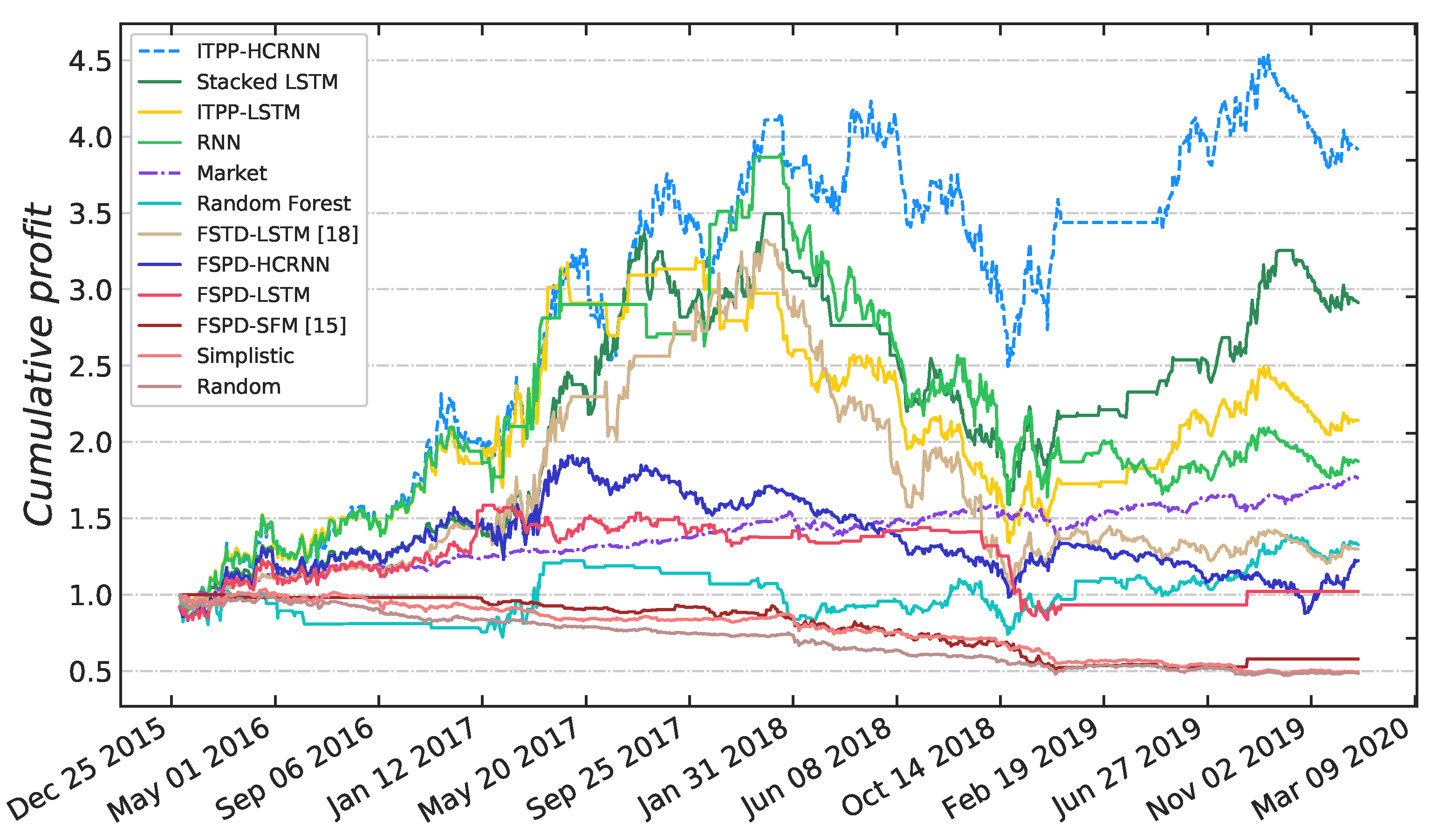
• Discussion of effectiveness: Compared to the performance of simplistic and random methods, all of the other methods show an improvement, suggesting that these methods have a certain predictive ability and are capable of extracting profitable information. Although the performances of FSPD-SFM, FSPD-LSTM, FSPD-HCRNN, FSTD-LSTM, and Random Forest are worse than that of the market (18.99%), an important factor is that the transaction cost offsets the profits. The other four methods earn more profit than the market, and they are all based on our proposed important trading point prediction framework. In terms of the comparison of FSPD-LSTM, FSTD-LSTM, and ITPP-LSTM, the improvement of ITPP-LSTM is indicated by both the annualized return and the Sharpe ratio. It can be concluded that the proposed important trading point prediction framework is indeed effective in stock performance prediction tasks; moreover, it has great advantages over the traditional method of forecasting stock prices directly and forecasting stock trends directly.
• Discussion of the RNN setting: Although Random Forest could obtain some profit, the performance of Random Forest is clearly worse than that of the other RNN-based methods, which is probably because the RNN networks can extract temporal information effectively, but Random Forest does not have this ability. This result indicates the significance of using RNNs for sequential modeling in the context of our research.
• Discussion of the stacked LSTM setting: In contrast to the RNN, LSTM has the ability to maintain the long-term memory of the trading patterns from the historical sequence data; thus, IPTT-LSTM outperforms the RNN. In addition, as stacking LSTM layers can enable the characteristics of raw temporal data to be learned from diverse perspectives at each time step, we can see that stacked LSTM shows certain improvements in the experimental results.
• Discussion of our proposed HCRNN model: Unlike the traditional method, which only utilizes RNNs to learn sequential information, the hybrid neural network we propose combines an RNN and CNN to capture both long-term temporal dependencies and local fluctuation features simultaneously during the training process, as they can complement each other. As we can see from Figure 7, our ITPP-HCRNN significantly outperforms all the above-mentioned models for all the test times. Therefore, we can conclude that such a hybrid neural network can indeed enhance the prediction capability of the method, and utilizing a CNN to extract implicit local fluctuation features can promote accurate prediction.

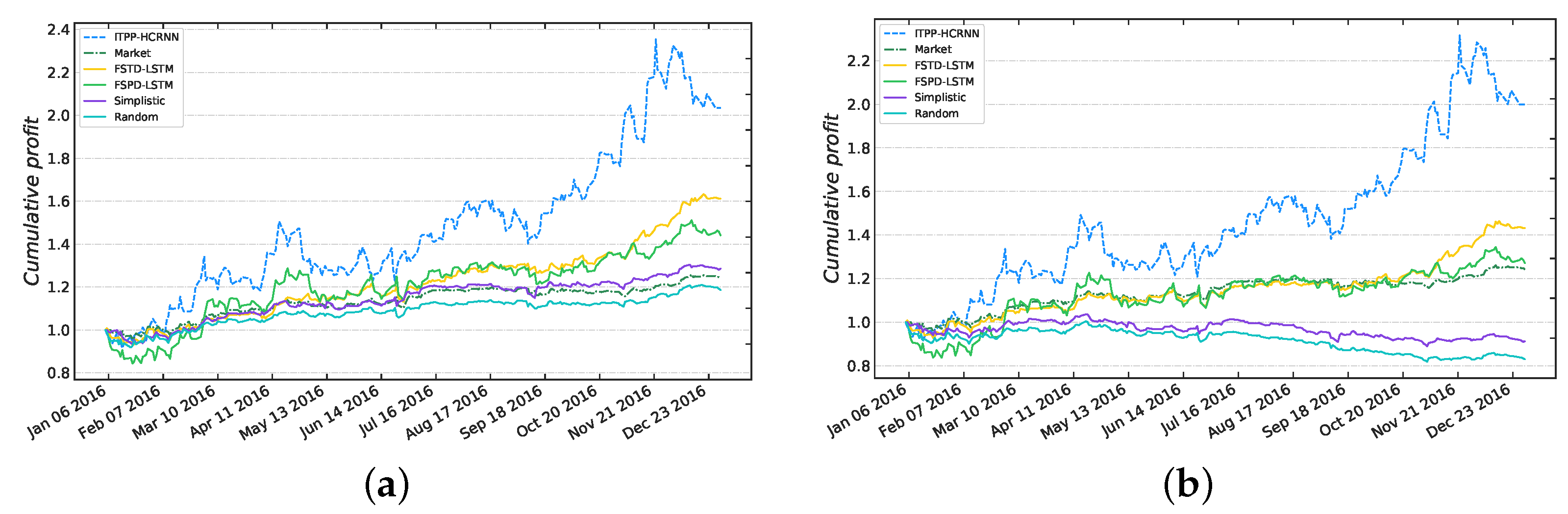
5.3. Impact of Transaction Costs

In reality, transaction costs play a crucial role in the return of an investment strategy. To explore the reasons why the proposed important trading point prediction framework can achieve better performance, we compare the simulation results when considering transaction costs and not considering transaction costs. Figure 8 shows the cumulative profit curves under these two conditions, and the following observations can be found.

If the transaction costs are not considered, all six methods are profitable. Although they are inferior to the proposed method, the other five methods can also earn profits close to the performance of the market. In particular, FSPD-LSTM and FSTD-LSTM are able to earn significantly more profit than the other three methods. Nevertheless, if we consider the transaction costs, the performances of FSPD-LSTM and FSTD-LSTM are not much better than the performance of the market. In addition, simplistic and random methods even obtain negative returns. The reason for this is that these methods make trades too frequently, and the profits are offset by a high number of transaction costs. In contrast, the proposed method focuses only on the important trading points, thus reducing the transaction frequency. As a result, the proposed method is little affected by transaction costs, which has an influential impact on the actual returns.

5.4. Impact of Hyperparameters

Considering that the hyperparameters L and W are important influencing factors (Section 4.1), in this subsection, the effects of different values of L and W are tested to determine the appropriate hyperparameters. The results generated using several representative values are listed in

Table 5. Comparison results of different hyperparameters based on the 2016 dataset, where L in (L, W) is the length of the signal of IPs and W in (L, W) is the threshold of IPs.

(L, W)	(3, 1.05)	(4, 1.05)	(5, 1.05)	(6, 1.05)	(7, 1.05)
Profit ratio	94.30%	105.00%	72.90%	80.90%	92.10%
(L, W)	(4, 1.03)	(4, 1.04)	(4, 1.05)	(4, 1.06)	(4, 1.07)
Profit ratio	44.30%	86.20%	105.00%	104.00%	48.80%

. It can be concluded that the proposed framework shows promising performance with different configurations, and the values (4, 1.05) are better than other values. The reason is as follows: if the length of the signal of IPs L is too long, it is inevitable that the learning process of the underlying patterns of important trading points will be disturbed by more noise. On the other hand, if the length L is too short, it will not be sufficiently long to identify the internal laws of price fluctuation, which will make it difficult for the neural network to make accurate predictions. In terms of the threshold W of IPs, if W is very low, the distinction between important and normal points will not be sufficiently obvious; thus, the neural network will not be able to learn the underlying patterns of important trading points. However, if we set a threshold W that is too high, it will cause the number of detected IPs to be very small and lead to missing some profitable opportunities. As a result, even if the profit of each transaction increases, the total profit may decrease. Therefore, setting a moderate value is more likely to achieve the best performance.

6. Conclusions and Future Work

In this paper, we note three principles in seeking trading opportunities—focusing on high-margin opportunities, keeping track for some time, and diversifying the investment portfolio—by imitating the learning process of human investors. Based on these principles, this study proposes a new deep learning framework—a hybrid convolutional recurrent neural network (HCRNN)—for important trading point prediction in the stock market. In contrast to previous studies, the proposed framework regards trading signals as previous time step sequences instead of a single time step. Then, the signals of important trading points are used to train the HCRNN model to learn the underlying patterns of important trading points. The HCRNN model applies LSTM to capture long-term temporary dependencies from historical stock data time series and utilizes a CNN to extract implicit local fluctuation features to enhance the prediction ability. Extensive experiments on real stock market data demonstrate the superior performance of the proposed model. Specifically, we perform additional fund simulations, and our proposed framework can produce appreciable profits with significantly increased annualized excess returns, which is a remarkable improvement compared to the market performance. Besides, comparison results indicate that focusing on the important trading points which are more likely to be a high-margin opportunity rather than predicting the stock price or trend at every time point can result in more profits due to the uncertainty and difficulty of the stock price forecasting task as well as the considerable transaction costs that make slight price fluctuations meaningless. In summary, this work provides new insights into stock performance prediction research and can help investors to develop better trading systems.

At present, to verify the effectiveness of our approach, we apply only a basic trading strategy, as described in Section 5.2, which does not include a stop-loss strategy (cut losses and let winnings continue). In the future, we plan to leverage more advanced trading strategies. The empirical results reported here are based on the American stock market, we will further verify the effectiveness of the proposed approach in other countries’ stock markets. Furthermore, we will investigate whether retraining the model more frequently, such as by updating the model each month, can result in more accurate predictions to boost profits. In addition, it is also promising to apply the proposed method to more granular trading data, such as hourly or per-minute transaction data.

References

1. Li, L.; Leng, S.; Yang, J.; Yu, M. Stock Market Autoregressive Dynamics: A Multinational Comparative Study with Quantile Regression. Math. Probl. Eng. 2016, 2016, 1285768. [Google Scholar] [CrossRef] [Green Version]
2. Zhang, M.; Jiang, X.; Fang, Z.; Zeng, Y.; Xu, K. High-order Hidden Markov Model for trend prediction in financial time series. Phys. A Stat. Mech. Appl. 2019, 517, 1–12. [Google Scholar] [CrossRef]
3. Song, Y.; Lee, J. Importance of Event Binary Features in Stock Price Prediction. Appl. Sci. 2020, 10, 1597. [Google Scholar] [CrossRef] [Green Version]
4. Akita, R.; Yoshihara, A.; Matsubara, T.; Uehara, K. Deep learning for stock prediction using numerical and textual information. In Proceedings of the 2016 IEEE/ACIS 15th International Conference on Computer and Information Science (ICIS), Okayama, Japan, 26–29 June 2016; pp. 1–6. [Google Scholar]
5. Gao, Q. Stock Market Forecasting Using Recurrent Neural Network. Ph.D. Thesis, University of Missouri–Columbia, Columbia, MO, USA, 2016. [Google Scholar]
6. Rather, A.M.; Agarwal, A.; Sastry, V. Recurrent neural network and a hybrid model for prediction of stock returns. Expert Syst. Appl. 2015, 42, 3234–3241. [Google Scholar] [CrossRef]
7. Hochreiter, S.; Schmidhuber, J. Long short-term memory. Neural Comput. 1997, 9, 1735–1780. [Google Scholar] [CrossRef] [PubMed]
8. Li, H.; Shen, Y.; Zhu, Y. Stock price prediction using attention-based multi-input LSTM. In Proceedings of the Asian Conference on Machine Learning, Beijing, China, 14–16 November 2018; pp. 454–469. [Google Scholar]
9. Fischer, T.; Krauss, C. Deep learning with long short-term memory networks for financial market predictions. Eur. J. Oper. Res. 2018, 270, 654–669. [Google Scholar] [CrossRef] [Green Version]
10. Gu, Y.; Shibukawa, T.; Kondo, Y.; Nagao, S.; Kamijo, S. Prediction of Stock Performance Using Deep Neural Networks. Appl. Sci. 2020, 10, 8142. [Google Scholar] [CrossRef]
11. Bao, W.; Yue, J.; Rao, Y. A deep learning framework for financial time series using stacked autoencoders and long-short term memory. PLoS ONE 2017, 12, e0180944. [Google Scholar] [CrossRef] [Green Version]
12. Sirignano, J.; Cont, R. Universal features of price formation in financial markets: Perspectives from deep learning. Quant. Financ. 2019, 19, 1449–1459. [Google Scholar] [CrossRef]
13. Tsantekidis, A.; Passalis, N.; Tefas, A.; Kanniainen, J.; Gabbouj, M.; Iosifidis, A. Using deep learning to detect price change indications in financial markets. In Proceedings of the 2017 25th European Signal Processing Conference (EUSIPCO), Kos Island, Greece, 28 August–2 September 2017; pp. 2511–2515. [Google Scholar]
14. Li, J.; Bu, H.; Wu, J. Sentiment-aware stock market prediction: A deep learning method. In Proceedings of the 2017 International Conference on Service Systems and Service Management, Dalian, China, 16–18 June 2017; pp. 1–6. [Google Scholar]
15. Zhang, L.; Aggarwal, C.; Qi, G.J. Stock price prediction via discovering multi-frequency trading patterns. In Proceedings of the 23rd ACM SIGKDD International Conference on Knowledge Discovery and Data Mining, Halifax, NS, Canada, 13–17 August 2017; pp. 2141–2149. [Google Scholar]
16. Si, W.; Li, J.; Ding, P.; Rao, R. A multi-objective deep reinforcement learning approach for stock index future’s intraday trading. In Proceedings of the 2017 10th International Symposium on Computational Intelligence and Design (ISCID), Hangzhou, China, 9–10 December 2017; Volume 2, pp. 431–436. [Google Scholar]
17. Hao, Y.; Gao, Q. Predicting the Trend of Stock Market Index Using the Hybrid Neural Network Based on Multiple Time Scale Feature Learning. Appl. Sci. 2020, 10, 3961. [Google Scholar] [CrossRef]
18. Nelson, D.M.; Pereira, A.C.; de Oliveira, R.A. Stock market’s price movement prediction with LSTM neural networks. In Proceedings of the 2017 International Joint Conference on Neural Networks (IJCNN), Anchorage, AK, USA, 14–19 May 2017; pp. 1419–1426. [Google Scholar]
19. JuHyok, U.; Lu, P.; Kim, C.; Ryu, U.; Pak, K. A new LSTM based reversal point prediction method using upward/downward reversal point feature sets. Chaos Solitons Fractals 2020, 132, 109559. [Google Scholar]
20. Chang, P.C.; Fan, C.Y.; Liu, C.H. Integrating a piecewise linear representation method and a neural network model for stock trading points prediction. IEEE Trans. Syst. Man Cybern. Part C (Appl. Rev.) 2008, 39, 80–92. [Google Scholar] [CrossRef] [Green Version]
21. Yin, J.; Si, Y.W.; Gong, Z. Financial time series segmentation based on Turning Points. In Proceedings of the 2011 International Conference on System Science and Engineering, Macau, China, 8–10 June 2011; pp. 394–399. [Google Scholar]
22. Huang, Q.; Yang, J.; Feng, X.; Liew, A.W.-C.; Li, X. Automated trading point forecasting based on bicluster mining and fuzzy inference. IEEE Trans. Fuzzy Syst. 2019, 28, 259–272. [Google Scholar] [CrossRef]
23. Liu, S.; Zhang, C.; Ma, J. CNN-LSTM neural network model for quantitative strategy analysis in stock markets. In Proceedings of the International Conference on Neural Information Processing, Guangzhou, China, 14–18 November 2017; pp. 198–206. [Google Scholar]
24. Dospinescu, N.; Dospinescu, O. A profitability regression model in financial communication of Romanian stock exchange’s companies. Ecoforum J. 2019, 8, 1–4. [Google Scholar]
25. Dospinescu, O.; Dospinescu, N. A profitability regression model of romanian stock exchange’s energy companies. In Proceedings of the IE 2018 17th International Conference on Informatics in Economy Education, Research & Business Technologies, lasi, Romania, 17–20 May 2018; pp. 169–174. [Google Scholar]
26. Atsalakis, G.S.; Dimitrakakis, E.M.; Zopounidis, C.D. Elliott Wave Theory and neuro-fuzzy systems, in stock market prediction: The WASP system. Expert Syst. Appl. 2011, 38, 9196–9206. [Google Scholar] [CrossRef]
27. Hyerczyk, J.A. Pattern, Price and Time: Using Gann Theory in Technical Analysis; John Wiley & Sons: Hoboken, NJ, USA, 2009; Volume 408. [Google Scholar]
28. Sykes, T. The Golden Ratio of Stock Trading. Available online: https://www.wallstreetdaily.com/2019/10/03/the-golden-ratio-of-stock-trading/ (accessed on 26 February 2021).
29. Szegedy, C.; Ioffe, S.; Vanhoucke, V.; Alemi, A. Inception-v4, inception-resnet and the impact of residual connections on learning. In Proceedings of the AAAI Conference on Artificial Intelligence, San Francisco, CA, USA, 4–9 February 2017; Volume 31. [Google Scholar]
30. Li, H. Deep learning for natural language processing: Advantages and challenges. Natl. Sci. Rev. 2018, 5, 24–26. [Google Scholar] [CrossRef]
31. Khan, M.A.; Kim, J. Toward Developing Efficient Conv-AE-Based Intrusion Detection System Using Heterogeneous Dataset. Electronics 2020, 9, 1771. [Google Scholar] [CrossRef]
32. Hu, Z.; Zhao, Y.; Khushi, M. A Survey of Forex and Stock Price Prediction Using Deep Learning. Appl. Syst. Innov. 2021, 4, 9. [Google Scholar] [CrossRef]
33. Yahaya, A.; Abubakar, A.H.; Garba, J. Statistical analysis on the advantages of portfolio diversification. Int. J. Pure Appl. Sci. Technol. 2011, 7, 98–106. [Google Scholar]
34. Goetzmann, W.N.; Kumar, A. Equity portfolio diversification. Rev. Financ. 2008, 12, 433–463. [Google Scholar] [CrossRef] [Green Version]
35. Thakkar, A.; Chaudhari, K. Fusion in stock market prediction: A decade survey on the necessity, recent developments, and potential future directions. Inf. Fusion 2021, 65, 95–107. [Google Scholar] [CrossRef]
36. Zhan, X.; Li, Y.; Li, R.; Gu, X.; Habimana, O.; Wang, H. Stock Price Prediction Using Time Convolution Long Short-Term Memory Network. In Proceedings of the International Conference on Knowledge Science, Engineering and Management, Changchun, China, 17–19 August 2018; pp. 461–468. [Google Scholar]
37. Kim, T.; Kim, H.Y. Forecasting stock prices with a feature fusion LSTM-CNN model using different representations of the same data. PLoS ONE 2019, 14, e0212320. [Google Scholar] [CrossRef] [PubMed]
38. Chen, C.T.; Chen, A.P.; Huang, S.H. Cloning strategies from trading records using agent-based reinforcement learning algorithm. In Proceedings of the 2018 IEEE International Conference on Agents (ICA), Singapore, 28–31 July 2018; pp. 34–37. [Google Scholar]
39. Siripurapu, A. Convolutional networks for stock trading. Stanf. Univ. Dep. Comput. Sci. 2014, 1, 1–6. [Google Scholar]
40. Gunduz, H.; Yaslan, Y.; Cataltepe, Z. Intraday prediction of Borsa Istanbul using convolutional neural networks and feature correlations. Knowl. Based Syst. 2017, 137, 138–148. [Google Scholar] [CrossRef]
41. Wang, Y.; Zhang, C.; Wang, S.; Yu, P.; Bai, L.; Cui, L. Deep Co-Investment Network Learning for Financial Assets. In Proceedings of the 2018 IEEE International Conference on Big Knowledge (ICBK), Singapore, 17–18 November 2018; pp. 41–48. [Google Scholar]
42. Eapen, J.; Bein, D.; Verma, A. Novel deep learning model with CNN and bi-directional LSTM for improved stock market index prediction. In Proceedings of the 2019 IEEE 9th Annual Computing and Communication Workshop and Conference (CCWC), Las Vegas, NV, USA, 7–9 January2019; pp. 264–270. [Google Scholar]
43. Long, W.; Lu, Z.; Cui, L. Deep learning-based feature engineering for stock price movement prediction. Knowl. Based Syst. 2019, 164, 163–173. [Google Scholar] [CrossRef]
44. Chen, J.F.; Chen, W.L.; Huang, C.P.; Huang, S.H.; Chen, A.P. Financial time-series data analysis using deep convolutional neural networks. In Proceedings of the 2016 7th International Conference on Cloud Computing and Big Data (CCBD), Macau, China, 16–18 November 2016; pp. 87–92. [Google Scholar]
45. Sezer, O.B.; Ozbayoglu, A.M. Algorithmic financial trading with deep convolutional neural networks: Time series to image conversion approach. Appl. Soft Comput. 2018, 70, 525–538. [Google Scholar] [CrossRef]
46. Zhou, X.; Pan, Z.; Hu, G.; Tang, S.; Zhao, C. Stock market prediction on high-frequency data using generative adversarial nets. Math. Probl. Eng. 2018, 2018. [Google Scholar] [CrossRef] [Green Version]
47. Bowman, R. Fundamental vs. Technical Analysis—Beginner’s Guide with Pros and Cons of Each Investment Analysis Method. Available online: https://catanacapital.com/blog/fundamental-vs-technical-analysis-beginners-guide/ (accessed on 26 February 2021).
48. Pratt, K.B. Locating Patterns in Discrete Time-Series. Master’s Thesis, University of South Florida, Tampa, FL, USA, 2001. [Google Scholar]
49. Fu, T.c.; Chung, F.l.; Luk, R.; Ng, C.m. Representing financial time series based on data point importance. Eng. Appl. Artif. Intell. 2008, 21, 277–300. [Google Scholar] [CrossRef]
50. Krizhevsky, A.; Sutskever, I.; Hinton, G.E. Imagenet classification with deep convolutional neural networks. Commun. ACM 2017, 60, 84–90. [Google Scholar] [CrossRef]
51. Widiastuti, N. Convolution Neural Network for Text Mining and Natural Language Processing. In IOP Conference Series: Materials Science and Engineering; IOP Publishing: Bristol, UK, 2019; Volume 662, p. 052010. [Google Scholar]
52. Khand, S.; Anand, V.; Qureshi, M.N. The Predictability and Profitability of Simple Moving Averages and Trading Range Breakout Rules in the Pakistan Stock Market. Rev. Pac. Basin Financ. Mark. Policies 2020, 23, 2050001. [Google Scholar] [CrossRef]
53. Chang, E.J.; Lima, E.J.A.; Tabak, B.M. Testing for predictability in emerging equity markets. Emerg. Mark. Rev. 2004, 5, 295–316. [Google Scholar] [CrossRef]
54. Chen, J. The Anatomy of Trading Breakouts. Available online: https://www.investopedia.com/articles/trading/08/trading-breakouts.asp (accessed on 26 February 2021).
55. Mitchell, C. Breakout Definition and Example. Available online: https://www.investopedia.com/terms/b/breakout.asp (accessed on 26 February 2021).
Figure 1. An example of the lagging phenomenon: prediction results for the S&P500 index from August 2017 to September 2018 using a long short-term neural network.
Applsci 11 03984 g001
Figure 2. Example of a stock breakout.
Applsci 11 03984 g002
Figure 3. Four examples of bullish candlestick patterns.
Applsci 11 03984 g003
Figure 4. Structure of the proposed hybrid convolutional recurrent neural network (HCRNN) model for important trading point prediction, where detailed layer connections are indicated.
Applsci 11 03984 g004
Figure 5. The flow chart of the proposed important trading point prediction framework based on a hybrid convolutional recurrent neural network (HCRNN).
Applsci 11 03984 g005
Figure 6. The F1 score results for different models. RF: random forest; RNN: recurrent neural network; ITPP: important trading point prediction; LSTM: long short-term memory; HCRNN: hybrid convolutional recurrent neural network.
Applsci 11 03984 g006
Figure 7. The cumulative profit curve for each method over four years.
Applsci 11 03984 g007
Figure 8. Impact of transaction costs. Transaction costs are not considered in (a). Transaction costs are considered in (b).
Applsci 11 03984 g008