Article

The Limitations of 5f Delocalization and Dispersion

1
Departments of Physics and Chemistry, University of Wisconsin-Oshkosh, Oshkosh, WI 54901, USA
2
SLAC National Accelerator Laboratory, Menlo Park, CA 94025, USA
3
Lawrence Livermore National Laboratory, Livermore, CA 94550, USA
*
Authors to whom correspondence should be addressed.
Appl. Sci. 2021, 11(9), 3882; https://doi.org/10.3390/app11093882
Submission received: 31 December 2020 / Revised: 19 April 2021 / Accepted: 22 April 2021 / Published: 25 April 2021

Abstract

:
Delocalization in the 5f states of the actinides is an important phenomenon, but poorly quantified. Here, the fundamental limitations of 5f dispersion measurements using angle and momentum resolved variants of photoelectron spectroscopy will be discussed. A novel approach will be suggested, based on a theoretical projection, which should circumvent these limitations: M4,5 X-ray emission spectroscopy. This analysis will utilize the case study of U metal, which can be considered to be the paramount example of 5f dispersion.

1. Introduction

In many respects, it is the delocalization of the 5f states that sets them apart from 4f behavior. One very powerful aspect of 5f delocalization is the size dependence of the actinides with fillings, as can be seen in Figure 1 below. In the early part of the series, the size dependence is much more like a 5d filling than a 4f filling. This observation has been known and reported on for many years [1,2,3]. In fact, it temporarily led to the erroneous hypothesis that the actinide series was a 6d filling series [4,5]. It is only as the 5f states fill further that the impact of the jj-skewed intermediate coupling of 5f angular momenta becomes clear, with a dramatic change in both the atomic size (lower panel) and angular momentum coupling (upper panel) [6,7,8]. Interestingly, it is the nature of the 5f intermediate coupling that is the other major difference between 4f (Russell–Saunders skewed) and 5f (jj skewed) behavior. This subject will be revisited and further explored later in the discussions herein.
From a consideration of the results in Figure 1, it is clear that perhaps the best example of 5f delocalization is U metal. The atomic size dependence near U is still in the 5d-like regime and the angular momentum coupling has diverged from the predictions of the intermediate coupling model [6,7,8,9], which is based upon a picture assuming a high degree of localization in the 5f states. Furthermore, U metal has been the subject of many investigations and extensive data concerning its electronic structure already exist. An example of this is shown in Figure 2. Thus, the analysis in this paper is not a review of the field but rather a detailed case study with extensive prior investigations.
There is a remarkable level of agreement between the earlier measurements of Baer and Lang [14,15] and the theory from Kutepov et al. [8,16,17]. The X-ray Photoelectron Spectroscopy (XPS) and Bremsstrahlung Isochromat Spectroscopy (BIS, a type of high energy inverse photoelectron spectroscopy) provide a good measure of the occupied (ODOS) and unoccupied (UDOS) density of states, respectively. Effectively, the XPS and BIS are angle and momentum averaging results. However, to gain a further understanding of the electronic structure, more discerning measurements are desirable. The logical choice is angle resolved photoelectron spectroscopy, ARPES, for several reasons. (1) In general, photoelectron spectroscopy has far higher counting rates than inverse photoelectron spectroscopy, on the order of ×10,000 [18]. (2) ARPES has a strong track record of success in the determination of momentum of resolved electronic structures [19,20,21,22,23]. (3) Single crystals of U are available [24,25]. It will be shown that ARPES has significant limitations in its application to U and that other approaches are more effective. However, before considering the extant ARPES results for U, it is useful to define some of the experimental conditions and review some cases of successful analyses with ARPES. Thus, the sections that follow are: Section 2—experiment; Section 3—digression on ARPES; Section 4—ARPES of U; Section 5—X-ray absorption spectroscopy (XAS); Section 6—X-ray emission spectroscopy (XES); and Section 7—the summary.

2. Experimental Section

Photoelectron spectroscopy (PES) and inverse photoelectron spectroscopy (IPES) or Bremsstrahlung isochromat spectroscopy (BIS) can be used to measure the energy of the electronic states immediately below (PES) or above (IPES/BIS) the Fermi energy. If the direction of the electrons involved in either process is defined, it is possible to measure the dispersion relations of these states, i.e., energy versus momentum. The variant of PES that allows this is ARPES, angle resolved photoelectron spectroscopy, because the emission direction of the electrons is restricted via angular resolution of the collected electrons. Of course, both the electrons and photons must be monochromatized in some sense, with a small energy range. Generally speaking, the momentum parallel to the surface is conserved and the momentum perpendicular to the surface is determined via energy conservation and the assumption that the final state is plane-wave-like [18,19,20,21,22,23].
The X-ray emission and absorption spectroscopy (XES and XAS) measurements were carried out at the Stanford Synchrotron Radiation Lightsource (SSRL), the particulars of which are described elsewhere [17,26,27]. The details of the other experiments and calculations can be found in the source articles, quoted in the text and cited as references below. In general, it should be noted that actinides are highly reactive. The lifetime of an atomically clean metal actinide surface in ultra-high vacuum (10–10 to 10–11 Torr) is on the order of a couple or few hours [28]. Electron-based techniques, with short penetration and/or escape depths, are especially surface sensitive, but even M edge spectroscopy (hv ~ 3 keV) have been demonstrated to exhibit an enhanced surface sensitivity relative to the higher energy (hv ~ 17 keV) measurements [29]. However, it is important to differentiate that what is meant as a “surface” for the electron-based spectroscopies is typically the first couple of atomic layers, whereas what is meant as a “surface” in photon-out spectroscopies, e.g., for M-edge XAS, is on the order of 10 s to 100 s of nm—which is substantially larger, penetrating far deeper into the material [29].

3. Digression on ARPES
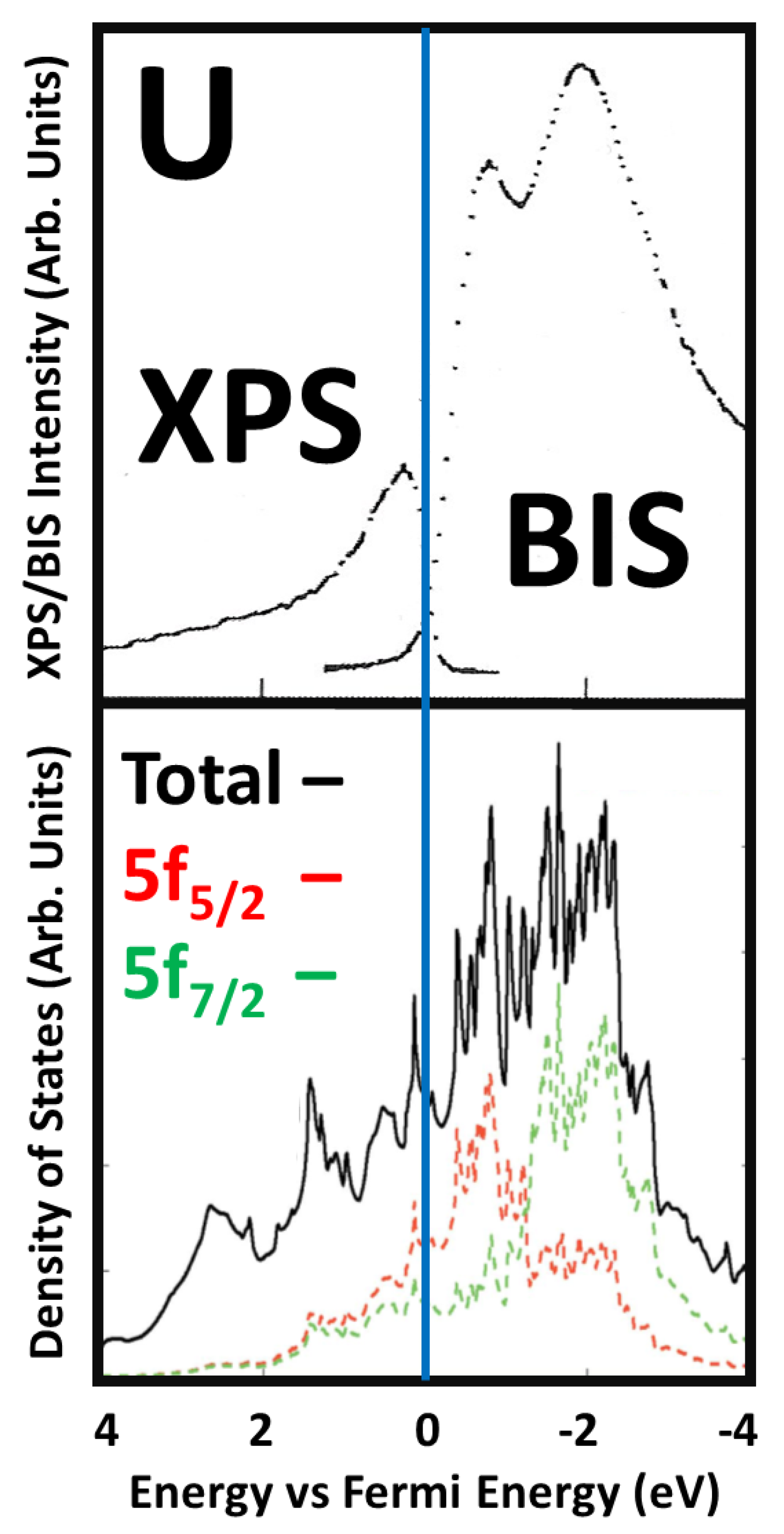
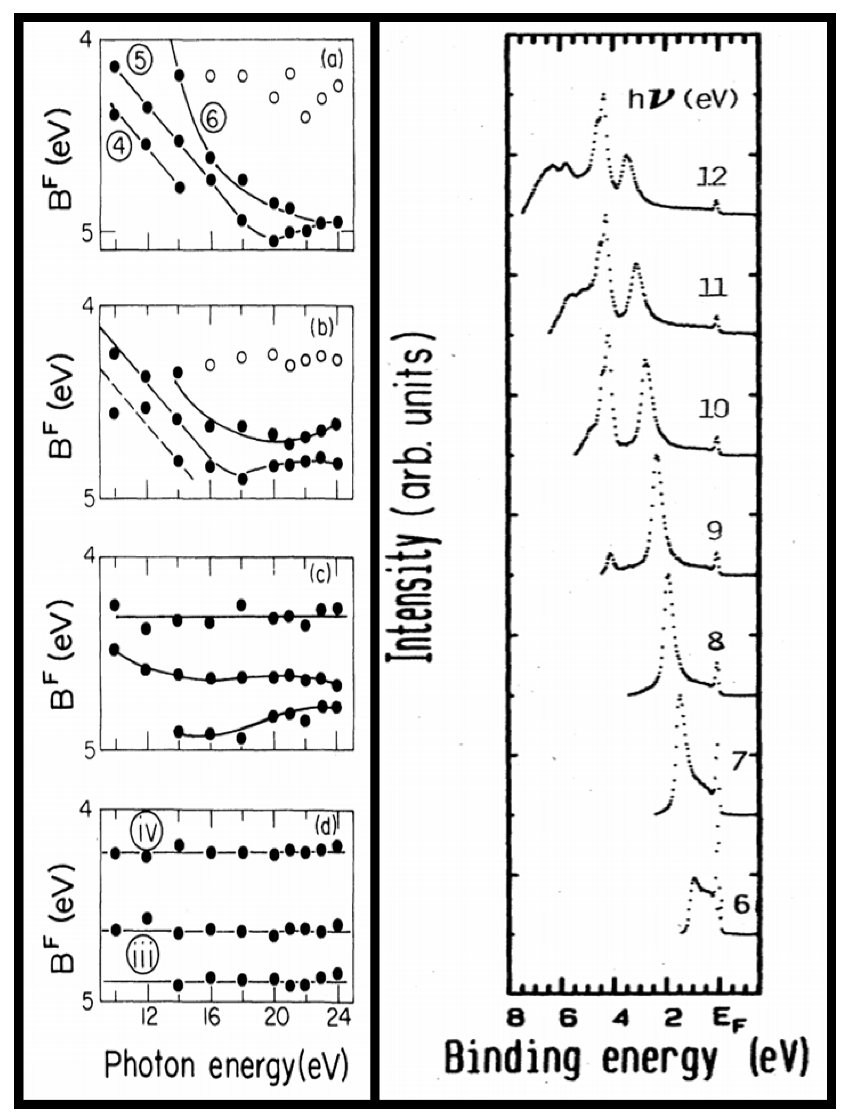
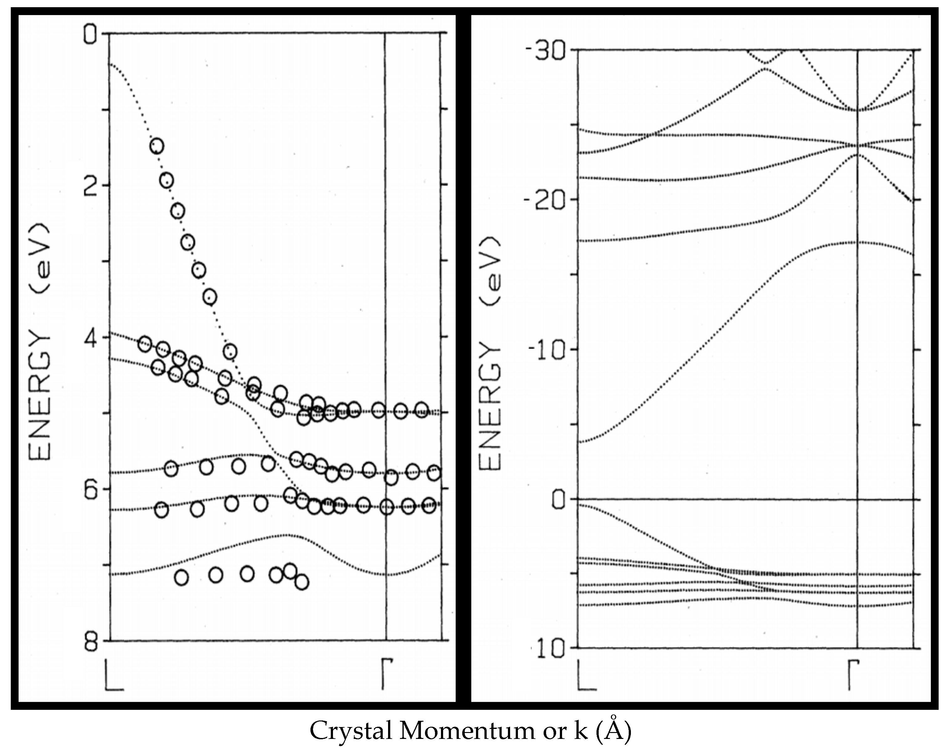
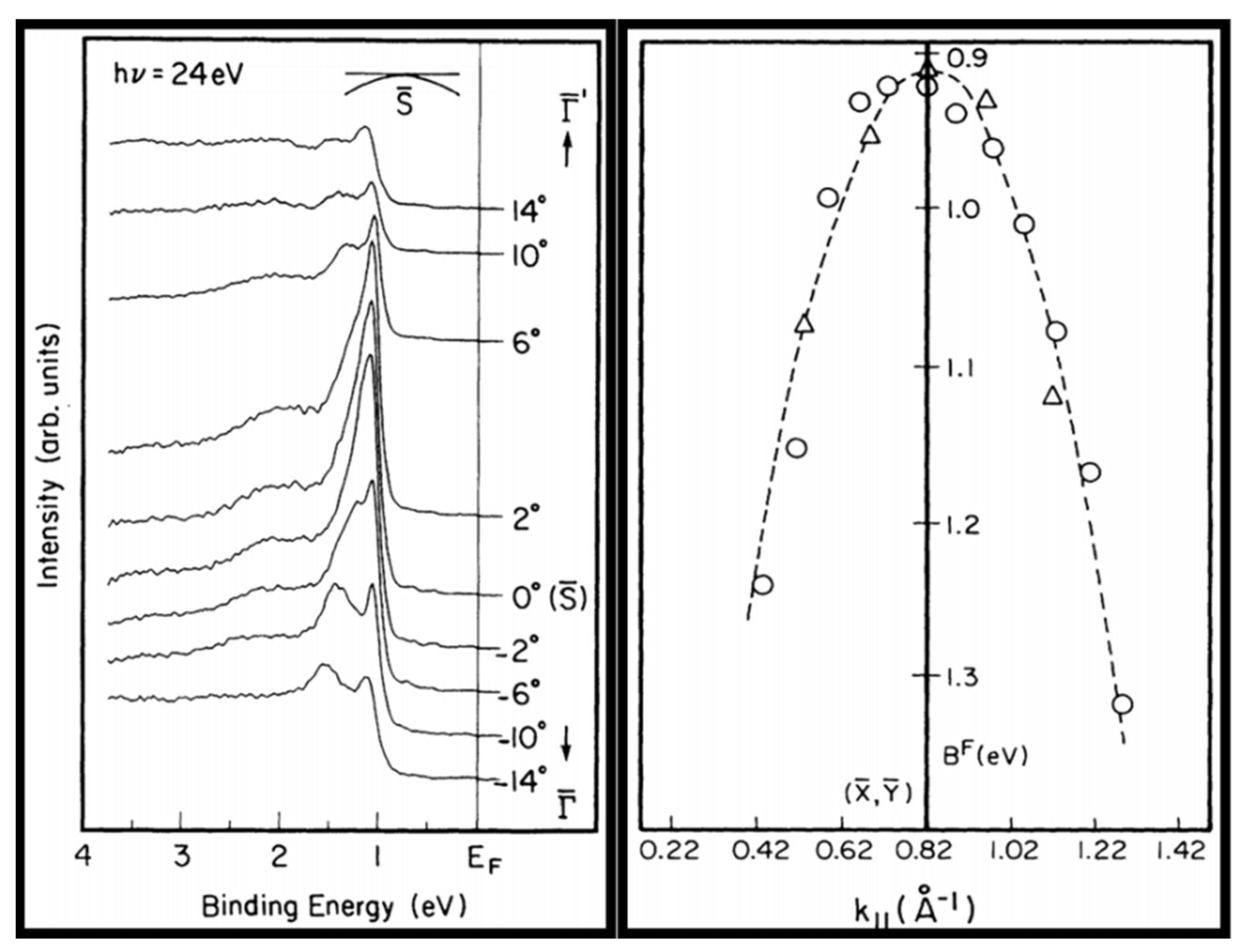
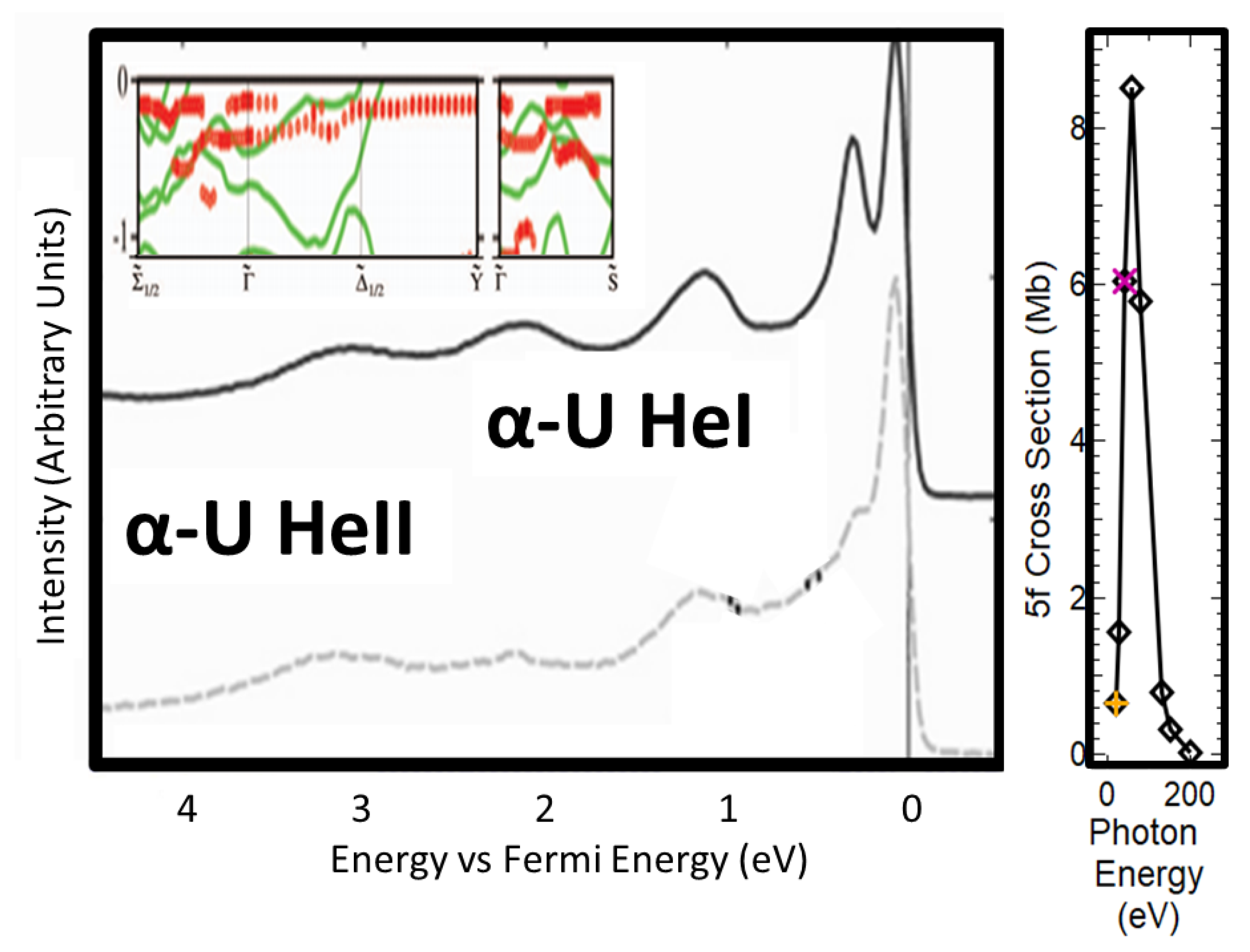
It is useful to remember that, in the Hamiltonian of the Schrödinger Equation, it is the symmetry of the potential that determines the symmetry of the solutions, i.e., the wavefunctions [30]. Thus, a periodic lattice will give rise to periodic wavefunctions, dependent upon the linear or translational crystal momentum. Hence, in many respects, ARPES is the perfect tool with which to probe the electronic structure of an ordered lattice. Examples of this abound, but one of particular application here is the system of Ag/Cu(001) and Ag(111) [19,20,21,22].
In Figure 3 is shown a summary of an extensive study that demonstrated the development from 2-D, in plane, dispersion to 3-D dispersion, as the thickness of the silver overlayer was increased from one monolayer (ML) to five monolayers, with convergence to behavior very similar to bulk Ag(111) [19,20,21,22]. This case is clearly an example of strong delocalization and dispersion, evidenced by the movement of the peaks over several eV as the photon energy is increased from 6eV to 12 eV, corresponding to a movement from near its edge (L, hv = 6 eV) to approximately halfway (hv = 12 eV) to the center of the Brillouin zone (Γ), see Figure 3 and Figure 4.
The dispersion of several eV is completely consistent with the most fundamental of models. If one assumes a free electron with KE = ½ mv2, a de Broglie wavelength of λ, and a 1-D periodic chain of atoms with a spacing of d, it can be shown that the electron states will have an energy difference of ~10 eV for d = 2 Å, ~4 eV for d = 3 Å and ~2 eV for d = 4 Å, between the center of the first Brillouin zone (BZ) and its boundary [31].
An important aspect of the analysis of the Ag(111) was the success of an interpolation scheme to model the electronic structure [20]. Here, the 4d states are treated as almost constant features, which then interact with the overlying 5s wave. The states mix and repel, based upon symmetry, giving a high level of agreement with the experimental measurements, as shown in Figure 4. This issue will be revisited below.
Before returning to uranium, it is worthwhile to consider ARPES in a more complex system than Ag(111). Below, in Figure 5, are shown the spectra and dispersion curves for the “1 eV” state in twinned and un-twinned, single crystalline YBCO [23]. The dispersion is smaller than in Ag(111) but easily definable and with a range of several tenths of an eV, and centered upon a high symmetry line in the complicated BZ of YBa2Cu3O6.9. These observations will be utilized and applied in the analysis of the ARPES of α-U that follows in the next section.

4. ARPES of α-U

Metallic α-U has been studied by Opeil et al. [24,25], using angle resolved photoelectron spectroscopy [32], to probe a single crystal of α-U. Examples of their data are shown in Figure 6. These spectra can be compared to those reported earlier in the 1970s and 1980s. It should be noted that Opeil’s spectra are significantly different than those for UO2 [15,33,34], but quite consistent with those for α-U [15,33,35]. This strongly suggests that their data are valid. Nevertheless, it is likely that the surface in these studies was not as clean as asserted. Here are three reasons. (1) XPS has a sensitivity problem with the O1s. This makes it difficult to accurately assess how clean or dirty a sample was based solely on the O1s XPS, because low coverage yet potentially significant levels of O contamination might not be detected (see Figure 6 of Reference [32]). (2) The peak at −5 eV binding energy (Figure 4 of Reference [25]) has been identified as oxygen derived (see Figure 7 of Reference [32]). There are also papers on U that have a similar assignment [15,33,34]. (3) The peak between the 6p3/2 and 6p1/2 is probably oxygen as well (see Figure 5 of Reference [24] and Figure 10 of Reference [32]). However, this level of oxygen contamination may not be sufficient to invalidate the ARPES experiment, only complicate it. Assuming that the sample is still clean enough and the band-mapping valid, an important conclusion can be drawn: the U 5f levels show little if any dispersion and exhibit no clear dependence upon symmetry points in the BZ. Consider what can be gleaned from Figure 6 (the Fermi energy is at 0 eV).
First, examine the angle resolved spectra shown in Figure 6, for excitation with HeI (hv ~21 eV) and HeII (hv ~41 eV) radiation and with normal emission. It is well known that the 5f cross section rises dramatically between hv = 21 and 41 eV, as shown in the right panel of Figure 6, using data from the calculations by Yeh and Lindau [36]. Thus, any 5f derived peak should show a substantial rise between hv = 21 eV and hv = 41 eV. This only occurs for the peaks adjacent to the Fermi level. A careful examination of the spectra leads to two observations: (1) the peak immediately adjacent to the Fermi level (BF ~0 eV) is clearly of predominantly 5f character; (2) the peak at binding energy of ~ ⅓ eV does not rise as substantially, but still may be of 5f character. The assignment of these two peaks as 5f is supported by comparison with Kutepov’s calculations in Figure 2, where a pair of peaks is observed below the Fermi energy, although extending away more from the Fermi energy than is reported experimentally. An important observation is that the two peaks near the Fermi energy, both of 5f character, do not disperse with hv and thus do not disperse with k. Under the conditions of normal emission, k = 0 and k = k. Changing hv under these conditions keeps k constant and only varies k. Hence, this is a test, albeit a fairly rough and incomplete one, of the possible dispersion with k. The result is that no dispersion with k is observed. The k dependence is addressed in the insets. A further consideration of the pseudo three-dimensional mapping in the upper insets clearly shows that the peaks nearest the Fermi level (1) do not disperse significantly or systematically with k, (2) do not behave symmetrically around high symmetry lines in the BZ and (2) do not agree with theory. Thus, ARPES does not provide the desired fingerprint of 5f delocalization, even in single crystal α-U. In fact, better agreement could be obtained with a theoretical approach analogous to the Interpolation Theory discussed above, with two horizontal lines for the pair of potential 5f state families, at ~0 eV (~1 e- per atom, ½ filled for double degeneracy) and ~⅓ eV (2e- per atom, filled for double degeneracy).
Is there an alternative to ARPES that could provide the desired information concerning the degree of 5f delocalization? Below, it will be demonstrated that M edge XES may provide such a probe, but first it is necessary to consider the nature of the interplay of angular momentum coupling and other perturbations in the actinides.

5. X-ray Absorption Spectroscopy: Angular Momentum Coupling and Perturbations

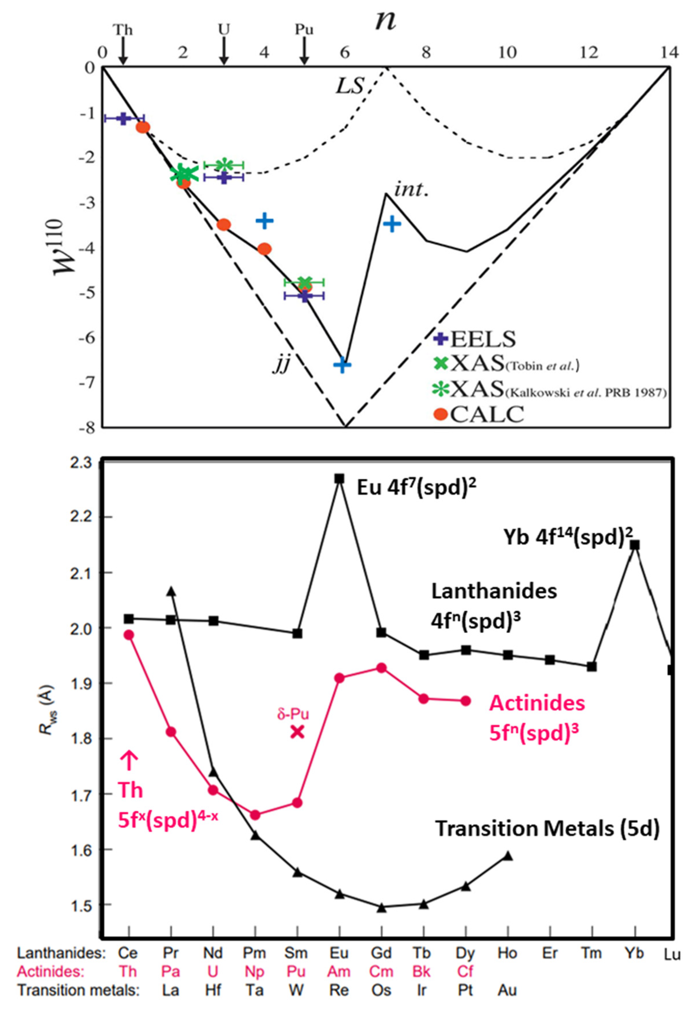
5.1. jj Skewed Intermediate Coupling in the Actinide 5f States

As mentioned briefly above, the other major difference between 4f and 5f behavior is the observation of jj-skewed intermediate coupling in the 5f states. Perhaps the simplest and best illustration of these effects is shown in Figure 7. Here, the jj-skewed intermediate coupling manifests itself as a severe reduction in the intensity of the N4 (4d3/2) XAS peak and the absence of a pre-peak in the O4,5 (5d3/2,5/2) XAS spectrum, in Pu. Note how much different the Pu spectra are from the corresponding UO2 spectra. UO2 is a fairly well-behaved case of a localized, n = 2 system, where n is the number of 5f electrons [10]. Pu is also localized, but with n = 5 [6,7,8]. The proximity to the n = 6 filling of the 5f5/2 manifold, as opposed to the half-filling of the 4f manifold at n = 7, is what causes this strongly variant behavior in Pu. One can also see manifestations of these effects in Figure 1, where the change in behavior in the 5f plot is associated with n = 6. On the other hand, the divergent behavior in the 4f volumes is associated with the preemptive loss of the spd trivalence ((spd)3) so as to obtain either half-filling (4f7) or complete filling (4f14) with spd divalence ((spd)2) [37].

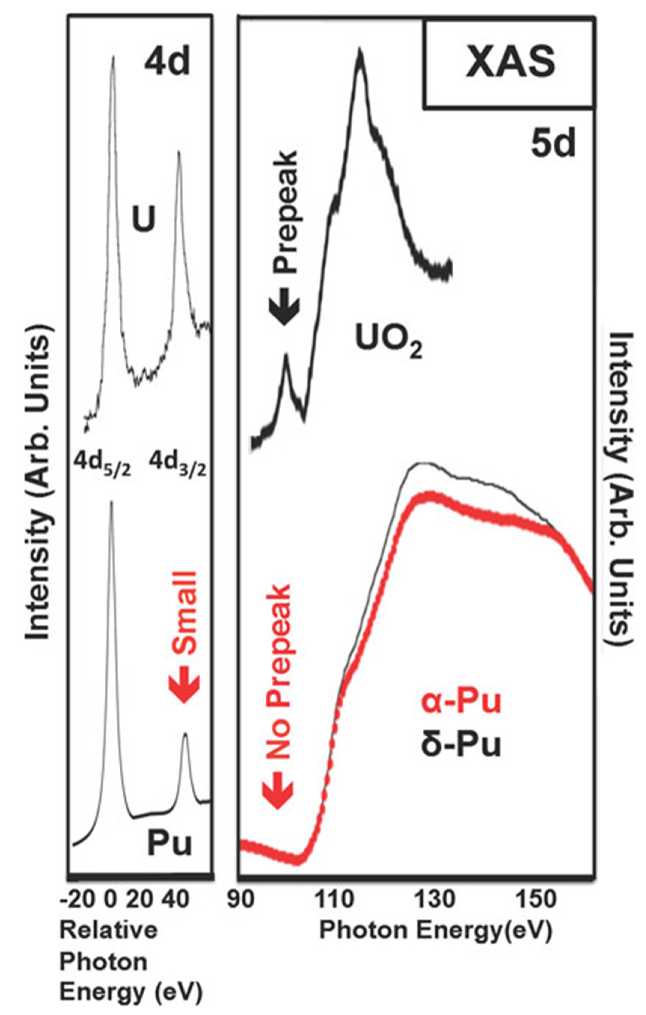
5.2. Prepeak Structures in 4f and 5f Systems

The observation and explanation of the pre-peak structure is not new. In fact, it goes back to 1971, with the theoretical analysis of the pre-peak structure in Ce by Dehmer et al [39], a copy of which is shown in Figure 8. These results will be utilized further in the discussion that follows. The important point for Pu is that in the XAS final state, n increases from 5 to 6, filling the 5f5/2 manifold, eliminating the angular momentum coupling in the final state and thus also preventing any pre-peak structure [6,40].
It is also important to note that the electric dipole selection rules that govern these transitions are founded upon the utilization of spherically symmetric states, i.e., the spherical harmonics [6,7,8,9]. The high level of agreement in Figure 1 between the experimental results, derived from the Branching ratio measurements, and the Intermediate Coupling Theory requires strongly spherically symmetric wavefunctions, for both the core states and the 5f states. Again, the symmetry of the potential determines the symmetry of the solution. The non-spherical perturbations of the 5f states must be weak compared to the spherical potential terms. (Regarding Figure 7: The pre-peak has also been observed for U but the situation for U is complicated by the delocalization. For n = 3, U should have a bigger branching ratio than is observed. This is discussed in detail elsewhere [6,7,8,32]).

5.3. Crystal Field Modifications of Spherically Symmetric Systems

At this point, it is a useful exercise to consider how a potential of non-spherical symmetry would affect angular momentum coupling. To begin, consider a hypothetical situation with a single 5f electron, having both orbital and spin angular momentum, to which is applied a crystal field potential. In this hypothetical case, the crystal field is defined such that Ecfm = |m|Ecf, where m is the magnetic quantum number of the 5f spherical harmonic. This case has been solved before in Reference [42] and utilized in Reference [43]. Briefly, the non-spherically-symmetric crystal field potential and the spherically symmetric spin-orbit interaction are treated on an equal basis within a single particle model. The wave functions are orthogonalized, producing solutions that are dependent upon the relative size of the two potentials. In Figure 9 are a series of plots for several different values ΔEso and Ecf, where ΔEso = (7/2)ζ and ζ (zee) is the 5f spin-orbit splitting parameter. Again, this is a hypothetical case with a simplistic perturbation.
In the upper left-hand panel, the case for ΔEso = 1 eV is shown. This roughly corresponds to U, as can be seen in Figure 2, where a spin orbit splitting of about 1 eV can be observed. It is of interest that in this case, as Ecf increases to values on the scale of 1 eV, there is substantial mixing of the pure 5f7/2 and 5f5/2 states. This means that reasonable values of a crystal field splitting should ruin the selectivity of the electric dipole selection rules that underlie the XAS results of Figure 2 and Figure 7. This result would seem to suggest that crystal field splitting must be much smaller than 1 eV. However, there is a complication.
In the lower panels, the cases associated with a much smaller ζ (ΔEso = 0.1 eV) and larger ζ (ΔEso = 10 eV) are shown. For a smaller ζ, the convergence to the crystal field driven states is almost immediate. The small ζ case would correspond to the conditions of Russell–Saunders (RS) Coupling, going towards the limit of a vanishingly small ζ. This brings home an important point: in general, RS coupling generates states that are consistent with crystal field splitting and require less mixing; but jj coupling is inconsistent with crystal field symmetries and substantial mixing may be required, with a concomitant change in spectral features. For the larger ζ, it is clear that even for the larger Ecf values near 2 eV, the states are still in the first order perturbation limit, where the state energies vary linearly with Ecf and there is not yet significant state mixing between the 5f7/2 and 5f5/2 states. The large ζ case has the advantage that in the case of the conventional XAS shown in Figure 7, the electric dipole selection rules would continue to hold within the intermediate coupling model. That is because, with the large lifetime broadenings, the intensity measurements will average over the entire spectrum and the underlying fine structure will be lost but the cross-sectional dependences would survive. Nonetheless, from the results of Figure 2, it is clear that ζ ~1 eV, not 10 eV.
However, it is not the value of ΔEso that Ecf must overcome, but rather the coulombic repulsion energies, such as those that drive the energy separation in Figure 8 [43]. The spreads of pre-peak structure over the range of 10 eV is caused by the differences in coulombic repulsion associated with different total angular momentum states. It is this type of energy that needs to be overcome by Ecf. Thus, an approximation to the actual situation may correspond to something like that shown in the upper right panel, where the states from ΔEso = 10 eV have been shifted to align with the initial values of ΔEso = 1 eV. This gives us the case of a first order perturbation with linear variations of the energies with Ecf and very little mixing, but centered upon a pure spin-orbit splitting case of ΔEso = 1 eV.
One quirk of this analysis is that it appears that the combination of jj coupling and a first order perturbation from the crystal field gives rise to a mixing of the 5f7/2 and 5f5/2 states much like the results of the intermediate coupling model. Further work is required to quantify this hypothesis.
Our simple model is a single electron picture and real systems, such as uranium dioxide and metallic Pu, are multi-electronic and involve complicated angular momentum coupling. Nevertheless, the same trends should follow in multi-electronic systems. Russel–Saunders or LS coupling involves summing the orbital angular momenta first, followed by coupling to the sum of the spins. Generally, the spin-orbit interactions are smaller, tending towards zero in the limiting case. The sum of the orbital angular momenta should usually be dominant and the solution states should retain the fundamental property of being labile to separation into components consistent with the crystal field, with less extensive mixing required. On the other hand, jj coupling involves summing the spin and orbital components first, then summing the individual electron sums into the total angular momentum. The spin-orbit interaction tends to be larger. The crystal field will need to overcome the spin-orbit splitting interaction, enforced by the coulombic repulsion, whether for a single electron or multiple electrons in order to drive extensive mixing of 5f5/2 and 5f3/2 states. Thus, the mixing of the different j states will be strongly hindered and limited. The upshot of this is that Hund’s Rules [31], which are so powerful in the Russell–Saunders limit, become more like guidelines in jj coupling.

5.4. Brief Digression on Spin-Orbit Splittings and other Measurements

Before going on, it is useful to consider the general trends of spin-orbit splittings throughout the periodic table [44,45,46,47]. It is a common practice in organic chemistry and the studies of small molecules to speak of sp3 (single bonds, tetrahedral symmetry), sp2 (double bonds, trigonal and planar symmetry) and sp (triple bonds, linear symmetry) hybridization [48]. This hybridization works in part because of the relatively low magnitudes of spin-orbit splittings in these cases. Figure 10 shows a tabulation of various spin-orbit splittings for the atoms at the completion of filling of some orbital angular momentum levels. For the 2p, 3p and 3d, the spin-orbit splittings are about 0.1 to 0.2 eV. Similarly, the extrapolation of 4f values in the rare earths indicates that for the early rare earths, the splittings are also small. However, the actinides are different, with values near 1 eV, more similar to the completion of the 4d and 5d series. The Fano measurements [45,46,47] provide a means to probe the spin-orbit splitting, as shown by the examples for Au(111) and Pt(001). The energy splitting in Ce is smaller, consistent with the extrapolation from transition metals back through the rare earths.

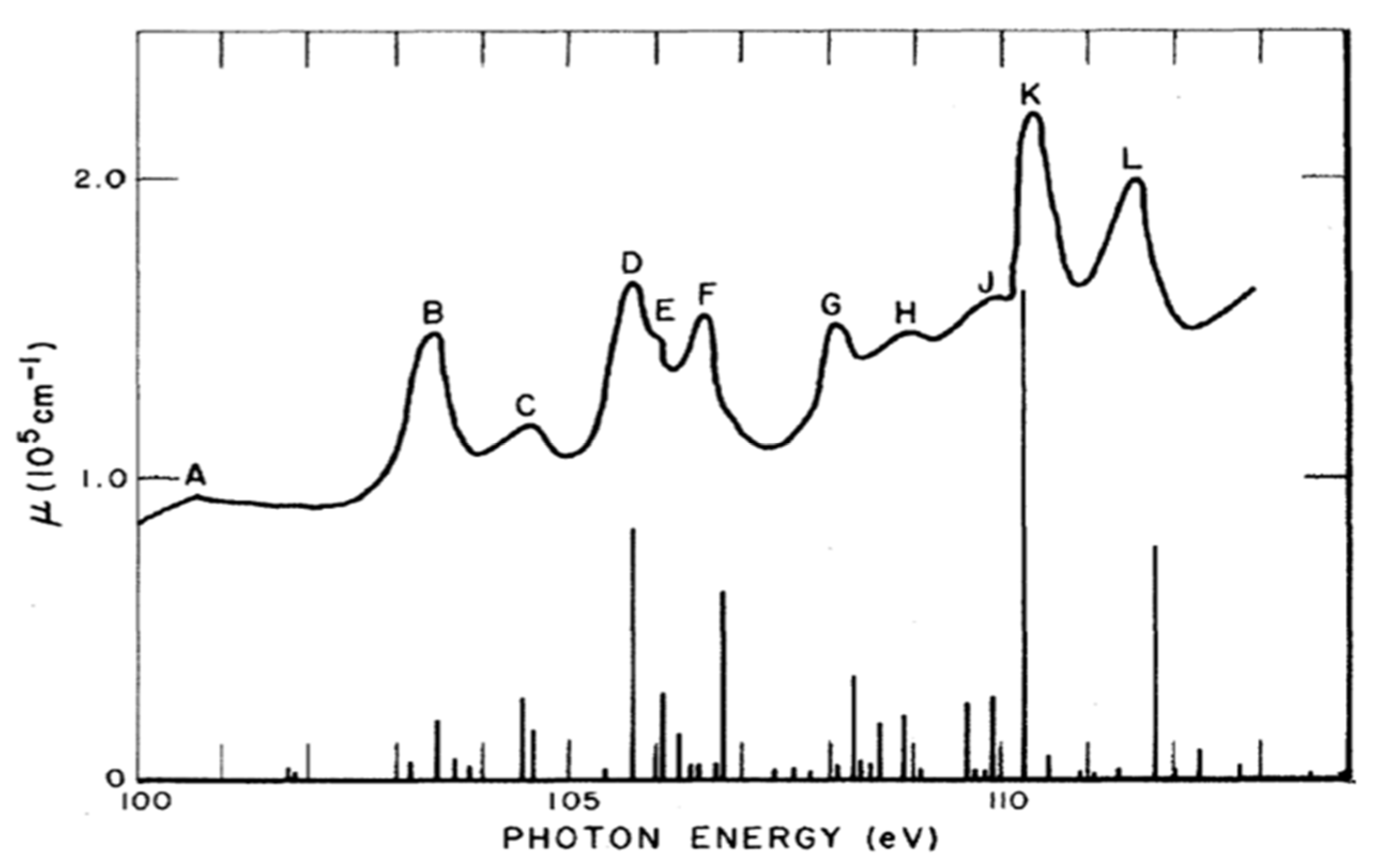
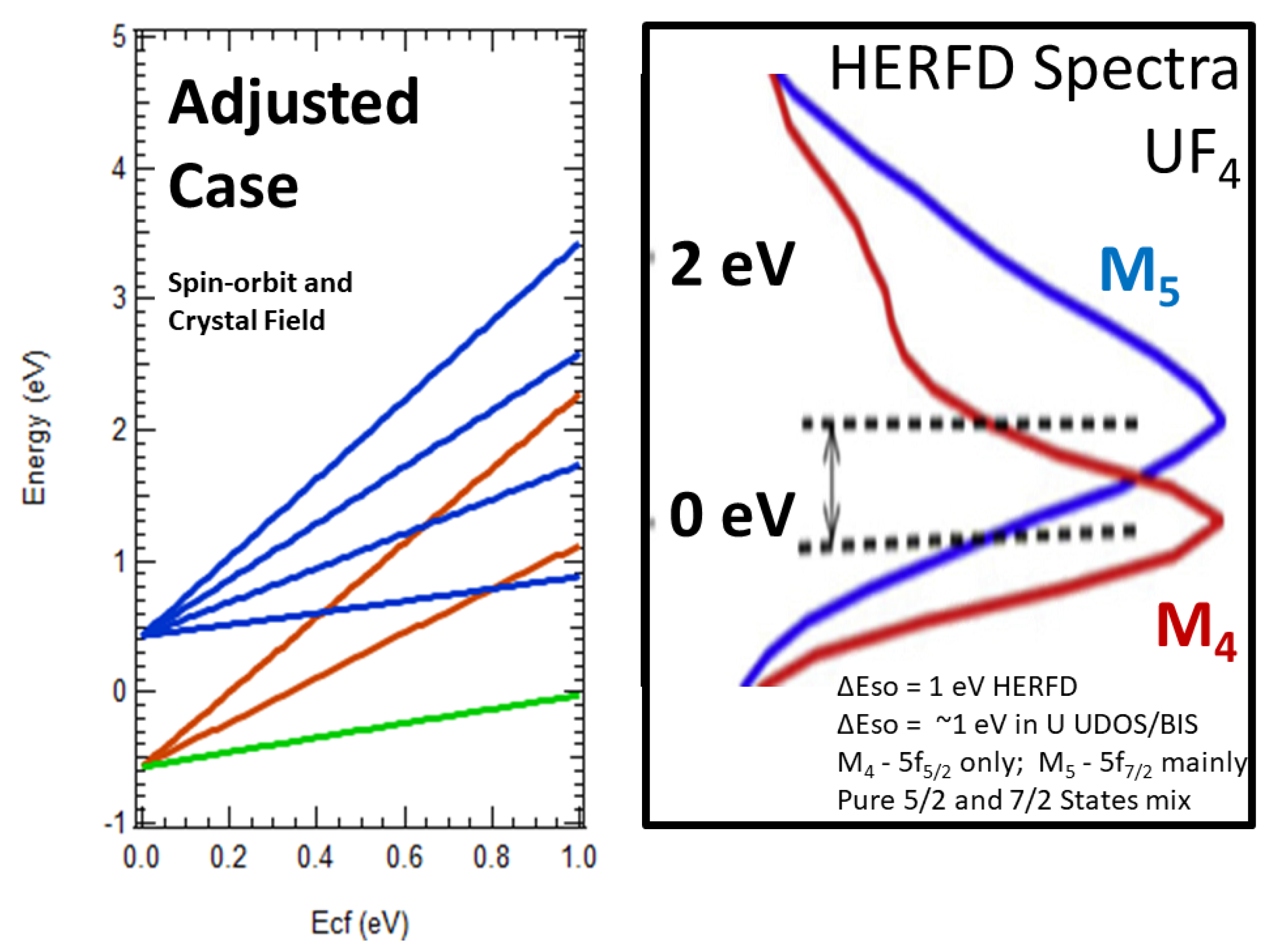
5.5. Evidence of Crystal Field Splittings in HERFD/XAS

Returning to the central argument, the hypothetical case in Figure 9 very roughly corresponds to the situation in UF4, at least in a qualitative fashion. The monoclinic symmetry of UF4 allows only doubly degenerate groupings of states and UF4 is clearly localized and without the dispersion that one might expect from a metallic system. Thus, for illustrative purposes only, it is useful to compare the new high energy resolution fluorescence detection (HERFD) spectra for UF4 [43] with the projection from Figure 9. (Note: HERFD is able to achieve higher resolution by monitoring other decay channels than those that dominate conventional XAS. The result is very high resolution XAS. See Reference [43] for more detail.) This comparison is presented in Figure 11.
The selection rule for the M4 (3d3/2) peak is very strong: 3d3/2 → 5f5/2 only. There is a similar but weaker selection rule for the M5 (3d5/2) peak: 3d5/2 → 5f7/2 mainly [43]. Thus the M5 peak is broader and more featureless than the M4 peak. The M4 peak clearly shows the underlying structure predicted by the model from Figure 9; not so for the M5 peak. However, even the broader M5 peak is consistent with the envelope suggested by the first order perturbation model.
If one considers the possible point group symmetries, in general the cases will correspond to situations similar to those above: a series of doubly degenerate states. The only exception appears to be octahedral/cubic symmetry as in UO2. Thus, in general, the 5f electronic structure of uranium materials should have a series of doubly degenerate states or bands [42,43]. This is also consistent with Kutepov’s ODOS calculation in Figure 3 and the Opeil experiment in Figure 6, for U metal with n = 3: a sharp peak right at the Fermi energy (the half-filled second pair) and a broader peak nearby, BF ~ ⅓, with an occupancy of 2, for a total of 3 electrons of 5f character.

5.6. Implications for Cubic Functions

Finally, a comment on 5f cubic functions needs to be made. It is possible to take linear combinations of the 5f spherical harmonics and produce beautifully symmetric wave-functions of octahedral/cubic symmetry, the so-called cubic functions. These wave-functions can be found in texts on group theory such as that by Cotton [49]. and various websites [50]. Because of the attractiveness of these images and the beauty of the mathematics, they have been utilized in reviews of 5f behavior. Unfortunately, this is very misleading. In order to observe these types of wave-functions, it would be necessary to have crystal fields on the order of 100 eV, so that the coulombic repulsion energies that underlie the intermediate coupling model would be rendered negligible.

6. X-ray Emission Spectroscopy: A New Approach for the Quantification of Mixing

Recently, it has been shown that M4,5 XES of UF4 exhibits manifestations of the same powerful electric dipole selection rules as the N4,5 XAS of the actinides [26]. Here, because of the wide separation of the M4 and M5 edges, the scaling must be done through a well-behaved spectator line, in this case the 6p XES. An example of the result is shown in Figure 12. The large difference between the 5f peaks is driven by the almost pure 5f5/2 character of the two 5f electrons in UF4.
It has also recently been shown that while the XAS branching ratio depends upon the 5f5/2/5f7/2 mixing of the unoccupied 5f states, the XES cross sectional variation is driven by the 5f5/2/5f7/2 mixing of the occupied 5f states [17]. It can be shown that for UF4 and UO2, where n = 2, and U metal, where n = 3, the 5f5/2/5f7/2 mixing of the unoccupied 5f states is the same but the 5f5/2/5f7/2 mixing of the occupied 5f states is distinctly different (see Reference [17] for the full derivation and other details). Using the model developed in Reference [17], it can be shown that the M4 XES of UF4 and U metal should be significantly different, as illustrated below in Figure 13.
The important point here is that the effect of 5f delocalization is to further mix the pure 5f5/2 and pure 5f7/2 states beyond what is predicted with intermediate coupling model. The M5 XES is sensitive to this mixing, as shown in Figure 13. Thus, the M5 XES provides a direct measure of the mixing and delocalization. Of course, other types of 5f5/2/5f7/2 mixing can also occur, e.g., magnetically driven or from electron correlation. These other possibilities will need to be eliminated before the assignment of delocalization-driven can be affixed to the measured mixing. Finally, a significant advantage of the XAS/XES approach is that the probe is intrinsically consistent with the dominant spherical symmetry of both the core holes and the 5f occupied states.
Again, it is worth noting the different information that is extracted from XAS and XES. The XAS BR measurement allows a determination of the percentage un-occupation of the 5f states. The XES can be used to determine the percentage occupation of the 5f states. If only one of these is available, as was the case with the XAS BR measurements, then an additional outside piece of information is required to characterize the material. For example, an independent determination of the 5f occupation number, n. Having both the XES and XAS together reduces, if not eliminates, the need for the outside information. On an anecdotal level, the XES will provide a means to trivial distinguish localized n = 2 systems from delocalized n = 3 systems.

7. Summary

Delocalization in the 5f states of the actinides is an important phenomenon, but poorly quantified. Here, the fundamental limitations of 5f dispersion measurements using angle and momentum resolved variants of photoelectron spectroscopy have been discussed. A novel approach was suggested, which can circumvent these limitations: M4,5 X-ray emission spectroscopy. This analysis utilized the case study of U metal, which can be considered to be the paramount example of 5f dispersion.
Moreover, the combination of XAS and XES can resolve one of the nagging problems of 5f electronic structure: the identicality of the branching ratios for uranium dioxide and uranium metal. While it is clearly understood that uranium dioxide and uranium metal are chemically different, the BR identicality indicated a fundamental flaw in the spectroscopic interrogations of 5f structure. Resolving this issue opens the door to the effective investigation of 5f delocalization.

Author Contributions

Conceptualization, formal analysis, writing, J.G.T.; methodology, software, validation, investigation, resources, S.W.Y., S.N., R.A.-M., T.K., D.N., T.C.W., D.S. All authors have read and agreed to the published version of the manuscript.

Funding

LLNL is operated by Lawrence Livermore National Security, LLC, for the U.S. Department of Energy, National Nuclear Security Administration, under Contract DE-AC52-07NA27344. The XES data were collected at the Stanford Synchrotron Radiation Light-source, a national user facility operated by Stanford University on behalf of the DOE, OBES. Part of the instrument used for this study was supported by U.S. Department of Energy, Office of Energy Efficiency & Renewable Energy, Solar Energy Technology Office BRIDGE Program. This research used resources of the National Energy Research Scientific Computing Center, a DOE Office of Science User Facility supported by the Office of Science of the U.S. Department of Energy under Contract No. DE-AC02-05CH11231.

Institutional Review Board Statement

Not applicable.

Informed Consent Statement

Not applicable.

Data Availability Statement

Data available upon reasonable request.

Conflicts of Interest

The authors declare no conflict of interest.

References

  1. Hecker, S. Plutonium: An element at odds with itself. Alamos Sci. 2000, 26, 16. [Google Scholar]
  2. Boring, M.; Smith, J.L. Plutonium Condensed-Matter Physics: A survey of theory and experiment. Alamos Sci. 2000, 26, 90. [Google Scholar]
  3. Wills, J.M.; Eriksson, O. Actinide Ground-State Properties: Theoretical predictions. Alamos Sci. 2000, 26, 128. [Google Scholar]
  4. Zachariasen, W. Metallic radii and electron configurations of the 5f−6d metals. J. Inorg. Nucl. Chem. 1973, 35, 3487–3497. [Google Scholar] [CrossRef]
  5. Skriver, H.L.; Andersen, O.K.; Johansson, B. Calculated Bulk Properties of the Actinide Metals. Phys. Rev. Lett. 1978, 41, 42–45. [Google Scholar] [CrossRef]
  6. Moore, K.T.; Wall, M.A.; Schwartz, A.J.; Chung, B.W.; Shuh, D.K.; Schulze, R.K.; Tobin, J.G. Failure of Russell-Saunders Coupling in the5fStates of Plutonium. Phys. Rev. Lett. 2003, 90, 196404. [Google Scholar] [CrossRef]
  7. Van Der Laan, G.; Moore, K.T.; Tobin, J.G.; Chung, B.W.; Wall, M.A.; Schwartz, A.J. Applicability of the Spin-Orbit Sum Rule for the Actinide5fStates. Phys. Rev. Lett. 2004, 93, 097401. [Google Scholar] [CrossRef]
  8. Tobin, J.G.; Moore, K.T.; Chung, B.W.; Wall, M.A.; Schwartz, A.J.; van der Laan, G.; Kutepov, A.L. Competition between delocalization and spin-orbit splitting in the actinide 5f states. Phys. Rev. B 2005, 72, 085109. [Google Scholar] [CrossRef]
  9. Van der Laan, G.; Thole, B.T. X-ray-absorption sum rules in jj-coupled operators and ground-state moments of actinide ions. Phys. Rev. B 1996, 53, 14458. [Google Scholar] [CrossRef]
  10. Tobin, J.G.; Yu, S.-W.; Booth, C.H.; Tyliszczak, T.; Shuh, D.K.; Van Der Laan, G.; Sokaras, D.; Nordlund, D.; Weng, T.-C.; Bagus, P.S. Oxidation and crystal field effects in uranium. Phys. Rev. B 2015, 92, 035111. [Google Scholar] [CrossRef] [Green Version]
  11. Moore, K.T.; van der Laan, G.; Wall, M.A.; Schwartz, A.J.; Haire, R.G. Rampant changes in 5f5/2 and 5f7/2 filling across the light and middle actinide metals: Electron energy-loss spectroscopy, many-electron atomic spectral calculations, and spin-orbit sum rule. Phys. Rev. B 2007, 76, 073105. [Google Scholar] [CrossRef]
  12. Kalkowski, G.; Kaindl, G.; Brewer, W.D.; Krone, W. Near-edge x-ray-absorption fine structure in uranium compounds. Phys. Rev. B 1987, 35, 2667–2677. [Google Scholar] [CrossRef] [PubMed] [Green Version]
  13. Eriksson, O.; Uppsalla University, Uppsala, Sweden. Private Communication, September 2020.
  14. Baer, Y.; Lang, J.K. High-energy spectroscopic study of the occupied and unoccupied 5f and valence states in Th and U metals. Phys. Rev. B 1980, 21, 2060. [Google Scholar] [CrossRef]
  15. Naegele, J.R. Actinides and some of their alloys and compounds. In Electronic Structure of Solids: Photoemission Spectra and Related Data, Landolt-Bornstein Numerical Data and Functional Relationships in Science and Technology; A Goldmann Group III: Toronto, ON, Canada, 1994; pp. 183–327. [Google Scholar]
  16. Butterfield, M.T.; Tobin, J.G.; Teslich, N.E., Jr.; Bliss, R.A.; Wall, M.A.; McMahan, A.K.; Chung, B.W.; Schwartz, A.J.; Kutepov, A.L. Utilizing Nano-focussed Bremstrahlung Isochromat Spectroscopy (nBIS) to Determine the Unoccupied Electronic Structure of Pu. Matl. Res. Soc. Symp. Proc. 2006, 893, 95. [Google Scholar]
  17. Tobin, J.G.; Nowak, S.; Yu, S.-W.; Alonso-Mori, R.; Kroll, T.; Nordlund, D.; Weng, T.-C.; Sokaras, D. Towards the Quantification of 5f Delocalization. Appl. Sci. 2020, 10, 2918. [Google Scholar] [CrossRef] [Green Version]
  18. Smith, N.V. Inverse photoemission. Rep. Prog. Phys. 1988, 51, 1227–1294. [Google Scholar] [CrossRef]
  19. Tobin, J.G.; Robey, S.W.; Klebanoff, L.E.; Shirley, D.A. Ag/Cu(001): Observation of the development of the electronic structure in metal overlayers from two to three dimensionality. Phys. Rev. B 1983, 28, 6169. [Google Scholar] [CrossRef] [Green Version]
  20. Nelson, J.G.; Kim, S.; Gignac, W.J.; Williams, R.S.; Tobin, J.G.; Robey, S.W.; Shirley, D.A. High-resolution angle-resolved photoemission study of the Ag band structure along. Phys. Rev. B 1985, 32, 3465. [Google Scholar] [CrossRef]
  21. Tobin, J.G.; Robey, S.W.; Shirley, D.A. Two-dimensional valence-electronic structure of a monolayer of Ag on Cu(001). Phys. Rev. B 1986, 33, 2270. [Google Scholar] [CrossRef] [PubMed]
  22. Tobin, J.G.; Robey, S.W.; Klebanoff, L.E.; Shirley, D.A. Development of a three-dimensional valence-band structure in Ag overlayers on Cu(001). Phys. Rev. B 1987, 35, 9056. [Google Scholar] [CrossRef] [PubMed] [Green Version]
  23. Tobin, J.G.; Olson, C.G.; Gu, C.; Liu, J.Z.; Solal, F.R.; Fluss, M.J.; Howell, R.H.; O’Brien, J.C.; Radousky, H.B.; Sterne, P.A. Valence bands and Fermi-surface topology of untwinned single-crystalYBa2Cu3O6.9. Phys. Rev. B 1992, 45, 5563–5576. [Google Scholar] [CrossRef] [Green Version]
  24. Opeil, C.P.; Schulze, R.K.; Manley, M.E.; Lashley, J.C.; Hults, W.L.; Hanrahan, R.J., Jr.; Smith, J.L.; Mihaila, B.; Blagoev, K.B.; Albers, R.C.; et al. Valence-band UPS, 6p core-level XPS, and LEED of a uranium (001) single crystal. Phys. Rev. B 2006, 73, 165109. [Google Scholar] [CrossRef] [Green Version]
  25. Opeil, C.P.; Schulze, R.K.; Volz, H.M.; Lashley, J.C.; Manley, M.E.; Hults, W.L.; Hanrahan, R.J., Jr.; Smith, J.L.; Mihaila, B.; Blagoev, K.B.; et al. Angle-resolved photoemission and first-principles electronic structure of single-crystalline α-U(001). Phys. Rev. B 2007, 75, 045120. [Google Scholar] [CrossRef] [Green Version]
  26. Tobin, J.G.; Nowak, S.; Yu, S.W.; Mori, R.A.; Kroll, T.; Nordlund, D.; Weng, T.-C.; Sokaras, D. Observation of 5f intermediate coupling in uranium x-ray emission spectroscopy. J. Phys. Commun. 2020, 4, 015013. [Google Scholar] [CrossRef]
  27. Nowak, S.H.; Armenta, R.; Schwartz, C.P.; Gallo, A.; Abraham, B.; Garcia-Esparza, A.T.; Biasin, E.; Prado, A.; Maciel, A.; Zhang, D.; et al. A versatile Johansson-type tender x-ray emission spectrometer. Rev. Sci. Instrum. 2020, 91, 033101. [Google Scholar] [CrossRef] [PubMed]
  28. Trelenberg, T.W.; Glade, S.C.; Tobin, J.G.; Hamza, A.V. The production and oxidation of uranium nanoparticles produced via pulsed laser ablation. Surf. Sci. 2006, 600, 2338. [Google Scholar] [CrossRef]
  29. Tobin, J.; Nowak, S.; Yu, S.-W.; Alonso-Mori, R.; Kroll, T.; Nordlund, D.; Weng, T.-C.; Sokaras, D. EXAFS as a probe of actinide oxide formation in the tender X-ray regime. Surf. Sci. 2020, 698, 121607. [Google Scholar] [CrossRef]
  30. Cohen-Tannoudji, C.; Diu, B.; Laloë, F. Quantum Mechanics; Wiley: New York, NY, USA, 1973; Volumes 1 and 2. [Google Scholar]
  31. Kittel, C. Introduction to Solid State Physics; John Wiley and Sons: New York, NY, USA, 1976. [Google Scholar]
  32. Tobin, J.G.; Chung, B.W.; Schulze, R.K.; Terry, J.; Farr, J.D.; Shuh, D.K.; Heinzelman, K.; Rotenberg, E.; Waddill, G.D.; Van Der Laan, G. Resonant Photoemission in f-electron Systems: Pu and Gd. Phys. Rev. 2003, 68, 155109. [Google Scholar] [CrossRef]
  33. Naegele, J.R.; Ghijsen, J.; Manes, L. Localization and hybridization of 5f states in the metallic and ionic bond as investigated by photoelectron spectroscopy. Actin. Chem. Phys. Prop. 2007, 59, 197–262. [Google Scholar] [CrossRef]
  34. Evans, S. Determination of the valence electronic configuration of uranium dioxide by photoelectron spectroscopy. J. Chem. Soc. Faraday Trans. 2 1977, 73, 1341–1343. [Google Scholar] [CrossRef]
  35. Greuter, F.; Hauser, E.; Oelhafen, P.; Güntherodt, H.-J.; Reihl, B.; Vogt, O. Core level and valence band photoemission from UAs. Phys. B+C 1980, 102, 117–121. [Google Scholar] [CrossRef]
  36. Yeh, J.; Lindau, I. Atomic subshell photoionization cross sections and asymmetry parameters: 1 ⩽ Z ⩽ 103. At. Data Nucl. Data Tables 1985, 32, 1–155. [Google Scholar] [CrossRef]
  37. Tobin, J. The apparent absence of chemical sensitivity in the 4d and 5d X-ray absorption spectroscopy of uranium compounds. J. Electron Spectrosc. Relat. Phenom. 2014, 194, 14–22. [Google Scholar] [CrossRef]
  38. Tobin, J.G.; Yu, S.-W.; Chung, B.W. Splittings, Satellites and Fine Structure in the Soft X-ray Spectroscopy of the Actinides. Top. Catal. 2013, 56, 1104. [Google Scholar] [CrossRef]
  39. Dehmer, J.L.; Starace, A.F.; Fano, U.; Sugar, J.; Cooper, J.W. Raising of Discrete Levels into the Far Continuum. Phys. Rev. Lett. 1971, 26, 1521–1525. [Google Scholar] [CrossRef] [Green Version]
  40. Tobin, J.G.; Söderlind, P.; Landa, A.; Moore, K.T.; Schwartz, A.J.; Chung, B.W.; A Wall, M.; Wills, J.M.; Haire, R.G.; Kutepov, A.L. On the electronic configuration in Pu: Spectroscopy and theory. J. Phys. Condens. Matter 2008, 20, 125204. [Google Scholar] [CrossRef]
  41. Moore, K.T.; Chung, B.W.; Morton, S.A.; Schwartz, A.J.; Tobin, J.G.; Lazar, S.; Tichelaar, F.D.; Zandbergen, H.W.; Söderlind, P.; Van Der Laan, G. Changes in the electronic structure of cerium due to variations in close packing. Phys. Rev. B 2004, 69, 193104. [Google Scholar] [CrossRef] [Green Version]
  42. Tobin, J.G. 5f states with spin-orbit and crystal field splittings. J. Vac. Sci. Technol. A 2019, 37, 031201. [Google Scholar] [CrossRef]
  43. Tobin, J.G.; Nowak, S.; Booth, C.H.; Bauer, E.D.; Yu, S.-W.; Alonso-Mori, R.; Kroll, T.; Nordlung, D.; Weng, T.-C.; Sokaras, D. Separate Measurement of the 5f5/2 and 5f7/2 Unoccupied Density of States of UO2. J. Electron. Spectrosc. Relat. Phenom. 2019, 232, 100. [Google Scholar] [CrossRef] [Green Version]
  44. Thompson, A.; Vaughan, D. (Eds.) X-ray Data Booklet; Lawrence Berkeley National Laboratory, University of California: Berkley, CA, USA, 2001. [Google Scholar]
  45. Tobin, J.G.; Yu, S.W.; Komesu, T.; Chung, B.W.; A Morton, S.; Waddill, G.D. Evidence of dynamical spin shielding in Ce from spin-resolved photoelectron spectroscopy. EPL Europhys. Lett. 2007, 77, 17004. [Google Scholar] [CrossRef]
  46. Tobin, J.; Morton, S.; Chung, B.; Yu, S.; Waddill, G. Spin-resolved electronic structure studies of non-magnetic systems: Possible observation of the Fano Effect in polycrystal Ce. Phys. B Condens. Matter 2006, 378–380, 925–928. [Google Scholar] [CrossRef] [Green Version]
  47. Yu, S.-W.; Tobin, J. Observation of an underlying relativistic effect in the valence bands of Pt. Surf. Sci. 2007, 601, L127–L131. [Google Scholar] [CrossRef]
  48. Burdge, J. Chemistry, 3rd ed.; McGraw Hill: New York, NY, USA, 2014. [Google Scholar]
  49. Cotton, F.A. Chemical Applications of Group Theory, 2nd ed.; Wiley Interscience, John Wiley and Sons: Baffins Lane, UK, 1971. [Google Scholar]
  50. Orbitron, Gallery of Atomic Orbitals. Available online: https://winter.group.shef.ac.uk/orbitron/AOs/2p/index.html (accessed on 24 April 2021).
Figure 1. A comparison of the branching ratio results (top panel) and the atomic sizes (lower panel) for a series of actinide samples. Top panel: The spin-orbit operator expectation value, <W110>, versus the 5f occupation, n. The top panel is based on Figure 4 of Reference [8], with additional data from [10,11]. The experimental values at n =2 are for UF4 [12] and UO2. The experimental values at n = 4, 6 and 7 are for Np, Am and Cm, respectively. Three theory curves are shown for LS (Russell–Saunders), jj and intermediate coupling. Lower panel: The experimental Wigner Seitz radii for the lanthanides, actinides and 5d series are shown here. “The Wigner-Seitz radius RWS (the radius of the volume per atom in a solid) is defined as (4 π/3)RWS 3 = V, where V is the equilibrium volume of the primitive unit cell. The atoms of the actinides, lanthanides, and transition metals are aligned so that elements that lie on top of each other have the same number of valence electrons.” Taken from Reference [3] with permission [13]. Unless otherwise indicated, this information has been authored by an employee or employees of the Triad National Security, LLC., operator of the Los Alamos National Laboratory with the U.S. Department of Energy. The U.S. Government has rights to use, reproduce, and distribute this information. The public may copy and use this information without charge, provided that this Notice and any statement of authorship are reproduced on all copies. Neither the Government nor Triad makes any warranty, express or implied, or assumes any liability or responsibility for the use of this information.
Applsci 11 03882 g001
Figure 2. Here are shown results for metallic α-U. Upper panel: XPS and BIS results of Baer and Lang [14] from the Naegele review [15] Lower panel: Theory results from Kutepov [8,16,17]. EF is the Fermi energy (0 eV), shown as a blue vertical line. The occupied (unoccupied) densities of states, ODOS (UDOS), are at energies greater (less) than zero. The fine DOS structure seen in the theory (lower panel) is not seen in the experimental data (upper panel) due to experimental energy resolution limits. Note the two major lobes in both the BIS and UDOS, corresponding to the 5f5/2 and 5f7/2 manifolds. The Fermi energy is at zero eV.
Applsci 11 03882 g002
Figure 3. Normal emission ARPES results for Ag/Cu(001) and Ag(111). Left panel: the Ag/Cu(001) dispersion along normal emission increases as the thickness of the over-layer increases, moving towards the limit of Ag(111)-like behavior. BF is the binding energy versus the Fermi level. (a) Ag(111); (b) 5 Monolayers (ML) of Ag; (c) 4 ML; (d) 2ML of c(10x2)Ag/Cu(001). Right panel: strong dispersion in Ag(111) over the photon energy range (hv) of 6 eV to 12 eV [19,20,21,22].
Applsci 11 03882 g003
Figure 4. The ARPES band-mapping of Ag(111) and the results of an interpolation scheme [20]. Left panel: Plot of valence-band binding energy with respect to Fermi energy vs. final-state wave vector for the normal emission results (open circles) and the interpolation scheme calculation (dotted lines). Right panel: Interpolation scheme calculation results showing conduction bands to 30 eV above the Fermi level [20].
Applsci 11 03882 g004
Figure 5. Dispersion of the “1 eV” state in single crystalline, twinned and untwinned YBa2Cu3O6.9 [23]. Left panel: Spectra shown here were collected near the S-bar point of the Brillouin zone, using hv = 24 eV photons and a twinned crystal. At 14 degrees, the momentum is about halfway from S-bar to Γ-bar. Note the coalescence of the two peaks into a single peak at S-bar. Right panel: The dispersion curves for the 1-eV state near X,Y-bar are shown here. For hv = 24 eV, an untwinned crystal and near X-bar only: open circle. For hv = 74 eV, a twinned crystal, and near X-bar and Y-bar: open triangles.
Applsci 11 03882 g005
Figure 6. Left panel: Photoelectron spectroscopy data, i.e., intensity as a function of binding energy for HeI (hv = 21.2 eV, solid black line) and HeII (hv = 40.8 eV, dashed gray line) of single crystal U (001) at T = 173 K, are shown here. The Fermi energy is at 0 eV. Left panel insets: Positions of the local maxima (red) in the ARPES intensity map, together with the corresponding calculated band structure (green) (taken from References [24,25] with permission). Right panel: Cross sections for the U 5f versus photon energy. HeI is marked with an orange +. HeII is marked with a purple x. Data taken from Reference [36].
Applsci 11 03882 g006
Figure 7. The N4,5 (4d5/2 and 4d3/2) and O4,5 (5d5/2 and 5d3/2) XAS of UO2 (localized, n = 2) and Pu (localized, n = 5) are shown here. XAS is X-ray absorption spectroscopy. The relative photon energy is relative to the maximum of the 4d5/2 peaks. See text for details. The figure has been taken from [38], with data from [6,7,8,32].
Applsci 11 03882 g007
Figure 8. Here is a comparison of the measured absorption coefficient of Ce, μ (solid line) to the calculated relative positions and line strengths (histogram), in the region near the N4,5 edge. Taken from [39]. See Reference [39] for further details. This extended peak structure is the pre-peak region described in Figure 7 and elsewhere [6,38,40,41].
Applsci 11 03882 g008
Figure 9. Plots of the Eigenstate energies for various values of ΔEso and Ecf are shown here. The states originating at Ecf = 0 from the 5f7/2 (5f5/2) manifold are shown in blue (red). Each line is doubly degenerate. In black, the lines (Lij) corresponding to |m|Ecf are also shown. At Ecf > 0, there is mixing of the pure 5f7/2 and pure 5f5/2 states. See text for details.
Applsci 11 03882 g009
Figure 10. (Left Panel) The spin-orbit splittings in the RE’s and some other atoms are shown here. For the rare earths, the spin-orbit splitting used here is the energy separation of the 4f7/2 and 4f5/2 peaks. The table uses data from Reference [44]. The Fano spectral data in the inset are from References [45,46]. They are consistent with the extrapolated value of ~0.2 eV for the 4f spin orbit splitting in Ce. The panel was taken from Reference [37]. (Middle Panel) Fano effect results for Au 4f core states with circularly polarized photons and true electron spin detection. The experimental spin resolved results are shown in color. The experimental geometry diagram is in the inset in the upper left and the results of a simple theory are in the insets in the upper right. See References [45,46] for details. (Right Panel) Pt 5d Fano from Reference [47], using unpolarized HeI and a chiral configuration of vectors, is shown here. Spin-resolved photoemission spectra obtained with unpolarized HeI (hv = 21.2 eV) light for normal emission from the valence-bands of Pt(001). The spin integrated total intensity I (black) and spin separated partial intensities I+ in red and I− in blue are shown for 5 × 1 surface. The measured spin polarization PY for a 5 × 1 surface is also shown.
Applsci 11 03882 g010
Figure 11. Comparison of the first order perturbation model with ΔEso = 1 eV vs. the M4,5 HERFD XAS spectra. The spin orbit splitting in the HERFD is not an adjustable parameter. The lowest pair of states (green) is filled and does not contribute to HERFD/XAS.
Applsci 11 03882 g011
Figure 12. The M4 (3d3/2 hole) and M5 (3d5/2 hole) XES spectra of UF4 are shown here. The spectra have been normalized to the M4 6p1/2 (p1/2 → d3/2, Δj = 1) and M5 6p3/2 (p3/2 → d5/2, Δj = 1) peaks. Orange X = M4. Purple line = M5. Black line = unity (1) for 6p normalization. The M4 spectrum has been shifted –181 eV to align the peaks on the M5 energy scale. The 6p1/2: 6p3/2 intensity ratio = 0.8, following the electric dipole cross sections. Note the very large enhancement of the 5f peak in the M4 spectrum relative to that of the M5 spectrum. See text and Reference [26] for details. Similar to Figure 1 in Reference [26].
Applsci 11 03882 g012
Figure 13. Shown here is the experimental M5 XES spectrum of UF4 and the simulated spectra for n = 3 and various values of n5/2. The simulation used normalized Lorentzian line shapes, with a half-width at half-max of Γ. For the 6p3/2: Γ = 3.5 eV. For the 5f peak, Γ = 4 eV. Taken from Reference [17].
Applsci 11 03882 g013
Publisher’s Note: MDPI stays neutral with regard to jurisdictional claims in published maps and institutional affiliations.

