A Hybrid Metaheuristics Parameter Tuning Approach for Scheduling through Racing and Case-Based Reasoning

Abstract

In real manufacturing environments, scheduling can be defined as the problem of effectively and efficiently assigning tasks to specific resources. Metaheuristics are often used to obtain near-optimal solutions in an efficient way. The parameter tuning of metaheuristics allows flexibility and leads to robust results, but requires careful specifications. The a priori definition of parameter values is complex, depending on the problem instances and resources. This paper implements a novel approach to the automatic specification of metaheuristic parameters, for solving the scheduling problem. This novel approach incorporates two learning techniques, namely, racing and case-based reasoning (CBR), to provide the system with the ability to learn from previous cases. In order to evaluate the contributions of the proposed approach, a computational study was performed, focusing on comparing our results previous published results. All results were validated by analyzing the statistical significance, allowing us to conclude the statistically significant advantage of the use of the novel proposed approach.

1. Introduction

The scheduling problem is one of the oldest combinatorial optimization problems. Over the years, different approaches to its resolution have been developed. However, many of those approaches are impractical in real production environments, due to the fact of being inherently dynamic, with complex constraints and unexpected disruptions. In most real-world environments, scheduling is a progressive reactive process where the presence of real-time information continuously requires the reconsideration and review of predetermined plans.

For combinatorial optimization problems such as scheduling, there is the need to select, from a discrete and finite set of data, the best subset satisfying certain criteria of economic and operational nature. The great challenge of these problems is to produce the closest possible solutions to the optimal solution, in a competitive time. Scheduling problems are combinatorial optimization problems classified as NP-hard, subject to constraints with a dynamic and very complex resolution nature.

Among the several approaches for solving combinatorial optimization problems, there are the approximation methods in which the goal is to find near-optimal solutions in acceptable runtimes. Metaheuristics are included in this category, and many of them are inspired by nature. Metaheuristics are increasingly used in areas where complexity and needs for timely decision making made the use of exact techniques prohibitive. One of the crucial tasks to achieve good performance is the parameter tuning of metaheuristics. The parameter tuning is responsible for the efficiency of any metaheuristic algorithm [1].

One of the most difficult, yet not significantly explored, fields of metaheuristics research, is achieving optimal parameter tuning. An algorithm with properly tuned parameters converges to the global location faster, which increases the algorithm’s efficiency even further [1]. While it has long been understood that a metaheuristic’s efficiency is dependent on the values of its parameters, the parameter tuning issue was not formally addressed by the academic community until the late twentieth century [2]. Metaheuristics were manually tuned during the first few decades of study, i.e., by conducting experiments with various parameter values and choosing the best one [3]. The user would generally do this based on his own experience or by trial and error driven by rules of thumb. This process is not only time-consuming, but also prone to error, difficult to replicate and costly [4,5].

In the last 20 years, the literature has increasingly emphasized the need for more systematic approaches to metaheuristic parameter tuning. As a result, researchers and end users have paid more attention to the parameter tuning issue, and more effort has been put into developing systematic and sophisticated approaches to address it [3]. Transferring part of the parameter tuning effort to the algorithm is one of the oldest and most important goals in the field of metaheuristics. The goal is to equip metaheuristics with intelligent mechanisms that enable them to respond to the problem or situation on their own [5]. Metaheuristics’ parameter tuning can be efficiently performed using learning techniques, in order to free the user of that effort.

The main motivation of the presented study arose from the need to propose and develop new approaches that are able to adaptively control, coordinate and optimize the solutions to the different challenges in optimizing the scheduling problems present in real production environments. This work was carried out with the aim of being integrated in the AutoDynAgents system [6,7,8,9], which is a multi-agent system for the autonomous, distributed and cooperative resolution of scheduling problems subject to disruption. AutoDynAgents system uses metaheuristics for determining (near-)optimal scheduling plans. Once the system’s environment is complex, dynamic and unpredictable, the learning issues become indispensable. Thus, the need for implementing an intelligent approach for selecting and tuning metaheuristics arose. The objective of this work is to automatic determine a parameter combination to solve new instances of scheduling problems. This approach required the incorporation of learning techniques in order to provide the system with the ability to learn from experience in solving previous similar cases.

Racing is a machine learning technique that has been used to test a group of candidates in a refined and efficient manner, releasing those that tend to be less promising during the evaluation process. Racing can be used to easily and efficiently tune metaheuristic parameters. Case-based reasoning (CBR) is a problem-solving paradigm that differs from other AI methods in a number of ways. CBR should use basic knowledge of concrete circumstances (cases) of a problem instead of relying solely on general knowledge. Based on previous research, the usage of racing together with CBR seems very promising, since previous results already showed the advantages of using CBR and racing separately [9,10]. In this work, racing and case-based reasoning are used together to deal with this problem, and then a novel racing + CBR approach for metaheuristics parameter tuning is proposed.

This paper is organized as follows: Section 2 defines the scheduling problem used in this work; Section 3 presents a literature review and related work, including details about the multi-agent system supporting the system architecture; Section 4 presents the main contribution of this work—a racing + CBR approach for solving the parameter tuning of metaheuristics problem; Section 5 presents the computational study used to validate the proposed approach; finally Section 6 puts forward some conclusions and future work.

2. Scheduling Problem Definition

The scheduling problem is a combinatorial optimization problem subject to constraints, with a dynamic nature, and its solution poses challenges. Pinedo [11] pointed out that scheduling can be defined as the allocation of resources to tasks over time, and that it is a decision making process in order to optimize one or more objectives.

The main elements of a production scheduling problem are: machines, tasks, operations and plans. A machine is characterized by its qualitative (or functional) characteristics and its quantitative capabilities. A task is composed by a set of operations that may either be sequential or concurrent. Each task is associated with a precedence graph of operations. An operation is processed on a machine. Each operation can be associated with a processing time in a machine, plus the set-up, transport and waiting times on that machine. A scheduling plan is a task execution program, with clear identification of the tasks’ processing sequence on the machines, and the start and completion times of task operations. A plan is said to be admissible or feasible if it is possible to be totally fulfilled while obeying the imposed constraints. In practice, scheduling problems are discrete, distributed, dynamic and non-deterministic. Those are quite different from theoretical problems [11].

This paper considers scheduling problems based on job–shop [11] with some additional constraints, which are important for a more realistic representation of the manufacturing process. These problems are known as extended job–shop scheduling problems [12]. Additional constraints considered for this type of problem are: different release and due dates for each task; priorities associated with the tasks; the possibility that not all machines are used for all tasks; a job can have more than one operation to be performed on the same machine; the possibility of simultaneous processing operations belonging to the same task; the existence of alternative machines, whether identical or not, for processing operations.

It is also important to note that no task starts its processing before the respective release date, and its completion shall not exceed the due date (although it can be possible, usually with some penalization).

In this work, solutions are encoded by a direct representation, where the schedule is described as a sequence of operations. Therefore, each position represents an operation index with initial and final processing times. Each operation is characterized by the index $(i,j,k,l)$, which contains natural numbers, where i defines the machine in which the operation k is processed, j the job (task) it belongs to and l the graph precedence level. Level 1 corresponds to initial operations, without precedents [8,13].

The minimization of total completion time, also known as the makespan [11], is:

$$\begin{array}{cc}\hfill & \mathrm{Min}{C}_{max}=max\left(F_j\right),\forall j=1,\dots ,n,\hfill \\ \hfill & \mathrm{subject}\mathrm{to}\hfill \\ \hfill & S{T}_{ijkl}+p_{ijkl}\le S{T}_{i{j}^{\prime }{k}^{\prime }{l}^{\prime }}\hfill \\ \hfill & \forall j=1,\dots ,n,\forall (O_{ijkl},O_{i{j}^{\prime }{k}^{\prime }{l}^{\prime }})\hfill \end{array}$$

(1)

The constraints from Equation (1) represents the precedent relationship between two operations k e $k^{\prime }$($k\ne k^{\prime }$, $k<k^{\prime }$ and $l\le l^{\prime }$) of the same job j, which can be executed on different machines k and $k^{\prime }$, and at different levels l and $l^{\prime }$.

$$S{T}_{ijkl}\ge t_{ijkl+1},\forall O_{ijkl}$$

(2)

This constraint on (2) represents that the processing time to start operation $O_{ijkl}$ must be larger or equal to the earliest starting time for the same operation.

3. Literature Review and Related Work

In this section a review of metaheuristics and learning approaches to deal with the parameter tuning problem is shown. Concerning the learning approaches, the focus is on racing and case-based reasoning.

3.1. Metaheuristics and Parameter Tuning

Metaheuristics are optimization techniques, and some of them can be associated with biological systems found in nature. These techniques are very useful in getting good solutions requiring low computational times, and sometimes they can even reach optimal solutions. However, for these (near-)optimal solutions to be achieved, the correct tuning of the parameters is required. This parameter tuning process requires some expert knowledge of metaheuristics and also of the optimization problem. To tune the parameters, the trial and error method is often used. The difficulty increases when more than one metaheuristic is able to solve the problem. In this case, the system shall first select the metaheuristic and only then proceed with the parameters tuning.

There are several concepts common to different types of metaheuristic [12,14,15]— namely: (i) the initial solution may be randomly generated or made through constructive heuristics; (ii) the objective function depends on the problem to solve, can be maximization or minimization, and is one of the most important elements in the process of implementing a metaheuristic; (iii) the objective function defines the goal to be achieved and guides the search process looking for good solutions; (iv) the structure of the neighborhood or population is also important because it defines the search space solutions; (v) a stop criterion is usually used, such as the maximum number of iterations or a specific number of iterations with no improvement in the best solution; (vi) it may also use a computational time limit.

Given the necessity of obtaining a solution to a problem, a particular metaheuristic shall be selected. This choice is commonly considered difficult and should be the result of a study about the type of problem and understanding of the available techniques. It is also difficult to elect a metaheuristic as the best of all, because it depends on the problem in question, and each has advantages and disadvantages [16]. For instance, simulated annealing can deal with arbitrary systems and cost functions and is relatively easy to code, even for complex problems, but cooling must be very slow to enforce regularities of the layout. Ant colony optimization guarantees the convergence, but the time to convergence is uncertain.

The reader can find in the literature many different metaheuristics, but it can generally be said that these techniques fall into three categories [3,12,14,15,17,18,19]: based on the local search algorithm (Tabu search, simulated annealing, GRASP, among others), evolutionary computing (genetic algorithms, memetic algorithms, differential evolution, etc.) or swarm intelligence (such as ant colony optimization, particle swarm optimization and artificial bee colony).

The definition of values for metaheuristic parameters is a tedious task and has a great performance impact, which can lead to considerable interest in many mechanisms that may try to automatically adjust the parameters for a given problem [4,20,21]. Moreover, Smit and Eiben [22] reported that some parameters are more relevant than others, since some values affect the performance more than others, and thus more care is required when setting them. Furthermore, some authors [1,3,23] argued that the parameter tuning is a crucial factor and has a strong impact on the performance of metaheuristics. An algorithm having properly tuned parameters converges to the global position faster, which further improves the efficiency of an algorithm [1].

Some authors argued that it is not possible to obtain optimal values for metaheuristics’ parameters [15,21,24]. There are also theorems that prove the impossibility of obtaining general good parameter definitions for all types of problems. The no free lunch theorems [25] state that there is not an universal algorithm which works well for all optimization problems. This indicates that one need to tailor the adopted algorithm for problems at hand to improve the performance and to obtain good solutions. Moreover, this also implies that parameter tuning is not a one-time task, meaning that researchers and users need to address the parameter tuning problem again and again when facing new problems [3].

Given this, several approaches have been proposed to solve the metaheuristics parameter tuning problem. In the literature, one can find approaches that attempt to find the best parameters for a given configuration issue [20,26,27,28,29,30,31,32,33,34,35,36,37]. All these techniques aim to find a parameter definition to optimize an objective function that covers all instances of a problem. If the instances are homogeneous, that approach behaves well. However, if the instances have a heterogeneous distribution or even unrelated application areas, then the best parameter settings can vary from instance to instance.

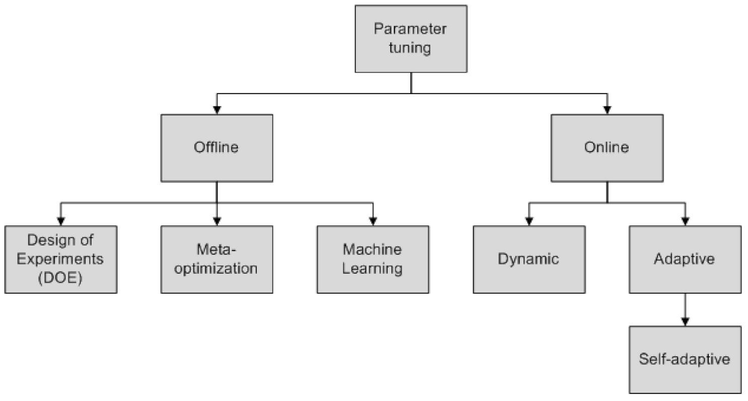
There are two different approaches to the parameter tuning of metaheuristics [15]: offline and online (Figure 1). In the offline parameter tuning, the values of various parameters are defined before the execution of the metaheuristic. On the other hand, in online approaches, parameters are controlled and updated dynamically or adaptively during the execution of the technique. These approaches are also known by parameter tuning and control, respectively [21,38,39,40,41,42].

The purpose of offline parameter tuning is to obtain parameter values that may be useful for the resolution of a large number of instances, which requires several experimental evaluations [39]. Usually, metaheuristics are tuned one parameter at a time, and their best values are empirically determined. Thus, the interaction between the parameters is generally not studied.

To overcome this problem, Design of Experiments (DOE) is often used [43,44,45]. Before being able to use a DOE approach, it is necessary to take into account the factors representing the variations of parameters and the levels representing different values for the parameters (which may be quantitative or qualitative), which means that it is a very time-consuming task [21]. Johnson [46] discussed different aspects of the DOE specification and analysis with stochastic optimization algorithms. The great disadvantage of using a DOE approach is the high computational cost when there are a large number of parameters and where the domains of the respective values are high, since a large number of experiments are need [47].

In offline parameter tuning, a meta-optimization approach can be done by any (meta)heuristic, resulting in a meta-metaheuristic [15]. Meta-optimization consists of two levels [15]: the meta-level and the base level. In the meta-level, solutions represent the parameters to optimize, such as the size of the tabu list in Tabu search, the cooling rate in simulated annealing and the crossover and mutation rates of genetic algorithms. At this level, the objective function of a solution corresponds to the best solution found (or another performance indicator) for metaheuristics with the specified parameters. Thus, each solution at the meta-level corresponds to an independent metaheuristic at the base level. Meta-optimization is largely used in evolutionary computation [48].

In problems with heterogeneous distributions, the best parameter settings can vary from instance to instance. Hutter et al. [20] demonstrated that machine learning models can make amazingly accurate predictions of runtime distributions of random and incomplete research methods such as metaheuristics, and how these models can be used to automatically adjust the parameters for each instance of a problem in order to optimize the performance, without requiring human intervention. A review on learning approaches for parameter tuning is presented in the next subsection.

Some authors argue that leaving the parameters’ values fixed during the execution of an algorithm seems to be inappropriate [21]. The idea of search algorithms that can automatically adapt their parameters during the search process has gained considerable interest among researchers [21]. They are called online approaches and monitor the progress of the searching process while adjusting the values of parameters in real time.

Online approaches can be divided into dynamic and adaptive [15,38,39]. In dynamic approaches, changes in parameter values are randomly or deterministically carried out, without taking into account the search process. In adaptive approaches, parameter values change according to the search process by memory usage or pre-established rules. A subclass, often used in the evolutionary computation community, is self-adaptive approaches consisting of the parameters’ evolutions during the search. Thus, parameters are encoded and are subject to change as different problems’ solutions [21].

3.2. Learning Approaches for Parameter Tuning

The parameter tuning of metaheuristics is still often performed without the use of automatic procedures and has received little attention from researchers. Only recently, consolidated methodologies to address this problem efficiently and effectively begun to emerge in the literature, although few fall within the application of learning approaches.

In addition to the racing algorithms (Section 3.2.1) and case-based reasoning (Section 3.2.2), described in more detail because they are used in this work to address the problem of tuning metaheuristics parameters, the reader can find other approaches in the literature. Dobslaw [49] presented a framework for simplifying and standardizing metaheuristics parameters by applying DOE and artificial neural networks. The training stage was divided into experimental and learning phases. These phases were connected and represented the greatest part of the computational time expenses. Miles-Smith [50] presented and discussed a method to solve the problem of algorithm selection, from the point of view of the learning problem, by incorporating meta-learning concepts. Stoean et al. [51] had a combined methodology to solve the parameter tuning problem in metaheuristics and used a sampling approach to generate a large diverse set of values for the parameters to be tuned. This set is then subjected to regression by use of an evolutionary approach around support vector machines. Zennaki and Ech-Cherif [52] used machine learning techniques such as decision trees, learned from a group of multiple instances of solutions randomly generated. These instances solutions are used repeatedly to predict the quality of a solution to a given instance of the combinatorial optimization problem, which is used to guide and tune the metaheuristic for more promising areas of the search space. Lessmann et al. [53] presented an approach based on data mining for dealing with the problem of tuning particle swarm optimization. The authors proposed a hybrid system employing regression models to learn appropriate values for the parameters based on past movements of this technique.

3.2.1. Racing

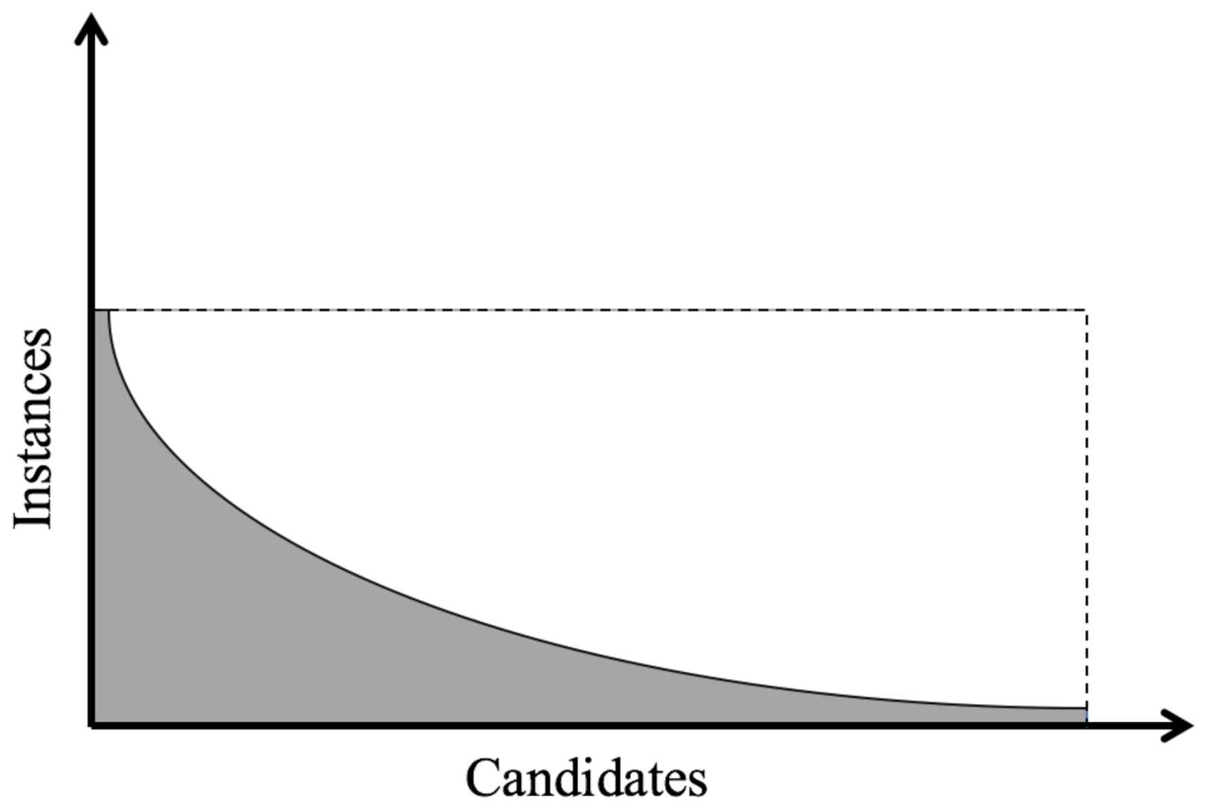
Birattari [4] argued that a brute-force approach is clearly not the best solution for solving the parameters tuning problem. A more refined and efficient way to perform metaheuristics tuning can be achieved by streamlining the evaluation of candidates and releasing those who appear to be less promising during the evaluation process. This statement summarizes the racing approaches applied to the parameters tuning of combinatorial optimization techniques (Figure 2). The information that follows is based on [4,39].

In the 1990s, Maron and Moore [54] proposed the Hoeffding race method, in order to speed up the selection of models in supervised learning problems. Hoeffding race adopted a statistical test based on the formula of Hoeffding [55], concerning the confidence in the empirical average of k positive numbers, whose sample is used independently from the same distribution.

However, the Hoeffding race adopts a non-parametric test, even if the adopted test needs knowledge of a limit on the observed error, and this aspect reduces significantly the range of applications of the method. Despite this fact, the idea behind racing approaches is very appealing. Lee and Moore [56] proposed some algorithms based on different statistical tests. Among them, BRACE is based on Bayesian statistics and implements a statistical technique known as blocking [44,57,58]. A block plan is an experimental definition that is possibly adopted when two or more candidates have to be compared. Blocks improve that comparison accuracy. A block is a set of relatively homogeneous experimental conditions under which all the candidates are tested. In the best candidate selection context, the adoption of block plans is particularly natural and simple: each survivor candidate is tested in the same examples, and each instance is therefore a block in the considered plan.

The statistical test adopted in BRACE is equivalent to the paired t-test [59] performed between each pair of survivor candidates. Contrary to the test adopted in Hoeffding race, the t-test is a parametric process and therefore is based on some assumptions concerning stochastic variables. BRACE proved to be very effective and is reported as capable of achieving better results than the Hoeffding race [54,56].

The F-race method [27] is a racing approach that integrates into a single algorithm the best features of Hoeffding race and BRACE. As already mentioned, Hoeffding race adopts a non-parametric approach but does not consider blocking. On the other hand, BRACE adopts blocking but discards the non-parametric definition by a Bayesian approach. F-race is based on the Friedman test (Friedman two-way analysis of variance by ranks) that implements a block plan in an extremely natural manner and is, at the same time, a non-parametric test [44].

To give a description of Friedman test, let us assume that F-race reached step k, where there are still $k-1$ configurations in the run. The Friedman test assumes that the observed costs for the candidates still in the race are k mutually independent random variables, called blocks. Each block corresponds to the computational results in an instance for each configuration still in the race at step k.

Birattari [4] described that, in addition to the Friedman test, the Wilcoxon test (Wilcoxon matched-pairs, signed-ranks) can be used [44] when there are only two candidates in the run, since it has proven to be more robust and efficient.

In F-race, ranking plays an important dual role. First, it is connected with the non-parametric nature of the ranking based test. The main merit of the non-parametric analysis is that it does not require the formulation of hypotheses on the distribution of observations. It is precisely in the adoption of a statistical test based on ranking that it differs from previously published works [4].

The racing approach used in this work is based on a general F-race algorithm.

3.2.2. Case-Based Reasoning

Case-based reasoning (CBR) [60] is an artificial intelligence methodology that solves new problems through the use of information about similar previous solutions. This technique has been the subject of great attention from the scientific community over the past two decades [61,62,63,64].

Previously solved problems and their solutions (or associated strategies) are stored as cases and stored in a repository, named casebase, so they can be reused in the future [65,66]. Instead of defining a set of rules or general terms, a CBR module solves the new problem by reusing previously solved similar problems [67]. Usually, it is necessary to adapt the solutions to the new case; the solutions shall be kept and the casebase updated [66]. The information described in this subsection was based on [60,61].

Case-based reasoning is a problem-solving paradigm quite different from other artificial intelligence approaches. Instead of relying only on general knowledge of a problem domain, CBR is able to use specific knowledge of previously known situations of a problem (cases). A new problem is solved by searching for a similar past case and reusing it in the new situation. Another important difference is based on the fact that CBR is an incremental and sustained approach to learning, since a new experience is retained every time a problem is solved, becoming immediate available for solving future problems.

In CBR terminology, a case usually denotes a problem situation. A previously experienced situation, which was captured and learned, is referred to as a past case. A new case that is yet unresolved is a description of a new problem to solve. Thus, CBR is a cyclical and integrated process of problem solving, learning from experience for solving new cases.

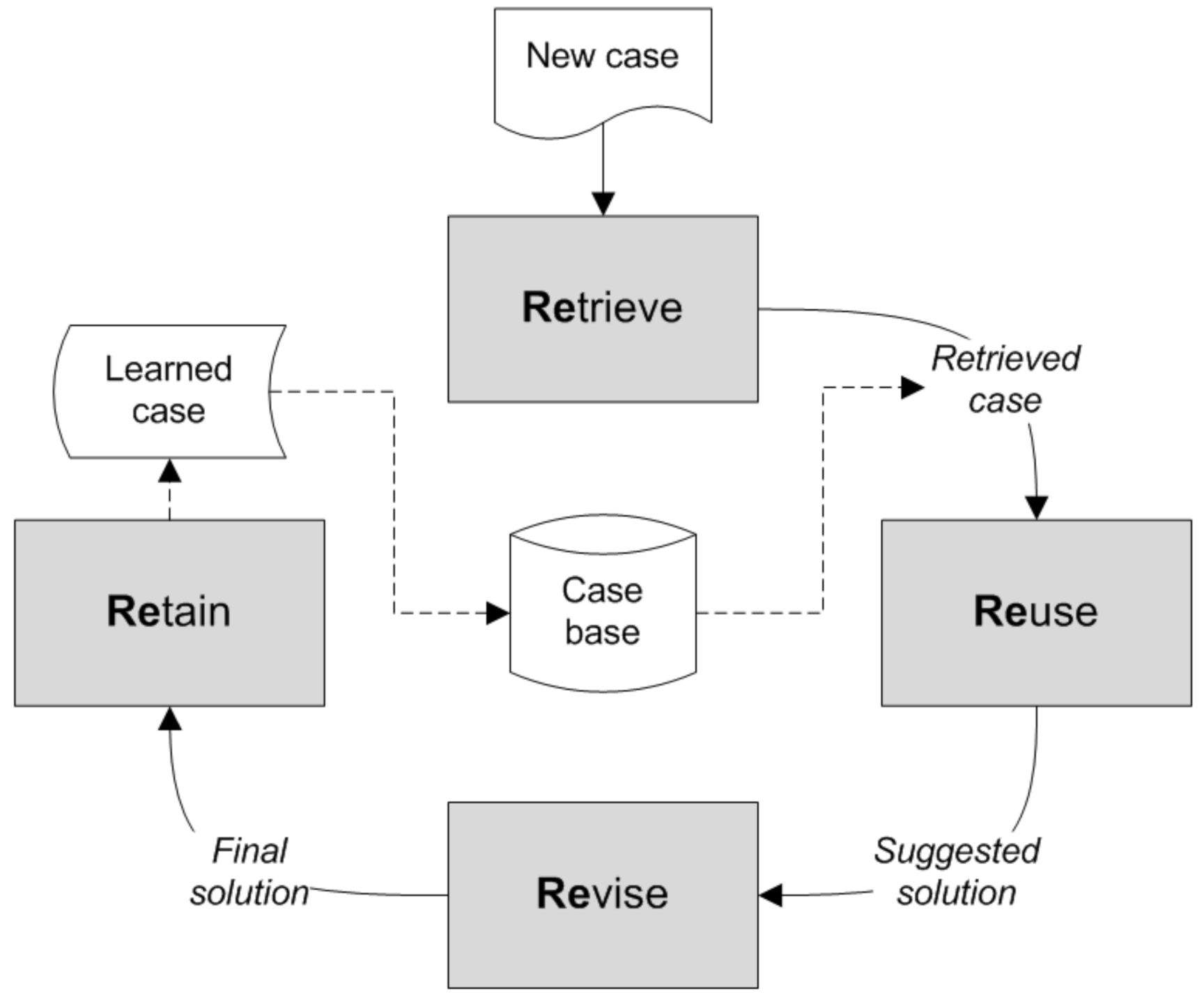
Thus, a general CBR cycle (Figure 3) can be described through the following four processes, known as “the four REs” [65,68]: retrieve the most similar case (or cases); reuse the information and knowledge from the retrieved case in order to propose a solution; revise the proposed solution; retain the newly solved case for future use.

The retrieving phase begins with a partial description of the problem and ends when the most similar case in the casebase is found. This phase requires identifying a problem, which may involve the simple observation of its features, but also more elaborate approaches in order to try to understand the problem in context, return a set of sufficiently similar cases according to a minimum similarity and select the best case among all. The reusing of the recovered case’s solution focuses on two aspects: the differences between the past and current cases; and identifying the parts of the recovered case that can be transferred to the new case, which can be accomplished through a direct copy or through some adjustments. In simpler classification tasks, the differences are considered not relevant and the recovered solution is transferred to the new case. This is a trivial kind of reusing. However, other approaches take into account the differences between the two cases, and the reused part cannot be directly transferred to the new case. It requires a process of adaptation that takes into account those differences. The revising phase’s objective is to apply the solution suggested by the reusing phase to an execution environment, evaluate the results and learn from the success (passage to the next stage) or perform solution repair through the use of a specific problem’s domain knowledge. Finally, the retention phase allows one to incorporate the useful learned knowledge in the existing knowledge. Learning from the success or failure of the proposed solution is triggered by the outcome of the evaluation and possible repair. This phase involves selecting the information to retain, in what way it should be retained, how to index the information for afuture reuse, and how to integrate the new case in the memory structure.

A new case to be solved by CBR is used to retrieve an old case from the casebase in the first stage. The aim of the second stage is to find the previous case that is the most similar to the one that was found in the casebase. This retrieved case is used to propose a solution to the new case during the reusing process. This means that, since the two cases are identical, the solution used to solve the retrieved case can also be used to solve the new case. The proposed solution is checked, for example, by implementing the method, and adapted if necessary in the revising process. Finally, in the retaining phase, the information is retained for future use, and the casebase is updated with the new learned case [60,61].

3.3. AutoDynAgents: A Multi-Agent Scheduling System

The multi-agent system for scheduling used in this work is well described in the literature and is known as AutoDynAgents [6,7,8,9].

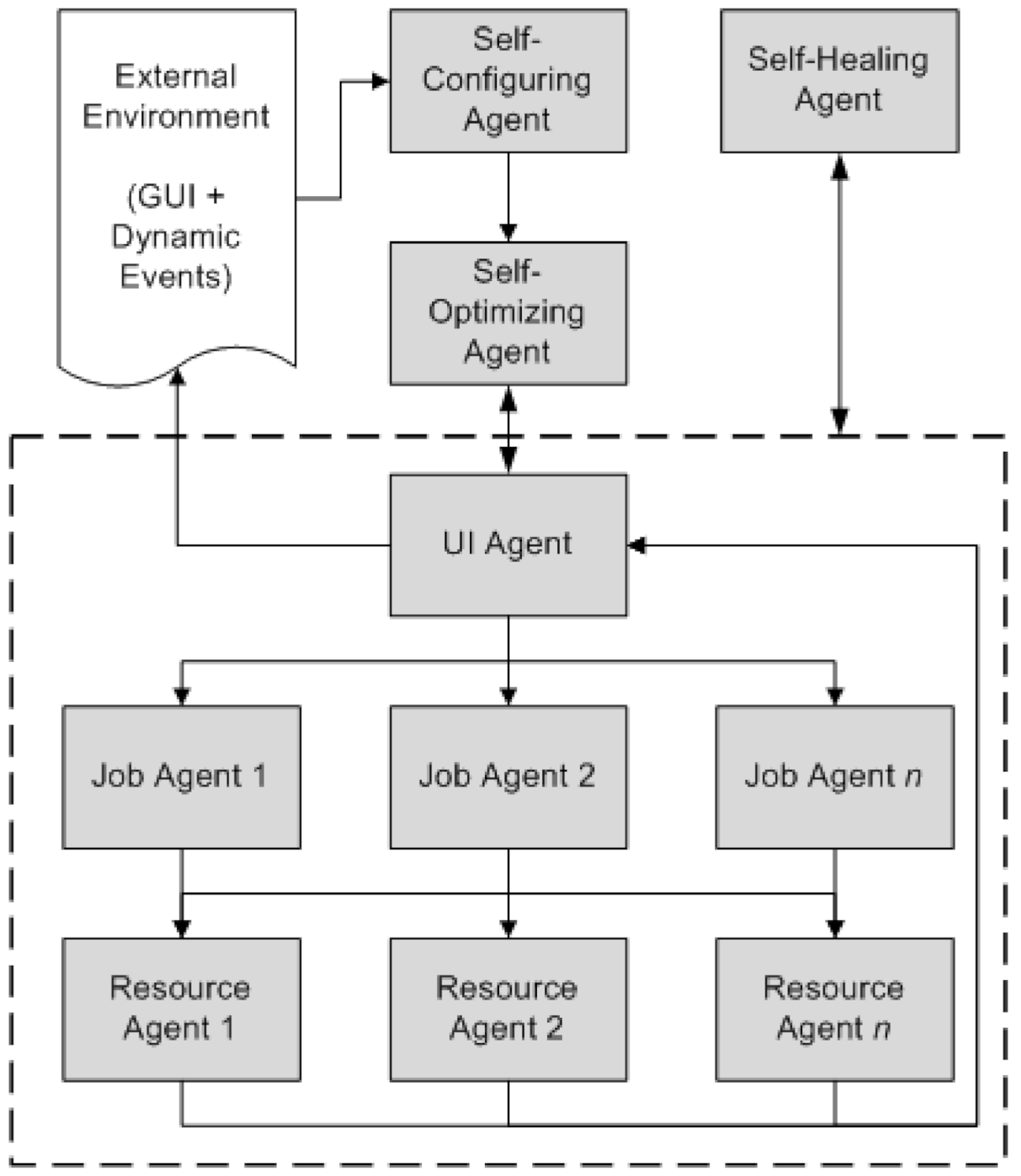
In the AutoDynAgents system (Figure 4) there are agents to represent tasks and agents representing resources (or machines). There are also agents representing some autonomic computing self-behaviors, described in [6].

In this architecture, the most important type of agent is the resource agent. Each resource agent is able to: find a (near-)optimal solution by applying a metaheuristic (Tabu search, simulated annealing, genetic algorithms, ant colony optimization, particle swarm optimization or artificial bee colony); adapt the chosen technique configuration parameters according to the problem to solve; deal with the disturbances that may occur, i.e., arrival of new tasks, canceled jobs, changing the attributes of tasks, etc.; and communicate with other agents in order to solve the given scheduling problem.

The scheduling approach used by AutoDynAgents differs from those found in the literature. Each resource agent is responsible to optimize operations for a given machine, by using metaheuristics, and then a group of agents work together to achieve a good solution to the problem, in feasible computational time.

In a generic way, the AutoDynAgents system has an autonomous architecture with a team model and consists of three main components:

• The hybrid scheduling module that uses metaheuristics and a mechanism to repair activities between resources. The purpose of this mechanism is to repair the operations executed by a machine, taking into account the tasks technological constraints (i.e., the precedence relations of operations) in order to obtain good scheduling plans.
• The dynamic adaptation module that includes mechanisms for regenerating neighborhoods/populations in dynamic environments, increasing or decreasing them according to the arrival of new tasks or cancellation of existing ones.
• The coordination module, aiming to improve the solutions found by the agents through cooperation (agents act jointly in order to enhance a common goal) or negotiation (agents compete with each other in order to improve their individual solutions).

The work on this paper focuses on the hybrid scheduling module. Specifically, the racing + CBR module is used by the self-optimizing agent. One can find more details about the dynamic adaptation module in [69,70] and about the coordination module in [13,71,72].

4. Racing + CBR Module

The goal of this work is to provide AutoDynAgents system the ability of self-parameter metaheuristic tuning, according to the scheduling instances being solved [16]. AutoDynAgents system shall be able to autonomously pick a metaheuristic and set the parameters, according to the characteristics of the current situation (e.g., size and complexity of the problem instance). In addition, the system shall be capable to switch from a technique to another, depending on the instance to treat and accumulated past experience. Regarding the AutoDynAgents system architecture, this module is inside the self-optimizing agent (Figure 4). In this proposal, the parameter tuning is done through learning based on past experience.

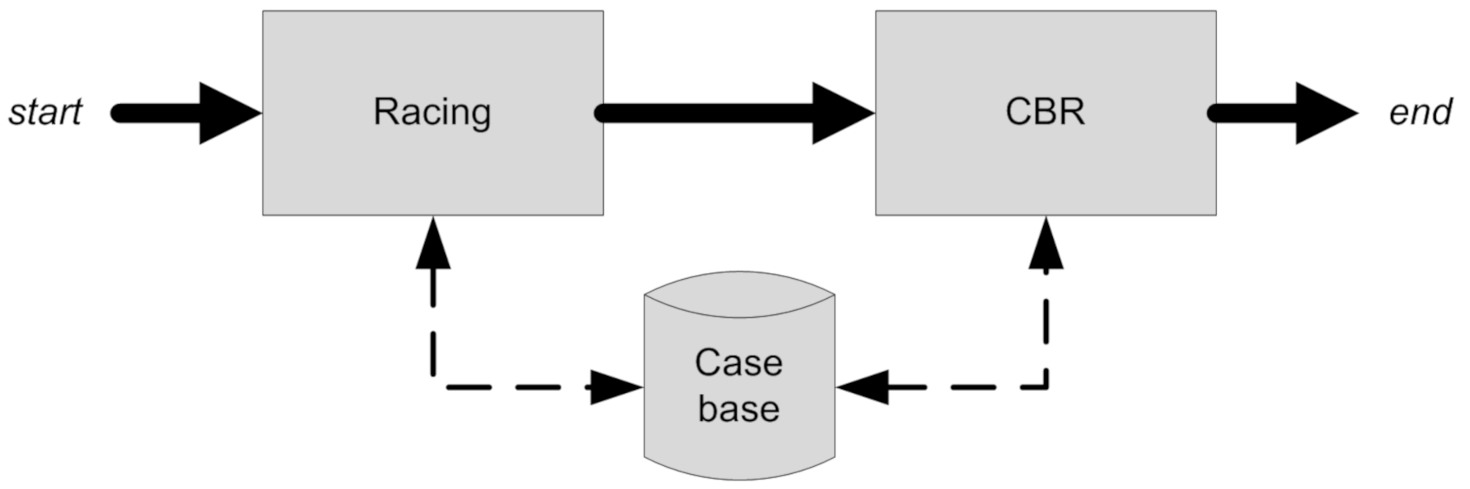
The novel proposed hybrid approach integrates two different but complementary techniques (Figure 5) [16]: racing and CBR. Racing is executed first, with the objective of an extensive study of different parameters combinations, for several instances. After finishing the racing submodule, its output acts as an input to the CBR module. The communication between the two modules is done through the casebase. For a particular instance to solve, the CBR module is responsible for the metaheuristic recommendation and tuning the respective parameters. CBR can be executed several times with the same initial racing study, and is capable of evolving during its lifetime.

4.1. Racing Submodule

The racing submodule’s goal is to carry out a study of parameter combinations for different metaheuristics, optimizing several objective functions. Algorithm 1 describes in pseudocode the steps to this study. Thus, the input parameters refer to the list of objective functions to optimize and a metaheuristics list to validate.

Algorithm 1 Racing algorithm.
Input:$listObjFunc,listMH$	▹ list of objective functions, list of metaheuristics
Begin
$listInstances\leftarrow \varnothing$	▹ array to store instances
$listParams\leftarrow \varnothing$	▹ array to store candidate parameters
$listInstances\leftarrow getInstances\left(\right)$	▹ get problem instances
for all $mh\in listMH$ do	▹ for all metaheuristics
$listParams\leftarrow getParams(objFunc,mh)$	▹ get candidate parameters
$race\leftarrow createRace\left(listParams\right)$	▹ create race to evaluate candidates
for all $instance\in listInstances$ do	▹ for all instances
for all $params\in listParams$ do	▹ for all candidate parameters
$run\leftarrow createRun(race,instance,params)$	▹ create run to evaluate each candidate parameters combination
candidate parameters combination
$executeRun\left(run\right)$
end for
$listParams\leftarrow removeCandidates(race,listParams)$	▹ remove worst candidates
end for
$best\leftarrow race.getBestCandidate\left(\right)$	▹ get the best surviving parameters combination
$race.calculateStoreAvg\left(best\right)$	▹ calculate and store the average values for the best candidate
candidate
end for
End

The first step is to get a list of candidate parameters for each metaheuristic and to make them race among each other. These races are performed for a specified number of instances. For each instance, each combination of parameters is tested in the system, and the results are stored in the database. At the end of each instance run, candidates that obtained the worst results are removed. At the end of the race, the best candidate is the one who was able to survive through all instances.

The racing submodule arises from an adaptation of the F-race method. The inability to use a direct implementation of the candidate elimination algorithm, due to lack of a sufficient number of scheduling instances, led to the need for adapting and implementing a solution where the overall operation was similar to the generic racing algorithm [4].

The most relevant part of this whole process is the removeCandidates() method, described in Algorithm 2, since it decides which candidates will be removed from the race. This algorithm takes as input parameters the current race and the list of candidate parameters, and returns the list of surviving parameters. The first check verifies if the list of candidate parameters has more than one combination; otherwise we are facing the best case. Then it needs to find out what statistical test shall be used. If the list of candidates has more than two elements, the algorithm applies the Friedman test. Otherwise, it uses the Wilcoxon test.

Algorithm 2$removeCandidates\left(\right)$ method.
Input:$race,listParams$	▹ current race, list of candidate parameters
Output:$listParams$	▹ list of surviving candidate parameters
Begin
if $size\left(listParams\right)>1$ then
$listInstances\leftarrow race.getIntances\left(\right)$	▹ gets race instances
if $size\left(listParams\right)>2$then	▹ applies Friedman when more than two
$listParams\leftarrow applyFriedmanTest(listParams,listInstances)$
else	▹ applies Wilcoxon test when there are only two candidates
$listParams\leftarrow applyWilcoxonTest(listParams,listInstances)$
end if
end if
return $listParams$
End

The Friedman test (Algorithm 3) requires that all candidates have been tested in at least two instances. This implies that at the end of the first instance, all candidates survive. Friedman test gets the ordered rankings from the candidates and calculates the sum of those rankings for each candidate. The number of survivors is the best, n (Equation (3)).

Algorithm 3 The Friedman test.
Input:$listParams,listInstances$	▹ list of candidate parameters, list of instances
Output:$listParams$	▹ list of surviving candidates
Begin
$ranks\leftarrow \varnothing$	▹ rankings matrix for candidate parameters per instance
$sumRanks\leftarrow \varnothing$	▹ array of rankings sum for candidate parameters
$inst\leftarrow size\left(listInstances\right)$	▹ number of instances
$cand\leftarrow size\left(listParams\right)$	▹ number of candidates
if $inst>1$ then
$ranks\leftarrow sortRankFriedman(listInstances,listParams)$
$sumRanks\leftarrow ranksSum\left(ranks\right)$
$surv\leftarrow calcNumSurv(inst,cand)$	▹ Equation (3)
$listParams\leftarrow getSurviving(sobrev,sumRanks)$
end if
return $listParams$
End

The number of survivors at each step (Equation (3)) is dependent on the number of instances already executed and the number of candidates. Moreover, it is calculated according to the $1/{log}_2$ function, which allows one to obtain behavior similar to the F-race. With this function, it is possible to get quick convergence to the best candidate for even a small number of instances, unlike what happens with the original F-race method.

$$\mathrm{surv}=\mathrm{round}\left(\frac{1}{{log}_2(\mathrm{inst}+1)}\times \mathrm{cand}\right)$$

(3)

where inst is the number of instances and cand is the number of candidates.

When there are only two candidates, the Wilcoxon test is used instead. The Wilcoxon test (Algorithm 4) compares two candidates slightly differently from the Friedman test. First, an array with the differences of the performance values in several instances between the first and second candidate is obtained. Next, a ranking of the absolute values of these differences is calculated, and then w values resulting from the weighted sum of the ranks and signs of difference values are calculated (Equation (4)).

$$\mathrm{w}=\sum _{\mathrm{i}=0}^{\mathrm{inst}}\mathrm{ranks}\left[\mathrm{i}\right]\times \mathrm{signs}\left[\mathrm{i}\right]$$

(4)

where inst is the number of instances, ranks[i] is the ranking of instance i and signs[i] is the signal of instance i.

Algorithm 4 The Wilcoxon test.
Input:$listParams,listInstances$	▹ list of candidate parameters, list of instances
Output:$listParams$	▹ list of surviving candidates
Begin
$inst\leftarrow size\left(listInstances\right)$	▹ number of instances
$a\leftarrow getResults(listInstances,listParams.get(0\left)\right)$	▹ array with the results per instance for the first candidate
$b\leftarrow getResults(listInstances,listParams.get(1\left)\right)$	▹ array with the results per instance for the second candidate
$dif\leftarrow calcDifference(a,b)$	▹ array with the difference between the first and second candidates
$absDif\leftarrow abs\left(dif\right)$	▹ array with the absolute value for the differences
$ranks\leftarrow calcRankings\left(absDif\right)$	▹ array with the rankings of the differences
$signs\leftarrow calcSign\left(dif\right)$	▹ array with the signal of the differences
$w\leftarrow calcW(ranks,signs,inst)$	▹ value to validate the Wilcoxon test, calculated by Equation (4)
if $w<0$ then
$listParams.remove\left(1\right)$	▹ first candidate is better, remove the second
else
$listParams.remove\left(1\right)$	▹ second candidate is better, remove the first
end if
return $listParams$
End

If the w value is less than zero, it means that the first candidate is better; otherwise, the second candidate is chosen. In any case, the worst candidate is eliminated.

4.2. CBR Submodule

The CBR submodule’s aim is to find the most similar case with the new problem, regardless of which metaheuristic is used. As a consequence, the returned case includes the metaheuristic and the necessary parameters to use. Since the device must determine which procedure and parameters to use, this method seems to be appropriate for the problem at hand.

The CBR submodule consists of a cycle similar to that described in Section 3.2.2. This cycle consists of four main processes: retrieve, reuse, revise and retain (see Algorithm 5). Note that, in the revise stage, there is communication with the multi-agent system in order to execute the new case and extract results of completion and execution times.

Algorithm 5 Case-based reasoning
Input:$newCase$
Begin
$listCases\leftarrow retrieve\left(newCase\right)$	▹ retrieving phase
$bestCase\leftarrow reuse\left(listCases\right)$	▹ reusing phase
$solution\leftarrow getSolution\left(bestCase\right)$	▹ get the solution for the best case
$simBestCase\leftarrow getSimilarity\left(bestCase\right)$	▹ get the similarity
$revisedSolution\leftarrow revise(solution,simBestCase)$	▹ revising phase
$results\leftarrow executeCaseMAS(newCase,revisedSolution)$	▹ execute in MAS
$retain(newCase,revisedSolution,results)$	▹ retaining phase
End

Whenever a new instance arises, the CBR submodule creates a new case, which is solved through the recovery of one or more previous similar cases. After obtaining a list with the most similar cases, the most similar case among all is reused and is suggested as a possible solution. In the next step, and before proceeding to the communication with the multi-agent system, the revision of the suggested solution is performed by adjusting and refining the parameters. Finally, the case is accepted as a final solution and retained in the case base as a new learned case.

4.2.1. Retrieving Phase

The retrieving phase aims to search the casebase for the most similar past cases with the new case, and retrieve them for analysis in order to be subsequently selected one of the best cases and reuse it in the next phase.

This phase, described in Algorithm 6, receives the new case as an input parameter. As output parameter, the algorithm returns a list of retrieved cases; each list element is a case-similarity pair where each case and the respective similarity with the new case are specified.

Algorithm 6 Retrieving phase.
Input:$newCase$
Output:$listCases$	▹ list of retrieved cases, with similarities
Begin
$listCases\leftarrow \varnothing$
$minSim\leftarrow 0.70$	▹ minimum similarity
$listPreCases\leftarrow queryCaseBase\left(newCase\right)$	▹ pre-select the casebase
for all$case\in listPreCases$ do
$sim\leftarrow calcSimilarity(case,newCase)$	▹ calculate the similarity
if $sim\ge minSim$then	▹ if similarity greater than minimum similarity
$listCases.add(case,sim)$	▹ add case to list
end if
end for
return $listCases$
End

A minimum similarity of 0.70 in a $[0,1]$ range was defined, which means a case needs to be at least 70% similar to the new case to be selected. This minimum similarity is the sum of $Njobs$, $ProbType$ and $MultiLevel$ weights, explained further in the Equation (6).

After initializing the variables, the algorithm begins by making a pre-selection of cases, to select only cases that might be considered sufficiently similar, i.e., with similarity greater than the minimum similarity of 0.70.

For each pre-selected case, the similarity to the new case is calculated, and if it is better than or equal to the previously specified minimum similarity, the case is added to the list to be returned, together with the respective similarity value. At the end of the algorithm, this list of cases is returned.

One of the most important aspects of a CBR system is the similarity measure between cases. The attributes to consider for the similarity measure are: the number of tasks ($Njobs$), the number of machines ($Nmachines$), the type of problem ($ProbType$), the multi-level (if instances have operations with more than one precedence) feature ($MultiLevel$) and the known optimal conclusion time ($Opt{C}_{max}$). These attributes are weighted differently in the similarity measure, as defined in Equation (5). The similarity measure is a value between zero (0) and one (1), corresponding to no similar cases and equal cases respectively. It is the result of a weighted sum of the similarities between the different attributes.

In Equation (6), the weights for each attribute are presented. More importance is given to $Njobs$ and $Nmachines$, as these are the ones that best define the problem dimension, a fundamental characteristic for metaheuristic tuning. $Njobs$ is the most important attribute of the problem dimension, since it defines how many jobs are processed. $Nmachines$ defines how these tasks are divided for processing. Thus, we considered a weight of 50% for $Njobs$ and 25% for $Nmachines$. These two attributes together represent 75% of the similarity measure. $ProbType$, with 15%, represents some importance for the parameter tuning, since, e.g., a job–shop problem introduces additional complexity as compared to a single machine problem. With only 5% each, it was considered that $MultiLevel$ and $Opt{C}_{max}$ are not as important as other attributes; however, they are important for the verification of very similar cases. The $Opt{C}_{max}$ attribute was taken into account in order to make it possible to know whether the new case has been previously processed or not because, when known, this is a unique characteristic of a problem.

$$\mathrm{similarity}=\sum _{\mathrm{i}=0}^{\mathrm{n}}{\mathrm{w}}_{\mathrm{i}}\times {\mathrm{sim}}_{\mathrm{i}}$$

(5)

where ${\mathrm{w}}_{\mathrm{i}}$ is the weight of characteristic i and ${\mathrm{sim}}_{\mathrm{i}}$ is the similarity of characteristic i.

$$\begin{array}{c}\hfill {\mathrm{w}}_{\mathrm{Njobs}}=0.50;{\mathrm{w}}_{\mathrm{Nmachines}}=0.25;{\mathrm{w}}_{\mathrm{ProbType}}=0.15;{\mathrm{w}}_{\mathrm{MultiLevel}}={\mathrm{w}}_{{\mathrm{OptC}}_{\max }}=0.05;\end{array}$$

(6)

$${\mathrm{sim}}_{\mathrm{Njobs}}=\frac{min({\mathrm{Njobs}}_1,{\mathrm{Njobs}}_2)}{max({\mathrm{Njobs}}_1,{\mathrm{Njobs}}_2)}$$

(7)

$${\mathrm{sim}}_{\mathrm{Nmachines}}=\frac{min({\mathrm{Nmachines}}_1,{\mathrm{Nmachines}}_2)}{max({\mathrm{Nmachines}}_1,{\mathrm{Nmachines}}_2)}$$

(8)

$${\mathrm{sim}}_{\mathrm{ProbType}}=\left\{\begin{array}{cc}0\hfill & \mathrm{if}{\mathrm{ProbType}}_1\ne {\mathrm{ProbType}}_2\hfill \\ 1\hfill & \mathrm{if}{\mathrm{ProbType}}_1={\mathrm{ProbType}}_2\hfill \end{array}\right.$$

(9)

$${\mathrm{sim}}_{\mathrm{MultiLevel}}=\left\{\begin{array}{cc}0\hfill & \mathrm{if}{\mathrm{MultiLevel}}_1\ne {\mathrm{MultiLevel}}_2\hfill \\ 1\hfill & \mathrm{if}{\mathrm{MultiLevel}}_1={\mathrm{MultiLevel}}_2\hfill \end{array}\right.$$

(10)

$${\mathrm{sim}}_{{\mathrm{OptC}}_{\max }}=\left\{\begin{array}{cc}\frac{\min ({\mathrm{OptCmax}}_1,{\mathrm{OptCmax}}_2)}{\max ({\mathrm{OptCmax}}_1,{\mathrm{OptCmax}}_2)}\hfill & \mathrm{if}{\mathrm{OptCmax}}_1\ge 0\mathrm{and}{\mathrm{OptCmax}}_2\ge 0\hfill \\ 0\hfill & \mathrm{if}{\mathrm{OptCmax}}_1<0\mathrm{or}{\mathrm{OptCmax}}_2<0\hfill \end{array}\right.$$

(11)

The Njobs and Nmachines similarities (Equations (7) and (8)) are calculated in the same way, yielding a value in a $[0;1]$ range. The ProbType and MultiLevel similarities (Equations (9) and (10)) can be one (1) if they are the same, or zero (0) if they are different. For ${\mathrm{OptC}}_{\max }$ (Equation (11)) the similarity is calculated identically to Njobs and Nmachines if the values of the two cases are positive. If any value is less than zero (0), this means that the value is not known, and in this case the similarity for ${\mathrm{OptC}}_{\max }$ is zero.

4.2.2. Reusing Phase

In the reusing phase, the most similar case to the new case is selected, and the respective solution is suggested as a possible solution. Thus, the metaheuristic and the parameters used for the resolution of that case are copied to the resolution of the new case.

In Algorithm 7, three variables are initialized: $simVerySimilar$ to determine if two cases are very similar; $listBestCases$ for storing the list of best retrieved cases; and $minRatio$ to serve as a comparison determining the best cases.

Algorithm 7 Reusing phase.
Input:$listCases$
Output:$bestCase$
Begin
$simVerySimilar\leftarrow 0.95$	▹ similarity to validate if two cases are very similar
$minRatio\leftarrow 0.75$	▹ minimum ratio to add a case into $listBestCases$
$listBestCases\leftarrow \varnothing$	▹ list to store the best cases
if listCases is empty then
$bestCase\leftarrow applyPreDefinedParameters\left(\right)$
else
for all $case\in listCases$ do
if $compareSims(case,bestCase)\ge simVerySimilar$ then
$ratio\leftarrow case.OptCmax/case.Cmax$
if $ratio\ge minRatio$ then
$listBestCases.add\left(case\right)$
else
$ratioBest\leftarrow bestCase.OptCmax/bestCase.Cmax$
if $ratio=ratioBest$ then
if $case.TimeExec<bestCase.TimeExec$ then
$bestCase\leftarrow case$
end if
else	▹ cases are not very similar, so compare similarities directly
if $ratio>ratioBest$then	▹ case is more effective
$bestCase\leftarrow case$	▹ update best case
end if
end if
end if
else	▹ cases are not very similar, so compare similarities directly
if $case.Sim>bestCase.Sim$then	▹ case more similar
$bestCase\leftarrow case$	▹ update best case
end if
end if
if listBestCases is not empty then
$index\leftarrow random(0,size(listBestCases\left)\right)$	▹ randomly selects a case to be considered as the best
$bestCase\leftarrow listBestCases.get\left(index\right)$
end if
end for
end if
return$bestCase$
End

First, the algorithm checks if the list of retrieved cases is not empty. If it is empty, then there are no cases with similarity higher than the minimum similarity. This means that the predefined parameters are used, working as a starting point for the resolution of future similar cases.

When the list of retrieved cases has elements, the most effective cases are selected. However, if there is no effective case, the most similar case is selected. In this cycle, some checks are carried out to determine if there are cases with very high similarity. If so, the best cases or the most effective/efficient cases are selected, by comparing the conclusions and running times. The verification of very similar cases is performed using Equation (12), and then the value is compared with $simVerySimilar$. For this variable, the value of 0.95 was considered; two cases are very similar if the ratio of their similarities is greater than 95%.

When there are very similar cases, it is necessary to calculate the ratio (Equation (13)) between $OptCmax$ and $Cmax$ of each case to make the comparison with $minRatio$. This variable indicates that a case is considered as one of the best if the ratio of its $OptCmax$ by its $Cmax$ is equal to or greater than 75%. When this happens, the case is added to $listBestCases$.

When the ratio of a case, $rati{o}_{case}$, is not greater than $minRatio$, it is necessary to calculate the ratio for the best case so far. If the ratio of a particular case is equal to $bestCase$ ratio, the two cases are equally effective and it is necessary to compare the execution times. If the case runtime is lower than $bestCase$, then $bestCase$ is updated as a more efficient case has been found. The $bestCase$ is also updated if the ratio of a particular case is higher than $bestCase$ ratio, as a more effective case has been found.

When there are not very similar cases, the best case is chosen by a direct comparison between the similarities from the list of cases.

In the end, if $listBestCases$ is not empty, one of best cases is randomly selected, thereby ensuring that $bestCase$ is one of the top cases and not simply the best among all. This proves to be important to avoid stagnation and to avoid choosing the same case too often, which would not allow the evolution of the system. If the best case among all is always selected, whenever a new similar case appears, the same case will be selected, except if the new cases always obtain better results, which is not true due to the underlying stochastic component of metaheuristics.

If $listBestCases$ is empty, the best case is the most similar one or it is the case that has the best effectiveness-efficiency value.

$$\mathrm{CompareSims}({\mathrm{case}}_1,{\mathrm{case}}_2)=\frac{min({\mathrm{sim}}_{{\mathrm{case}}_1},{\mathrm{sim}}_{{\mathrm{case}}_2})}{max({\mathrm{sim}}_{{\mathrm{case}}_1},{\mathrm{sim}}_{{\mathrm{case}}_2})}$$

(12)

where ${\mathrm{sim}}_{{\mathrm{case}}_{\mathrm{n}}}$ is the similarity of ${\mathrm{case}}_{\mathrm{n}}$ to the new case.

$${\mathrm{ratio}}_{\mathrm{case}}=\frac{{\mathrm{OptCmax}}_{\mathrm{case}}}{{\mathrm{Cmax}}_{\mathrm{case}}}$$

(13)

where ${\mathrm{OptCmax}}_{\mathrm{case}}$ is the optimum completion time for case and ${\mathrm{Cmax}}_{\mathrm{case}}$ is the obtained completion time.

$$\mathrm{credit}=10+(1-\mathrm{simCredMin})\times 100$$

(14)

$$\mathrm{credit}=10+(1-\mathrm{simBestCase})\times 100$$

(15)

4.2.3. Revising Phase

On the revising phase (Algorithm 8), the CBR submodule proceeds with an adaptation of the solution suggested by the Reusing phase. The direct use of the suggested solutions can lead to system stagnation, and thus can leave the system unable to evolve for better results. Thus, to escape from local optimal solutions and system stagnation, this algorithm applies some diversity (disturbance) to the solutions.

Algorithm 8 Revising phase.
Input:$solution,simBestCase$
Output:$revisedSolution$
Begin
$revisedSolution\leftarrow \varnothing$
$simCredMin\leftarrow 0.95$
$credit\leftarrow 0$
if $simCredMin<simBestCase$ then
$credit=10+(1-simCredMin)\times 100$
else
$credit=10+(1-simBestCase)\times 100$
end if
$creditsArray\leftarrow returnCredits(credit,solution)$	▹ calculate perturbation
$revisedSolution\leftarrow solution.updateParameters\left(creditsArray\right)$
return $revisedSolution$
End

Algorithm 8 takes two input parameters, namely, the solution suggested by the reusing phase (i.e., the suggested metaheuristic and respective parameters) and the best case similarity. The algorithm returns the same metaheuristic with the revised and changed parameters. Two important variables are used: $credit$ representing the overall credit to be distributed by the parameters; and $simCredMin$ representing an auxiliary variable to ensure a minimal credit. The latter is initialized with the value 0.95, which is the maximum similarity for which the credit is inversely proportional. This means that cases with similarity greater than 95% have the same overall credit to be applied in the inclusion of disturbance.

The second task performed by the algorithm is to verify if the similarity of the most similar case is greater than 95%. If so, then the credit is initialized with the minimum value of 15, depending on the value of $simCredMin$ variable (Equation (14)). Otherwise, the credit will be inversely proportional to the similarity of the best case (Equation (15)). This means that the less similar a case is, the more disturbance there will be in the parameters of the suggested metaheuristic.

After initializing the credit, the $returnCredits\left(\right)$ method is called to distribute the credit through the different parameters (Algorithm 9). After distributing the credit among the parameters, the next step is to update the parameters’ values. The $returnCredits\left(\right)$ algorithm takes two parameters, the global credit and the metaheuristic with the parameters to update, and returns an array with the credits to be used in each parameter.

Algorithm 9$returnCredits\left(\right)$ method.
Input:$credit,solution$
Output:$creditsArray$
Begin
$creditsArray\leftarrow \varnothing$
for all $param\in solution.listParams$ do	▹ for all parameters
if $credit>0$ then
$creditsArray\left[param\right]\leftarrow random(0,credit/2)$	▹ random credit
$credit=credit-creditsArray\left[param\right]$	▹ discount given credit
if $random(0,1)=1$then	▹ decide sign of the value
$creditsArray\left[param\right]\leftarrow -creditsArray\left[param\right]$	▹ negative if true
end if
else
$creditsArray\left[param\right]\leftarrow 0$	▹ there is no more credit to give
end if
end for
return $creditsArray$
End

Assigning credit to parameters is only possible if there is enough global credit available, so that is the first check to make. If there is enough credit then the value assigned to a parameter is a random value in the range $[0;credit/2]$, uniformly distributed. This value is stored in an array and discounted from the global credit. Then a random calculation to decide whether the disturbance will be added or removed to the parameter is made. Thus, if the value is “true” (1), the credit parameter is set to a negative value, resulting in a decrease in the value of the parameter; otherwise, it is an increase. In the end, the array of parameter credits is returned.

In Equation (16), the formula for updating the parameters values is presented. For integer numbers, units are rounded. For float values, the rounding is done to the second decimal place. The reader should note that, if the credit of the parameter has a negative value, this will result in a decrease, as previously explained.

With this procedure, the system is capable of introducing disturbances in the suggested solutions and also escaping the stagnation to achieve better results.

$$\mathrm{param}=\mathrm{param}+\mathrm{round}\left(\left(\mathrm{param}\times \frac{\mathrm{creditsArray}\left[\mathrm{param}\right]}{100}\right),\mathrm{d}\right)$$

(16)

where param is the parameter that is being updated and d assumes the number of decimal places with which to perform the rounding (i.e., 0 or 2).

4.2.4. Retaining Phase

Finally, after executing the new case, it is necessary to store the information in the casebase, which is performed in the retaining phase. First, values of conclusion and execution times are collected, resulting from the execution of the new case in the multi-agent system. The solution is retained for future use. With this phase, the CBR cycle is concluded. In the next run, this newly solved case will be available to be used in the resolution of a new case.

5. Computational Results and Discussion

This section presents and describes the computational experiments for the validation of the proposed racing + CBR approach. Benchmark instances of job–shop scheduling problems extracted from OR-Library (http://people.brunel.ac.uk/~mastjjb/jeb/info.html, accessed on 7 February 2021) have been used. The reader shall note that the proposed hybrid approach is compared separately with each of the techniques used, racing and CBR, but racing + CBR is also compared with previously published results (a previous approach: [9]).

The implementation was performed via Java programming language, using a H2 database and Hibernate framework as the database access layer. The computer used for the computational study was an HP Z400 with the following key features: Intel Xeon W3565 3.20 GHz processor, 6GB DDR3 RAM memory, Samsung HD103SJ 1TB 7200rpm hard drive and Microsoft Windows 7 operating system.

Both of the outcomes are consistent with the goal of reducing the completion time ($C_{max}$). Every instance was run five times, with the average of the results determined. The ratio between the optimum value and the average value of $C_{max}$ was used to normalize the values (Equation (17)) to estimate the deviation value obtained from the value of the optimal solution cited in the literature.

$$\mathrm{ratio}=1-\frac{{\mathrm{OptC}}_{\max }}{{\mathrm{C}}_{\max }}$$

(17)

where ${\mathrm{OptC}}_{\max }$ is the optimum completion time and ${\mathrm{C}}_{\max }$ is the obtained completion time.

Rather than comparing the values directly, the deviations of the average values of ${\mathrm{C}}_{\max }$ from the optimum value are compared, which is especially useful when dealing with different ${\mathrm{C}}_{\max }$ values. Considering, for instance, two scenarios where the optimum values are 60 and 90, respectively, if we get 65 for the first instance and 98 for the second, we can infer that the value obtained for the second instance is closer to the optimum, since the ratio is 0.103 for the first and it is 0.082 for the second.

The CBR casebase was initialized based on the parameters obtained by the racing module. These parameters are shown in

Table 1. Values of Tabu search parameters. n is the number of tasks. $NeighGen$ is the percentage of generated neighbors. $NeighSize$ is the size of the neighborhood. $TabuListLen$ is the length of the tabu list.

MH	n	$\mathbf{NeighGen}$	$\mathbf{NeighSize}$	$\mathbf{TabuListLen}$	Stopping Criteria
TS	10			3	50
	15			1
	20	15%	100%	2	125
	30			3	175
	50			5	200

,

Table 2. Values of genetic algorithm parameters. $InitPopGen$ is the percentage of the initial population. $PopSize$ is the size of the population. $NumGen$ is the number of generations. $CrossRate$ is the crossover rate. $MutRate$ is the mutation rate.

MH	n	$\mathbf{InitPopGen}$	$\mathbf{PopSize}$	$\mathbf{NumGen}$	$\mathbf{CrossRate}$	$\mathbf{MutRate}$
GA	10			100	75%	1%
	15		100%	125	65%
	20	15%		150
	30			200	75%
	50		35%	400

,

Table 3. Values of simulated annealing parameters. $InitTemp$ is the initial temperature. $\alpha$ is the cooling factor. $NumItK$ is the number of iterations at the same temperature.

MH	n	$\mathbf{InitTemp}$	$\mathit{\alpha }$	$\mathbf{NumItK}$	Stopping Criteria
SA	10			5	30
	15			10	70
	20	15%	80%	20
	30			30	90
	50				200

,

Table 4. Values of ant colony optimization parameters. $Ants$ is the number of ants. $EvapRate$ is the pheromone evaporation rate. $\alpha$ controls the influence of pheromones. $\beta$ controls the desirability of state transitions.

MH	n	$\mathbf{Ants}$	$\mathbf{EvapRate}$	$\mathit{\alpha }$	$\mathit{\beta }$	Stopping Criteria
ACO	10	20		2	2	75
	15	50			1	100
	20	30	80%	1	2
	30	50		2		250
	50	75			1	350

,

Table 5. Values of particle swarm optimization parameters. $Part$ is the number of particles. $mIn$ is the minimum inertia. $MIn$ is the maximum inertia. $c1$ and $c2$ are learning factors. $mVel$ is the minimum velocity. $MVel$ is the maximum velocity.

MH	n	$\mathbf{Part}$	Stopping Criteria	$\mathbf{mIn}$	$\mathbf{MIn}$	$\mathit{c}1$	$\mathit{c}2$	$\mathbf{mVel}$	$\mathbf{MVel}$
PSO	10	30	1000
	15	25	1500
	20		1750	40%	95%	2	2	−4	4
	30	75	3500
	50		4500

and

Table 6. Values of artificial bee colony parameters. $Sn$ is the size of the population. $MaxFail$ is the maximum failures allowed.

MH	n	$\mathbf{Sn}$	$\mathbf{MaxFail}$	Stopping Criteria
ABC	10	75	1250	2000
	15		1750	3000
	20		2000	3500
	30	125	2250	4000
	50			4500

and correspond to the outputs from the racing module. In this hybrid approach, 150 initial cases were inserted, corresponding to the tuning of six metaheuristics in 25 instances.

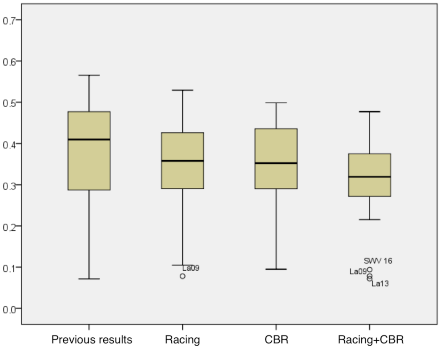
The analysis of the CBR module was carried out using the initial casebase filled by racing, with the system being run in test instances. The descriptive analysis of the ratio of the average $C_{max}$ for all approaches, including racing + CBR, is presented in

Table 7. Descriptive analysis of the $C_{max}$ ratio for all approaches, including the obtained minimum values, maximum values, averages and standard deviations.

	Min Value	Max Value	Average	$\mathit{\sigma }$
Previous results	0.07	0.57	0.3792	0.13217
Racing	0.08	0.53	0.3474	0.11834
CBR	0.09	0.50	0.3388	0.10736
Racing + CBR	0.07	0.48	0.3142	0.10999

. By examining the chart in Figure 6, analyzing the median and dispersion of data, it is possible to draw conclusions about the benefits of the racing + CBR method.

When comparing the results of the racing + CBR approach to the results of the racing module, one can see a slight improvement in the results, especially in the dispersion, indicating that the addition of the CBR module can keep the results more consistent.

In Table 7, it is possible to conclude for a lower average and standard deviation than the racing module, and lower maximum and minimum values, which is crucial given that the scheduling problem is a minimization problem.

When comparing the findings of the hybrid approach to those of CBR, the difference is not as important, indicating that combining the two modules could be beneficial. In Table 7, the minimum and maximum values have improved, as has the average, but the standard deviation has increased marginally, though the difference is not important.

Finally, the results of the racing + CBR are compared with the previous published results [9]. At this point, clear improvements are shown, which indicates a statistically significant advantage in using learning algorithms in the tuning of metaheuristic parameters in optimization problems. In Table 7 it is possible to note significant improvements, especially in the average and standard deviation. The minimum values were equal, but our maximum was lower.

Analyzing the statistical significance of these findings becomes critical at this stage. When comparing the previous published results and the results of the hybrid approach (

Table 8. Student’s t test for paired samples.

	Average	$\mathit{\sigma }$	t	DoF	p
Previous vs. Racing + CBR	0.06496	0.06499	5.475	29	0.000
Racing vs. Racing + CBR	0.03314	0.03582	5.068	29	0.000
CBR vs. Racing + CBR	0.02454	0.05208	2.581	29	0.015

), one can claim, with a 95% confidence level, that there are statistically significant differences between the results obtained initially (without learning) and the results obtained by the racing + CBR approach, allowing one to infer as to the benefit of its use. The same conclusions are possible to find about the comparison of the hybrid method against the results of racing and CBR approaches separately.

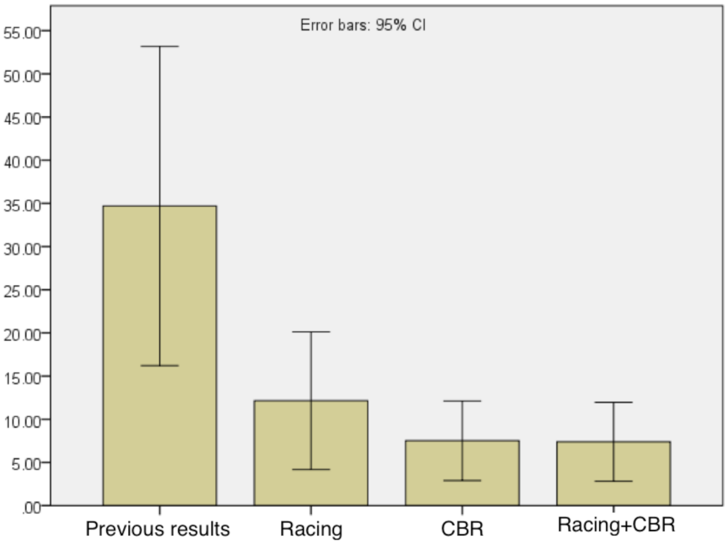
To complete the study, in Figure 7 the average execution times achieved by AutoDynAgents system with the inclusion of the racing + CBR approach are presented. By comparing the average execution times of all approaches, it is possible to show that the hybrid approach significantly improved compared to previous published results, and also there was a slight improvement in the racing based approach. However, there is no evidence of improvements in efficiency compared to CBR. Thus, in addition to improving the effectiveness of the results, the racing + CBR approach also allowed us to improve system efficiency, especially when compared to the previous results (without learning).

A total of 30 instances from OR-Library were considered and solved using each of the four approaches: previous; CBR; racing; racing + CBR. Therefore, four paired samples of 30 observations each were obtained. The results were normalized. The statistical analysis was conducted using R [73].

Table 9. Median, mean, standard deviation and Shapiro–Wilks’ normality test p-values for the results obtained with the four approaches.

Approach	Median	Mean	Std. Deviation	Shapiro Wilks’ p-Value
Previous	$0.4095$	$0.3792$	$0.1321693$	$0.10$
CBR	$0.35210$	$0.33880$	$0.107356$	$0.11$
Racing	$0.35770$	$0.34740$	$0.1183369$	$0.08$
Racing + CBR	$0.31900$	$0.31420$	$0.1099901$	$0.06$

shows that there are differences between “previous” and all the other approaches for the set of tested instances. The p-values obtained for both the Friedman-aligned ranks and Quade tests indicate very strong evidence against the null hypothesis that the results using previous results and the other three approaches have the same median (see

Table 10. Multiple comparisons test results.

	Test Statistics	Df	p-Value
Friedman’s Aligned Rank	$37.939$	3	$2.911\times {10}^{-8}<0.05$
Quade	$16.988$	3	$9.052\times {10}^{-9}<0.05$

) for solving job–shop scheduling problems. Therefore, there are at least two solution sets that have different medians of the results.

The results from comparing the racing, CBR and racing + CBR approaches against previous results, which acts as a control group, are shown in

Table 11. Post hoc tests using previous as a control group.

	CBR	Racing	Racing + CBR
p-value	$7.22\times {10}^{-6}<0.05$	$0.0018<0.05$	$5.95\times {10}^{-12}<0.05$

. Since all the p-values are <0.05, we may conclude that there are significant differences between all the approaches and the control.

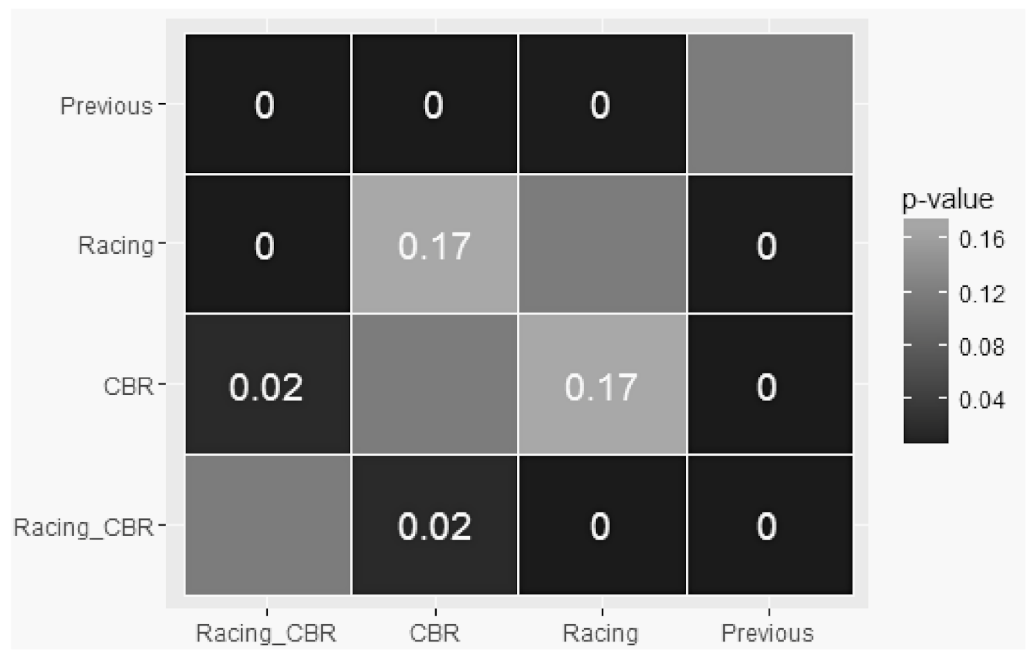
The results for all pair-wise comparison are depicted in

Table 12. Post hoc tests for all pair-wise comparisons.

	CBR	Racing	Racing + CBR
Previous	$2.2\times {10}^{-5}<0.05$	$3.6\times {10}^{-3}<0.05$	$3.6\times {10}^{-11}<0.05$
CBR		$1.7\times {10}^{-1}>0.05$	$1.7\times {10}^{-2}<0.05$
Racing			$5.1\times {10}^{-4}<0.05$

and Figure 8. We can see that, for a 5% significance level, there are significant differences between: (i) previous and all the other approaches; (ii) CBR and racing + CBR; (iii) racing and racing + CBR.

Since for each sample the normality was not rejected (see Table 9), for the pairwise comparison, the paired-sample t-test was used. The results depicted in

Table 13. Results for the paired-wise comparison.

Null Hypothesis	Alternative Hypothesis	p-Value
${\eta }_{Previous}={\eta }_{CBR}$	${\eta }_{Previous}>{\eta }_{CBR}$	$0.0002214<0.05$
${\eta }_{Previous}={\eta }_{Racing}$	${\eta }_{Previous}>{\eta }_{Racing}$	$2.611\times {10}^{-5}<0.05$
${\eta }_{Previous}={\eta }_{Racing+CBR}$	${\eta }_{Previous}>{\eta }_{Racing+CBR}$	$3.392\times {10}^{-6}<0.05$
${\eta }_{CBR}={\eta }_{Racing+CBR}$	${\eta }_{CBR}>{\eta }_{Racing+CBR}$	$0.007589<0.05$
${\eta }_{Racing}={\eta }_{Racing+CBR}$	${\eta }_{Racing}>{\eta }_{Racing+CBR}$	$1.05\times {10}^{-5}<0.05$

shows, at a 5% significance level, that ${\eta }_{Previous}>{\eta }_{CBR}>{\eta }_{Racing+CBR}$ and ${\eta }_{Previous}>{\eta }_{Racing}>{\eta }_{Racing+CBR}$.

In conclusion, there is evidence, with 95% certainty, that:

• The median results using previous are larger than the medians of the results obtained from CBR; racing; racing + CBR. Therefore all of the approaches CBR, racing and racing + CBR present improvements when compared to “previous”.
• There are no significant differences between CBR and racing, so using one of those techniques improves the results obtained with previous, but there are no differences between the performances of CBR and racing approaches.
• Combining CBR and racing into a new approach racing + CBR improves the results when compared to using previous or CBR or racing.

6. Conclusions

In the field of scheduling problems, this paper suggested a novel hybrid learning method for parameter tuning metaheuristics.

Since parameter tuning is so critical in the process of developing and implementing optimization techniques, the proposed hybrid approach was based on racing and CBR, with the goal of performing metaheuristic selection and tuning. While racing is used to assess a group of applicants in a refined and efficient manner, releasing those that tend to be less promising during the selection process, CBR uses previous similar cases to solve new cases, allowing for learning from experience. The metaheuristics used to generate scheduling plans can now be chosen and parameterized in the AutoDynAgents system.

The aim of the computational analysis was to see how well the AutoDynAgents framework performed after learning modules were added. The findings of the hybrid racing + CBR method were compared to those obtained using racing and CBR separately, and to previously reported results that did not involve learning mechanisms.

The statistical significance of all of the findings was investigated. The novel proposed racing + CBR solution was found to have a major statistical benefit. In comparison to previously reported findings, all of the proposed methods have enhanced the system’s results. The hybrid racing + CBR method, on the other hand, yielded better results. Based on the findings, it was possible to draw the conclusion that there is statistical evidence for the benefit of incorporating learning into the metaheuristic parameter tuning method.

Since each occurrence of events refers to a new case, the proposed module can also be extended to the resolution of complex scheduling problems with dynamic events, such as new orders, canceled orders and changes in deadlines. With the inclusion of this new hybrid learning method, the system becomes more stable, robust and effective in the resolution of scheduling problems with the existence of dynamic events.

Future work includes extending the computational study to real scheduling problems with dynamic events and trying to achieve better results by exploring other learning techniques, such as artificial neural networks.