Generalized Optimality Criteria Method for Topology Optimization

Abstract

In this article, a generalized optimality criteria method is proposed for topology optimization with arbitrary objective function and multiple inequality constraints. This algorithm uses sensitivity information to update both the Lagrange multipliers and design variables. Different from the conventional optimality criteria method, the proposed method does not satisfy constraints at every iteration. Rather, it improves the Lagrange multipliers and design variables such that the optimality criteria are satisfied upon convergence. The main advantages of the proposed method are its capability of handling multiple constraints and computational efficiency. In numerical examples, the proposed method was found to be more than 100 times faster than the optimality criteria method and more than 1000 times faster than the method of moving asymptotes.

1. Introduction

In topology optimization, three optimization algorithms have been commonly used: the optimality criteria method [1], the method of moving asymptotes [2], and the sequential linear programming method [3]. The main reason for the popularity of these methods is not from their performance but from their convenience. Unique characteristics of topology optimization are that (a) each iteration of optimization requires expensive finite element simulations, and (b) most optimization problems have a handful of performances (objectives and constraints) and numerous design variables. In the case of the solid isotropic material with penalization (SIMP) method [4], in essence, the number of design variables is the same as the number of finite elements. Accordingly, optimization algorithms are adopted on the basis of these characteristics.

Gradient-free algorithms, such as genetic algorithm [5], particle swarm optimization [6], simulation annealing [7], and Nelder–Mead simplex [8], have several advantages, as they can handle non-differentiable functions, mixed design variables, discrete feasible space, and disconnected feasible space. Many of them mimic mechanisms observed in nature or use heuristics. The challenge is that improving an algorithm for one class of problems is likely to make it perform poorly for other problems [9]. In the perspective of topology optimization, the major limitation of gradient-free algorithms is a large number of function evaluations. Most gradient-free algorithms require tens of thousands of function evaluations, which is impractical for expensive finite element simulations. Due to this limitation, most topology optimization problems rely on gradient-based algorithms [10], even if they have difficulty associated with local optima and noisy and discontinuous functions.

Gradient-based algorithms are efficient in finding local minima for high-dimensions with nonlinear constraints. The algorithms use function values and their gradients at the current design to improve the design. In general, the gradient-based algorithms are more efficient than the gradient-free algorithms in terms of the number of function evaluations. However, the key ingredient is how to calculate gradient information efficiently. Since most topology optimization problems have a small number of performances with many design variables, the adjoint sensitivity method [11] is predominantly used against the direct differentiation method. Another important criterion for selecting an algorithm for topology optimization is the requirement of the Hessian matrix, which is the second-order derivative information. The Newton method and the family of quasi-Newton methods are developed to use Hessian information [12] or approximate it. Even if Hessian information can accelerate convergence, the challenge is that the Hessian information is expensive to calculate and requires a huge amount of memory to store it, which is why most algorithms in topology optimization do not use the Hessian information. The abovementioned three algorithms—the optimality criteria method [1], the method of moving asymptotes [2], and the sequential linear programming method [3]—have been popular in topology optimization because they do not require Hessian information. All three methods only require function values and gradients at the current design. They do not require information from the previous iteration nor the Hessian information.

Since the 99-line MATLAB code for topology optimization [13] has been published, the optimality criteria method (OCM) has been popular. This method is powerful in the sense that the optimality criteria are met at every iteration. The only limitation of the OCM is that it only works with minimizing compliance with the volume fraction constraint. This is because the gradients for the compliance and volume fraction are “almost” free. On the other hand, the method of moving asymptotes (MMA) is a general-purpose algorithm that can support various types of optimization problems. It is based on convex approximation suitable for topology optimization, but its efficiency strongly depends on asymptote and move limits [14]. In addition, for a large-scale problem, solving the MMA subproblem can be expensive especially when multiple constraints are active. The sequential linear programming is the conventional nonlinear optimization algorithm by linearizing the objective and constraints using their gradient information [15]. Even if the algorithm is simple, the linearized problem tends to converge to the corner of move limits because those corners have the largest design change. The effort to remove those corners of move limits turns out to be the quadratic programming subproblem.

The goal of the present article was to generalize the OCM for general-purpose topology optimization with multiple constraints. Researchers have attempted to extend the OCM for structural parameter optimization where the objective is to minimize the weight with constraints on displacements, stresses, and natural frequencies [16,17]. The present article is the extension of conventional OCM with arbitrary objectives and constraints. The key ingredient of OCM is to iteratively update both the design variables and the Lagrange multipliers. Due to the updating procedure, the proposed generalized optimality criteria method (GOCM) does not satisfy the optimality criteria at every iteration; it is satisfied when the optimization converges.

The article is organized as follows. In Section 2, the generalized optimality criteria method is presented in the context of topology optimization. Section 3 shows the computational efficiency of the proposed method compared with the OCM and MMA, followed by conclusions in Section 4.

2. Generalized Optimality Criteria Method

2.1. Review of Optimality Criteria Method

In this section, the conventional OCM [1] is reviewed for the purpose of developing the GOCM in the following section. In the SIMP method, the topological density of each element, $x_e,e=1,\dots ,N_e$, is considered as a design variable. Then, the optimization problem can be stated as

$$\begin{array}{ll}\mathrm{Minimize}\hfill & c(x)={\displaystyle \sum _{e=1}^{N_e}{(x_e)}^p{\left\{d_e\right\}}^{\mathrm{T}}[k_e]\left\{d_e\right\}}\hfill \\ \mathrm{subject}\hspace{0.17em}\hspace{0.17em}\mathrm{to}\hfill & \frac{V(x)}{V_0}=f\hfill \\ \hfill & [K]\left\{D\right\}=\left\{F\right\}\hfill \\ \hfill & x_{\min }\le x\le x_{\max }\hfill \end{array}$$

(1)

In Equation (1), $x={\left\{\begin{array}{cccc}{x}_1& x_2& \cdots & x_{N_e}\end{array}\right\}}^{\mathrm{T}}$ is the vector of design variables, $c(x)$ is the compliance, $p$ is the penalization power (typically $p=3$) in the SIMP method, $V(x)={\displaystyle {\sum }_{e=1}^{N_e}{x}_e{v}_e}$ is the material volume with $v_e$ being the volume of the element, $V_0$ is the design domain volume, and $f$ is the volume fraction. $[k_e]$ is the stiffness matrix of element e and nodal degrees of freedom (DOFs) $\left\{d_e\right\}$. The assembly of the element stiffness matrix yields the global stiffness matrix $[K]$, and that of nodal DOFs yields the global vector of DOFs $\left\{D\right\}$ [18]. The topological densities have the upper and lower bounds, $x_{\min }$ and $x_{\max }$, respectively. Many topology optimization problems are defined in the rectangular grid of mesh, i.e., pixels in 2D and voxels in 3D. However, the optimization problem in Equation (1) can also be applied to irregular grids.

In Equation (1), since the structural equilibrium $[K]\left\{D\right\}=\left\{F\right\}$ is solved first for given design variables, it is automatically satisfied at each design iteration. Moreover, the side constraints, $x_{\min }\le x\le x_{\max }$, can be satisfied directly when design variables are determined. Therefore, the optimization problem has a single compliance objective function and a single constraint of the volume fraction. The particular optimization problem is attractive because the sensitivity comes almost free of computation. The sensitivities of the compliance and the volume fraction can respectively be calculated as

$$\frac{\partial c}{\partial x_e}=-p{(x_e)}^{p-1}{\left\{d_e\right\}}^{\mathrm{T}}[k_e]\left\{d_e\right\}$$

(2)

$$\frac{\partial V}{\partial x_e}=v_e$$

(3)

The sensitivity of the compliance is so-called self-adjoint, which means that the adjoint response is identical to the structural response. Therefore, no additional calculation is required for the adjoint response. The sensitivity of the volume fraction is nothing but the element volume itself.

The OCM can be derived by converting the constrained optimization problem in Equation (1) into an unconstrained one by defining the following Lagrange function:

$$L(x,\lambda )=c(x)+\lambda (V(x)-f{V}_0)$$

(4)

The Karush–Kuhn–Tucker first-order optimality condition becomes

$$\{\begin{array}{l}\frac{\partial L}{\partial x}=\frac{\partial c}{\partial x}+\lambda \frac{\partial V(r)}{\partial x}=0\\ \frac{\partial L}{\partial \lambda }=V(x)-f{V}_0=0\end{array}$$

(5)

The procedure of OCM in Bendsøe [1] is composed of two-level loops. In the inner loop, the design variable $x_e$ is updated to satisfy the first condition in Equation (5) for a given Lagrange multiplier $\lambda$. In the outer loop, the Lagrange multiplier is updated to satisfy the volume fraction constraint. More specifically, the OCM changes the design variable in such a way that the first equation in Equation (5) becomes zero. For that purpose, the following scale factor is defined for each element:

$$D_e=-\frac{\frac{\partial c(x)}{\partial x_e}}{\lambda \frac{\partial V(x)}{\partial x_e}}$$

(6)

Since the optimality condition is satisfied when the objective sensitivity is equal and opposite of constraint sensitivity multiplied by the Lagrange multiplier [15], the first equation in the optimality condition is satisfied when $D_e=1$. The idea of OCM is to change design variables based on the scale factor as

$$x_e^{\mathrm{new}}=x_e^{\mathrm{old}}\sqrt{D_e},\hspace{1em}{x}_e^{\min }\le x_e^{\mathrm{new}}\le x_e^{\max }$$

(7)

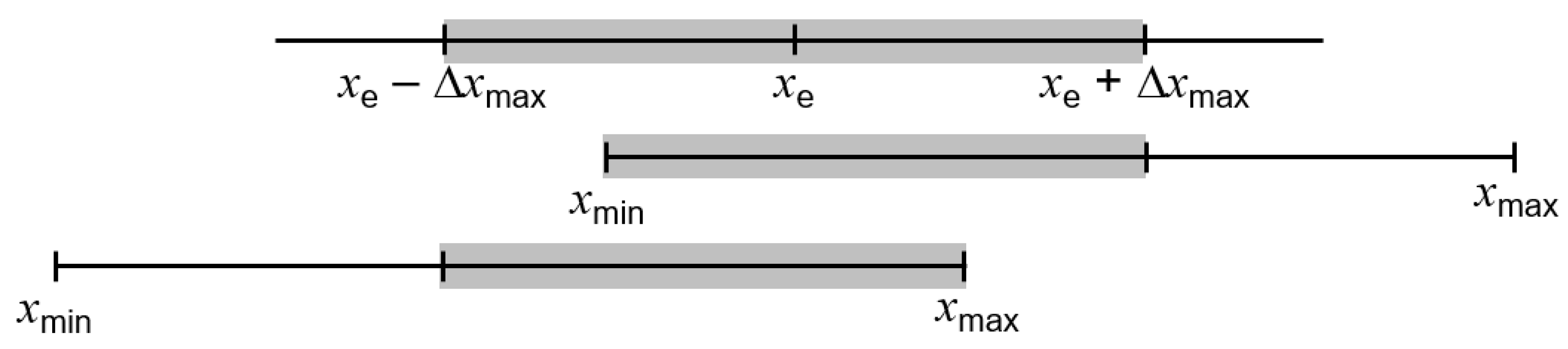
The design would not be changed when $D_e=1$ because the optimality condition is already satisfied. When $D_e<1$, it means that increasing design $x_e$ is less efficient in decreasing the compliance than increasing the volume. In this case, therefore, it is better to reduce $x_e$. When $D_e>1$, the opposite is true, and the design variable should increase. In addition, since it is not preferred to change a design significantly in one iteration, the maximum change in design $\Delta x_{\max }$ is also imposed. Figure 1 illustrates the possible ranges of design change. Starting from the current design $x_e$, the first case is when $[x_e-\Delta x_{\max },x_e+\Delta x_{\max }]\subset [x_{\min },x_{\max }]$. In this case, the design can be changed within the maximum change. The second case is when $x_e-\Delta x_{\max }<x_{\min }$. In this case, the design can be changed in $[x_{\min },x_e+\Delta x_{\max }]$. When $x_e+\Delta x_{\max }>x_{\max }$, the design can be changed in $[x_e-\Delta x_{\max },x_{\max }]$.

In the outer loop, the Lagrange multiplier is determined to satisfy the volume fraction constraint. The Matlab implementation of the 99-line topology optimization code [13] used a bisection method to find the Lagrange multiplier. Starting from the lower and upper bounds [0, 100,000] of the Lagrange multiplier, the range is halved every iteration of the outer loop, and the Lagrange multiplier takes the value in the middle of the range. With the current Lagrange multiplier, if the constraint is positive, $V(x)-f{V}_0>0$, then the upper half of the range is used in the next iteration; otherwise, the lower half is used. This bisection process is repeated until the range becomes less than a convergence tolerance.

For the purpose of generalizing the OCM, three obstacles must be overcome. The first obstacle is the compliance objective and the volume fraction constraint. First, the sensitivity of volume in Equation (3) is constant and independent of design. In addition, the sensitivity of compliance in Equation (2) can be calculated once the structural equilibrium is solved for $\left\{D\right\}$. Therefore, this particular combination of the objective and constraint has the almost free computation of sensitivities. However, the procedure cannot be generalized when there is more than one constraint.

The second obstacle is the assumption of sensitivities. In Equation (6), the OCM algorithm assumes that the objective derivative is negative and the constraint derivative is positive. This is true with the compliance objective and the volume fraction constraint. From Equation (2), the quadratic form ${\left\{d_e\right\}}^{\mathrm{T}}[k_e]\left\{d_e\right\}$ of a positive semi-definite stiffness matrix is always non-negative. Therefore, the compliance sensitivity in Equation (2) is always negative or zero. On the other hand, the volume fraction sensitivity in Equation (3) is constant and positive. In general optimization problems, it is possible that the objective may have a positive sensitivity for some designs, while a negative sensitivity for others. In particular, when there exists a design-dependent load, such as gravity, the sensitivity of compliance can be negative for some elements. Therefore, the design update formula in Equation (7) cannot be used as it is.

The third obstacle is the computational cost related to finding the Lagrange multiplier. As mentioned before, the Lagrange multiplier is determined through the bisection method, which requires hundreds of outer-loop iterations. When the number of design variables is large, this process can take a lot of computational time. The same is true for the method of moving asymptotes (MMA), where solving the MMA subproblem can be expensive especially when multiple constraints are active.

2.2. Generalized Optimality Criteria Method

The generalized optimality criteria (GOCM) method for topology optimization extends the capability of the OCM to multiple inequality constraints, possibly with improved computational efficiency. The general idea of OCM has been available for a long time in parameter optimization, albeit it was limited to minimizing weight with displacements, stresses, and natural frequencies [16,17]. The basic idea is to solve the Karush–Kuhn–Tucker condition, which is the necessary condition for optimization. The general optimization problem can be defined as

$$\begin{array}{ll}\mathrm{Minimize}\hfill & f(x)\hfill \\ \mathrm{subject}\hspace{0.17em}\hspace{0.17em}\mathrm{to}\hfill & g_i(x)\le 0,\hspace{1em}i=1,\dots ,NC\hfill \\ \hfill & [K]\left\{D\right\}=\left\{F\right\}\hfill \\ \hfill & x_{\min }\le x\le x_{\max }\hfill \end{array}$$

(8)

Even if a single objective function and only less-than-or-equal-to-type inequality constraints are used, it can easily be generalized to multiple objective functions with weighted sum and other types of constraints. In the following derivations, it is assumed that both the objective and constraints are normalized using the initial value and constraint bounds. For example, in the case of stress constraint given as $\sigma (x)\le {\sigma }_{\max }$ can be normalized as $g(x)=\sigma (x)/{\sigma }_{\max }-1\le 0$. In the case of the objective function, it can be normalized using the initial value.

In general, the constrained optimization problem can be converted into an unconstrained optimization problem using either the Lagrange multiplier method or penalty method. In the Lagrange multiplier method, the Lagrange function is defined by combining the objective function and constraints using Lagrange multipliers as

$$\mathrm{minimize}\hspace{0.17em}L(x,\lambda ,s)=f(x)+{\displaystyle \sum _{i=1}^{NC}{\lambda }_i(g_i(x)+s_i^2)}$$

(9)

where ${\lambda }_i$ is the Lagrange multiplier corresponding to constraint $g_i$. $s_i$ is called a slack variable, which is not zero when the constraint is inactive (i.e., less than zero).

The necessary condition for optimum is when the Lagrange function is stationary, i.e., its derivatives are zero. Since the Lagrange function has three variables, it is differentiated by all three variables as

$$\begin{array}{l}{\nabla }_{x}f(x)+{\displaystyle \sum _{i=1}^{NC}{\lambda }_i{\nabla }_x{g}_i}=0\\ g_i(x)+s_i^2=0,\hspace{1em}i=1,\dots ,NC\\ {\lambda }_i{s}_i=0\end{array}$$

(10)

where ${\nabla }_x=\partial /\partial x$ is the column vector of gradients. Due to the complementary slackness (i.e., switching condition), ${\lambda }_i{s}_i=0$, only the active constraints need to be considered in the necessary condition.

Since the second and third equations in Equation (10) are satisfied by identifying active constraints, the process of GOCM is to solve the first part of Equation (10). At an optimum design, the objective sensitivity can be represented by a linear combination of active constraint gradients. The coefficients in the linear combination are indeed the Lagrange multipliers. Since the Lagrange multipliers, ${\lambda }_i$, and design variables, $x$, are coupled, they have to be solved simultaneously. The challenge is that solving the nonlinear equation is computationally intensive and difficult due to numerical instability. The initial implementation of OCM by Sigmund [13] has a double-loop method, where the inner loop calculates the design variable, while the outer loop calculates the Lagrange multiplier. When multiple constraints are active, however, it would require multiple levels of loops to calculate the coupled equations.

The novel idea of the proposed GOCM is that the Lagrange multipliers do not have to satisfy Equation (10) at every iteration. Therefore, no iterative bisection is required to find the Lagrange multipliers. Instead, the Lagrange multipliers are updated at every optimization step so that when the optimization is converged, the necessary condition in Equation (10) is satisfied. Patnaik et al. [16] proposed several methods of updating the Lagrange multiplier.

Table 1. Lagrange multiplier update formulas.

Updating Methods	Updating Formulas
Linear form	${\lambda }_i^{k+1}={\lambda }_i^k(1+{\alpha }^k{p}_0{g}_i)$
Exponential form	${\lambda }_i^{k+1}={\lambda }_i^k{(g_i)}^{{\alpha }^k{p}_0}$
Inverse form	$\mathsf{\lambda }={[{\nabla }_x{g}^{\mathrm{T}}{\nabla }_{x}g]}^{-1}\left\{{\nabla }_x{g}^{\mathrm{T}}{\nabla }_{x}f\right\}$

summarizes the three updating schemes. In the table, $p_0$ is the initial value of an update parameter, and $\alpha$ is an acceleration parameter used to modify the update parameter. Patnaik et al. [16] suggested $p_0=0.5$ and $\alpha =1.0$.

In this article, the updating algorithm of the Lagrange multiplier is composed of two steps: (a) initial estimate and (b) update during iteration. First, the initial values of Lagrange multipliers are estimated using the inverse form in Table 1. However, it would be computationally complicated to calculate the inverse of the constraint gradient matrix, and it would be unnecessary as it provides the initial estimate. Instead, the uncoupled version of the inverse form is used for the initial estimate as

$${\lambda }_i=-\frac{{\nabla }_x{f}^{\mathrm{T}}{\nabla }_x{g}_i}{{\nabla }_x{g_i}^{\mathrm{T}}{\nabla }_x{g}_i}$$

(11)

The above estimate works well in most cases except when either the objective gradient or constraint gradients are zero or too small. In the optimization problem formulation, the objective function and constraints are normalized to the initial value and/or constraint limit. Therefore, the initial value of ${\lambda }_i=1$ is a good starting point when ${\nabla }_{x}f+\lambda {\nabla }_{x}g\approx 0$.

The basic concept of GOCM is when the constraint is violated, the Lagrange multiplier needs to increase, while it is decreased when the constraint is inactive. Therefore, a simple updating formula would be ${\lambda }_i^{k+1}={\lambda }_i^k(1+g_i^k)$. In this simple formula, the Lagrange multiplier increases when the constraint is positive (i.e., the constraint is violated) or it decreases when the constraint is negative (i.e., the constraint is inactive). This simple algorithm can cause some problems when the constraint violation is not recovered quickly, or the constraint is inactive for many steps. For example, if the constraint is violated a lot and stays violated for many steps, then the Lagrange multipliers can increase too fast. Therefore, it would be necessary to include the effect of change in constraint. In the article, the following updating rule is proposed for the Lagrange multiplier:

$${\lambda }_i^{k+1}={\lambda }_i^k[1+p_0(g_i^k+\Delta g_i^k)]$$

(12)

where $p_0$ is the update parameter similar to those used in Table 1. The update parameter can have a positive value when both the sign of $g_i^k$ and $\Delta g_i^k$ are the same. A more complex scheme can also be used, as shown in the Matlab code in Section 3.

The updating algorithm in Equation (12) is applied (a) when the current constraint is violated and the constraint increases from the previous step or (b) when the current constraint is inactive and the constraint continues to decrease. In order to make the updating process stable, the maximum change of the Lagrange multipliers is used. Moreover, the Lagrange multipliers are limited to change within the lower- and upper-bounds. Since all constraints are normalized by their bounds, the magnitudes of the Lagrange multipliers are in a similar order of magnitude.

In the theory of Lagrange multiplier, it is well known that it is zero when the constraint is not active, while it is positive when the constraint is active. That means, it is unnecessary to consider the Lagrange multiplier for inactive constraints and only active constraints are considered in the optimization. However, from a practical point of view, it is difficult to turn on and turn off constraints during optimization. Therefore, in the implementation, all constraints and Lagrange multipliers are retained. Then a constraint is inactive, the corresponding Lagrange multiplier will converge to its lower bound, which reduces its effect on the optimality criteria.

Once the Lagrange multipliers are updated, the next step of GOCM is to update design variables. When the optimization problem is composed of the compliance objective and volume fraction constraint, the scale factor $D_e$ in Equation (6) is used to update design variables. This updating algorithm is based on the assumption that that the objective sensitivity is negative, while the constraint sensitivity is positive. Similar algorithms for design variable update were available in Patnaik et al. [16], which are summarized in

Table 2. Design variable update formulas.

Methods	Formulas
Linear form	$x_e^{k+1}=x_e^k[1+(D_e-1)/({\beta }^k{q}_0)]$
Exponential form	$x_e^{k+1}=x_e^k{D}_e^{1/({\beta }^k{q}_0)}$
Reciprocal form	$x_e^{k+1}=x_e^k/[1-(D_e-1)/({\beta }^k{q}_0)]$

. All the formulas are based on the scale factor defined as

$$D_e=-\frac{{\displaystyle \sum _{i=0}^{NC}{\lambda }_i\frac{\partial g_i}{\partial x_e}}}{\frac{\partial f}{\partial x_e}}$$

(13)

Making $D_e=1$ is equivalent to the stationary condition of Karush–Kuhn–Tucker condition in Equation (10). The two acceleration parameters in Table 2 are suggested to be $q_0=2.0$ and $\beta =1.0$.

In order to consider the general objective and constraints, we need to modify the scale factor in Equation (13). For a given design variable (i.e., element), the scale factor is calculated on the basis of the sign of sensitivities. The numerator has all terms with negative sensitivities, while the denominator has all terms with positive sensitivities. Accordingly, the scale factor is calculated as

$$D_e=-\frac{{\langle \frac{\partial f}{\partial x_e}\rangle }_{-}+{\displaystyle \sum _{i=1}^{NC}{\lambda }_i{\langle \frac{\partial g_i}{\partial x_e}\rangle }_{-}}}{{\langle \frac{\partial f}{\partial x_e}\rangle }_{+}+{\displaystyle \sum _{i=1}^{NC}{\lambda }_i{\langle \frac{\partial g_i}{\partial x_e}\rangle }_{+}}}$$

(14)

where ${\langle a\rangle }_{-}=\min (0,a)$ and ${\langle a\rangle }_{+}=\max (0,a)$. When $D_e=1$, this formula will also satisfy the stationary condition of the Lagrange function. The only difference is that the original formulation calculates the scale factor on the basis of the ratio between objective sensitivity and the weighted sum of constraint sensitivities, while the proposed method uses the ratio between the positive and negative sensitivities. In the case of compliance objective and volume fraction constraint, Equations (6), (13), and (14) yield the identical scale factor.

In some special situations, the scale factor needs to be modified. If the numerator and/or the denominator are zero, the scale factor needs to be limited so that it stays close to one. Moreover, $D_e$ is scaled such that the design change in each iteration is less than $\Delta x_{\max }$. Once the scale factor is determined, Equation (7) is used to update the design variable.

3. Numerical Comparisons

In this section, the performance of the proposed GOCM algorithm is compared with the conventional algorithms, OCM and MMA. The first example is a direct comparison with the OCM using Sigmund’s 99-line Matlab code. The other examples are numerical comparisons with OCM and MMA using Autodesk Nastran.

3.1. Comparison with OCM

Since GOCM is directly related to OCM, it would make sense to compare the performance between the two. In this section, GOCM is implemented in the 99-line Matlab code. Although GOCM can handle different objectives and multiple constraints, this comparison is purely based on the compliance objective with volume fraction constraint.

In order to have an objective comparison, we modified the function OC (optimality criteria) to GOC for the purpose of GOCM.

• %%%%%%%%%% OPTIMALITY CRITERIA UPDATE %%%%%%%%%%%%%%%%%
• function [lmid,gl,xnew] = GOC(nelm,volfrac,lmid,gl,x,dc)
• eps = 0.05; move = 0.2;
• g = sum(sum(x))/(nelm*volfrac) − 1;
• dg = g − gl; gl = g;
• if (g > 0 && dg > 0) || (g < 0 && dg < 0), p0 = 1.0;
• elseif (g > 0 && dg > −eps) || (g < 0 && dg < eps), p0 = 0.5;
• else, p0 = 0;
• end
• lmid = lmid*(1 + p0*(g + dg));
• xnew = max(0.001,max(x − move,min(1.,min(x + move,x.*sqrt( − dc./(lmid/nelm))))));

In the code, lmid is the Lagrange multiplier with an initial value of 1.0, and gl is the normalized volume fraction constraint at the previous iteration, with an initial value of 0.0. These values are calculated in the GOC function and returned to the main program. The algorithm calculates the scale factor p0 using the normalized constraint, g, and its change, dg. In the main code, the sensitivity is scaled by the initial value of the compliance as dc = dc/f0, where f0 in the initial value of the compliance. In the same way, the sensitivity of the normalized volume fraction constraint becomes 1/nelm, where nelm is the number of design variables or the number of elements.

Figure 2a shows half of the MBB-beam that was used in Sigmund [13]. The design domain size is $100\times 50$, with the volume fraction constraint of 0.5. Accordingly, the following Matlab command-line is used to launch the topology optimization solver:

• top(100,50,0.5,3.0,1.5)

Figure 2b,c show the optimum designs from the OCM and GOCM algorithms, respectively, starting from the design domain and boundary conditions given in Figure 2a. Even if the two optimum designs are slightly different, they are very similar. The optimum objective functions (compliances) were found to be 79.18 (OCM) and 79.05 (GOCM). Therefore, GOCM found slightly smaller compliance than OCM. The number of optimization iterations is significantly different in that the OCM converged in 375 iterations, while GOCM in 166 iterations. However, this was the case in the specific example; other examples may have a different outcome. The major difference comes from the computational time for solving the optimality criteria. In order to have a fair comparison, we used Matlab tic and toc commands before and after calling the OC function. Since OCM takes more iterations, only the time up to 166 iterations were calculated. It turned out that the computational time of OCM took 10 times longer than that of GOCM. This is expected because OCM needs the bisection method to find the Lagrange multiplier, which normally requires hundreds of iterations, while the GOCM does not have any iteration.

Figure 3 shows the optimization histories for OCM and GOCM for the first 80 iterations. Both methods showed a similar convergence trend, but the OCM showed smooth variation because it enforced the equality constraint at every iteration. The OCM maintained $g(x)=0$ throughout all iterations, while the GOCM oscillated the positive and negative values until it was stabilized after the 50th iteration. The Lagrange multiplier was converged to 0.6166 (OCM) and 0.6126 (GOCM). This example shows that GOCM and OCM showed a similar optimization trend. However, the GOCM showed oscillation in early design but converged much faster. In addition, the design updating process of GOCM was 10 times faster than that of OCM.

3.2. Performance Comparison with OCM and MMA

The next example is the gripper-arm model, as shown in Figure 4a. The design domain of 127.6 × 43.1 × 10.3 mm³ was modeled by $135\times 46\times 11\approx 68,000$ elements. All nodes on the two holes were fixed, and a total of 222.41 N force was uniformly distributed on the upper-right edge as shown in the figure. For material, stainless steel 426 L was used with Young’s modulus of 193 GPa and Poisson’s ratio of 0.25.

In order to have a comparison using all three optimization algorithms, the optimization problem still uses the minimization of the compliance with volume fraction constraint, i.e., single objective and single constraint. Therefore, the optimization problem is defined as

$$\begin{array}{ll}\mathrm{Minimize}\hfill & c(x)={\displaystyle \sum _{e=1}^{N_e}{(x_e)}^p{\left\{d_e\right\}}^{\mathrm{T}}[k_e]\left\{d_e\right\}}\hfill \\ \mathrm{subject}\hspace{0.17em}\hspace{0.17em}\mathrm{to}\hfill & \frac{V(x)}{V_0}\le 0.09\hfill \\ \hfill & [K]\left\{D\right\}=\left\{F\right\}\hfill \\ \hfill & x_{\min }\le x\le x_{\max }\hfill \end{array}$$

(15)

It is noted that the volume fraction constraint allows only 9% of the material; therefore, most materials will be removed. The OCM uses the equality constraint, but both MMA and GOCM use the less-than-or-equal-to type constraint. Since the volume fraction constraint is active at the optimum design, both formulations would be identical.

The optimization problem was solved using Autodesk Nastran 2020 (Autodesk Inc., San Rafael, CA, USA) [19]. At each optimization iteration, using the current design variables, Autodesk Nastran calculated the structural responses, adjoint loads, adjoint responses, and sensitivity of objective and constraints. Then, using this information, the optimization algorithm calculated new design variables. This iteration was repeated until the convergence criteria were satisfied.

Figure 4b–d shows the optimum designs using three algorithms. Even if the optimum designs were slightly different, the objective and constraint were close to each other, as shown in

Table 3. Comparison of optimum designs using different optimization algorithms.

Algorithm	Iteration	Compliance	Volume Fraction	Total Time (s)	Algorithm Time (s)	Algorithm/Total Time (%)
OCM	102	1.728 × 10−2	0.09	554	33.16	6.0
MMA	102	1.710 × 10−2	0.09	788	166	21.0
GOCM	102	1.741 × 10−2	0.09	566	0.10	0.02

. The MMA algorithm tended to make smaller features than other algorithms, but this could be different if the optimization problem started from different initial densities. This was the fundamental limitation of gradient-based optimization, wherein only local optima could be found. An important distinction could be observed in computational times in the last two columns of Table 3. The total time is the time in seconds to solve the optimization problem, while the algorithm time is the time that is used in the optimization algorithm. While the MMA took 21% of computational time, the OCM and GOCM took 6% and 0.02%, respectively. The history of the compliance objective displayed in Figure 5 shows that the OCM showed a smooth variation of the objective, but none of the methods provided a monotonic change of the objective. In this particular example, both OCM and MMA converged to the optimum design from the feasible domain, while GOCM converged from the infeasible domain. It is also noted that the optimization history of MMA and GOCM showed a saw-tooth type pattern, which was not related to the optimization algorithm. Rather, it was related to the progressive increase of the penalty parameter in the SIMP algorithm.

3.3. Performance Comparison for Multiple Constraints

In this section, an optimization problem with multiple constraints is used to compare the performance of different algorithms. As mentioned before, when multiple constraints are present, the OCM cannot be used. Therefore, only MMA and GOCM algorithms can be used. The same gripper-arm model in the previous section was used for the comparison of MMA and GOCM when there were multiple constraints. The design optimization problem is defined as

$$\begin{array}{ll}\mathrm{Minimize}\hfill & c(x)={\displaystyle \sum _{e=1}^{N_e}{(x_e)}^p{\left\{d_e\right\}}^{\mathrm{T}}[k_e]\left\{d_e\right\}}\hfill \\ \begin{array}{l}\mathrm{subject}\hspace{0.17em}\hspace{0.17em}\mathrm{to}\\ \\ \\ \\ \\ \end{array}\hfill & \begin{array}{l}\frac{V(x)}{V_0}\le 0.09\\ {({\sigma }_{vM})}_{\max }\le 4.5\times {10}^7\\ u_{\max }\le 0.0001\\ v_{\max }\le 0.0001\\ w_{\max }\le 0.0001\end{array}\hfill \\ \hfill & [K]\left\{D\right\}=\left\{F\right\}\hfill \\ \hfill & x_{\min }\le x\le x_{\max }\hfill \end{array}$$

(16)

The compliance objective and volume fraction constraint are identical to the previous example. In addition, the maximum von Mises stress and the maximum displacement constraints were added. For the maximum von Mises stress, the aggregated P-norm stress was used [20]. For the displacement constraints, a similar P-norm was used to calculate the maximum displacement in each coordinate direction.

Figure 6a,b shows the optimum geometry using GOCM and MMA algorithms, respectively. Both methods took 102 iterations to converge, as shown in

Table 4. Comparison of optimum designs with multiple constraints.

Algorithm	MMA	GOCM
Iteration	102	102
Compliance	1.855 × 10−2	1.709 × 10−2
Volume fraction	0.09	0.09
Displacement (y)	1.0 × 10−4	0.96 × 10−4
Stress	4.5 × 107	4.3 × 107
Total time (s)	2541	1580
Algorithm time (s)	820	0.15
Algorithm/total time (%)	32.3	0.01

. In this optimization problem, GOCM found an optimum design whose compliance was about 8% less than that of MMA. Among five inequality constraints, the volume fraction, maximum y-displacement, and maximum von Mises stress were active at the optimum design. The MMA algorithm took 32% of the total time. Considering that the remaining 68% of the time was used for calculating structural response, adjoint load, adjoint response, and adjoint sensitivity, the optimization algorithm took a significant portion of the time. Compared to the MMA, the GOCM algorithm took a fraction of a second, which provides a significant advantage over MMA. It is interesting to note that the MMA algorithm became computationally expensive when constraints became active. As shown in Figure 7, initially the MMA algorithm took about 1.5 s for each iteration, but after the 40th iteration, it took about 15 s for each iteration, where constraints became active. This is because the MMA subproblem can be expensive when multiple constraints are active.

4. Conclusions

In this article, a new topology optimization algorithm, the generalized optimality criteria method (GOCM), was proposed. It is based on the conventional optimality criteria method (OCM), wherein both Lagrange multiplier and design variables are updated. The main difference is that the proposed method can have multiple inequality constraints, while the OCM can only support a single constraint (e.g., volume fraction). The Lagrange multipliers were updated on the basis of the constraint violation and constraint change. Then, the design variables were updated toward the direction to satisfy the optimality criteria. Therefore, constraints may not have been satisfied during the optimization iteration, but they were satisfied upon convergence. Numerical examples showed that the proposed method was faster than the OCM and the method of moving asymptotes (MMA). In the case of a MATLAB-based 2D model with 5000 design variables, GOCM was 10 times faster than OCM. In the case of the gripper-arm model (68,000 elements), GOCM was more than 1000 times faster than MMA and 330 times faster than OCM. When there were multiple constraints, the optimization time became comparable with that of finite element simulation times. In the case of MMA, the optimization algorithm time was about 35% of the total time, while the optimization time of GOCM was negligible. Therefore, the proposed method was versatile to handle multiple constraints, while computationally efficient.

For future research, it would be beneficial to handle active and inactive constraints separately. The current implementation updated the Lagrange multipliers for both active and inactive constraints, but it would be necessary to remove the effect of inactive constraints completely from optimality criteria. In GOCM, it is possible that constraints are consistently violated during iterations and only the final converged design satisfies the constraints. In order to make un-converged designs useful, it would be beneficial that designs are updated in the feasible region.

References

1. Bendsøe, M.P. Optimization of Structural Topology, Shape and Material; Springer: Berlin/Heidelberg, Germany, 1995. [Google Scholar]
2. Svanberg, K. The method of moving asymptotes—A new method for structural optimization. Int. J. Numer. Methods Eng. 1987, 24, 359–373. [Google Scholar] [CrossRef]
3. Dunning, P.D.; Kim, H.A. Introducing the sequential linear programming level-set method for topology optimization. Struct. Multidiscip. Optim. 2015, 51, 631–643. [Google Scholar] [CrossRef] [Green Version]
4. Siva, L.; Mahesh, N.; Sateesh, N. Topology optimization using solid isotropic material with penalization technique for additive manufacturing. Mater. Today Proc. 2017, 4, 1414–1422. [Google Scholar] [CrossRef]
5. Wang, S.; Tai, K. Structural topology design optimization using Genetic Algorithms with a bit-array representation. Comput. Methods Appl. Mech. Eng. 2005, 194, 3749–3770. [Google Scholar] [CrossRef]
6. Lynn, N.; Ali, M.; Suganthan, P. Population topologies for particle swarm optimization and differential evolution. Swarm Evol. Comput. 2018, 39, 24–35. [Google Scholar] [CrossRef]
7. Bureerat, S.; Limtragool, J. Structural topology optimisation using simulated annealing with multiresolution design variables. Finite Elements Anal. Des. 2008, 44, 738–747. [Google Scholar] [CrossRef]
8. Gao, F.; Han, L. Implementing the Nelder-Mead simplex algorithm with adaptive parameters. Comput. Optim. Appl. 2010, 51, 259–277. [Google Scholar] [CrossRef]
9. Haftka, R.T. Requirements for papers focusing on new or improved global optimization algorithms (Editorial). Struct. Multidiscip. Optim. 2016, 54, 1. [Google Scholar] [CrossRef] [Green Version]
10. Zhou, Y.; Saitou, K. Gradient-based multi-component topology optimization for stamped sheet metal assemblies (MTO-S). Struct. Multidiscip. Optim. 2018, 58, 83–94. [Google Scholar] [CrossRef]
11. Allaire, G. A review of adjoint methods for sensitivity analysis, uncertainty quantification and optimization in numerical codes. Ingénieurs l’Automobile SIA 2015, 836, 33–36. [Google Scholar]
12. Roosta, F.; Liu, Y.; Xu, P.; Mahoney, M. Newton-MR: Newton’s Method Without Smoothness or Convexity. arXiv 2018, arXiv:1810.00303. [Google Scholar]
13. Sigmund, O. A 99 line topology optimization code written Matlab. Struct. Multidiscip. Optim. 2016, 21, 120–127. [Google Scholar] [CrossRef]
14. Jiang, T.; Papalambros, P.Y. A first order method of moving asymptotes for structural optimization. Trans. Build Environ. 1995, 13, 75–83. [Google Scholar]
15. Arora, J.S. Introduction to Optimal Design; McGraw-Hill: New York, NY, USA, 1988. [Google Scholar]
16. Patnaik, S.N.; Guptill, J.D.; Berke, L. Merits and Limitations of Optimality Criteria Method for Structural Optimization; NASA Technical Paper 3373; National Aeronautics and Space Administration: Cleveland, OH, USA, 1993. [Google Scholar]
17. Berke, L.; Khot, N.S. Structural optimization using optimality criteria. Comput. Aided Optim. Des. Struct. Mech. Syst. 1987, 27, 271–311. [Google Scholar]
18. Sands, T. Optimization Provenance of Whiplash Compensation for Flexible Space Robotics. Aerospace 2019, 6, 93. [Google Scholar] [CrossRef] [Green Version]
19. Weinberg, D.J. Autodesk Inventor Nastran 2020 User’s Manual; Autodesk Inc.: San Rafael, CA, USA, 2019. [Google Scholar]
20. Park, Y.K. Extensions of Optimal Layout Design Using the Homogenization Method. Ph.D. Thesis, University of Michigan, Ann Arbor, MI, USA, 1995. [Google Scholar]
Figure 1. Possible ranges of design change in the optimality criteria method.
Applsci 11 03175 g001
Figure 2. Design domain and optimum designs of a cantilevered beam.
Applsci 11 03175 g002
Figure 3. Design optimization histories for optimality criteria method (OCM) and generalized optimality criteria method (GOCM).
Applsci 11 03175 g003
Figure 4. The initial design domain and optimum designs using different methods for the gripper-arm model.
Applsci 11 03175 g004
Figure 5. Optimization history of compliance using three optimization algorithms.
Applsci 11 03175 g005
Figure 6. Optimum design of the gripper-arm model with multiple constraints.
Applsci 11 03175 g006
Figure 7. Accumulated optimization algorithm time for the method of moving asymptotes (MMA).
Applsci 11 03175 g007