High-Fidelity Fin–Actuator System Modeling and Aeroelastic Analysis Considering Friction Effect

Featured Application

A high fidelity aeroelastic model of a typical fin–actuator system is established, in which the friction model is more accurate. The influence of freeplay and friction on the system stability is analyzed using the time-domain method and frequency-domain method, and some suggestions for flutter suppression design are put forward.

Abstract

Both the dynamic characteristics and structural nonlinearities of an actuator will affect the flutter boundary of a fin–actuator system. The actuator models used in past research are not universal, the accuracy is difficult to guarantee, and the consideration of nonlinearity is not adequate. Based on modularization, a high-fidelity modeling method for an actuator is proposed in this paper. This model considers both freeplay and friction, which is easy to expand. It can be directly used to analyze actuator characteristics and perform aeroelastic analysis of fin–actuator systems. Friction can improve the aeroelastic stability, but the mechanism of its influence on the aeroelastic characteristics of the system has not been reported. In this paper, the LuGre model, which can better reflect the friction characteristics, was integrated into the actuator. The influence of the initial condition, freeplay, and friction on the aeroelastic characteristics of the system was analyzed. The comparison of the results with the previous research shows that oversimplified friction models are not accurate enough to reflect the mechanism of friction’s influence. By changing the loads, material, and geometry of contact surfaces, flutter can be effectively suppressed, and the power loss caused by friction can be minimized.

1. Introduction

Flutter is a critical problem in modern flight vehicle design. To pursue lighter weight, wings and control surfaces tend to be more flexible, which may lead to flutter. Flutter instability will seriously affect aircraft performance and flight safety [1]. The conventional aeroelastic analysis of the control surface often focused only on the surface itself, and the actuator supporting the surface was regarded as a linear torsion spring with constant stiffness [2], as shown in Figure 1a. In fact, many experiments have proved that the actuator itself has dynamic characteristics, especially electromechanical servo actuators. Electromechanical servo actuators have good maintainability, low static power consumption, and storage convenience, so they have been widely used in missile control fin position servo systems [3]. Thus, they are the modeling objects of this paper. An electromechanical actuator consists of multiple components that can be classified as the moment of inertia (MOI), elastic spring, and damper, as shown in Figure 1b, which means that the actuator should not be over-simplified as a linear spring. Moreover, the stiffness of the actuator will change according to the change in the external load, which is called dynamic stiffness. In addition, the actuator has control algorithms and electrical and mechanical nonlinearities such as current/voltage saturation, freeplay, and friction [4]. The analysis of the fin–actuator system, considering the dynamic characteristics of the actuating system, makes the results different from those of wings only [5], which will affect the flutter boundary of the system.

Both the dynamics and structural nonlinearity of the actuator will greatly affect the aeroelastic characteristics of the system [6,7]. In the field of aeroelasticity, there are some studies that model the actuator and perform flutter analysis while considering the actuator dynamics and structural nonlinearities. Yehezkely et al. [5] performed an aeroelastic analysis of the missile fin with a nonlinear pneumatic actuator and proposed a flutter suppression method. Paek and the team [8] analyzed the flutter characteristics of the control fin of a rocket considering dynamic actuator characteristics. Shin et al. [6] established a basic framework for obtaining the aeroelastic stability results of a fin–actuator system considering the actuator’s dynamic characteristics. They found that the flutter boundary could be increased in this way. In the same year, Shin et al. [9] investigated the same system with the consideration of actuator nonlinearities, such as freeplay, backlash, and transmission error. The results show that both the freeplay and backlash may influence the actuator dynamic stiffness. They also found that the nonlinearity and gear reductions can greatly affect the limit cycle oscillation (LCO) characteristics. Yang et al. [7] obtained the aeroelastic characteristics of the fin–actuator system containing preload freeplay and found that an appropriate preload angle can suppress LCOs. Zhang and his team [10] analyzed the influence of actuator parameters on the dynamic stiffness. The results show that factors such as inertia of the motor rotor, connection stiffness between different levels of reducers, reduction ratio of each level of reducer, and the damping at the actuator fin shaft have significant effects. It can be seen that the studies above only considered freeplay or other nonlinearities in the actuator and rarely analyzed the friction. Friction actually has a great influence on aeroelastic properties, which exists widely and can be used to improve aeroelastic properties. Therefore, it was innovative and necessary to add a friction nonlinearity module to the model in this paper. Moreover, the previous work was only for a specific actuator, which is often too simplified, and the reliability of the model was not easy to guarantee. Furthermore, they often used the dynamic differential equations of the actuator to carry out modeling and analysis. The coupling between these equations often makes the modeling process cumbersome and the solving process complex. Therefore, a new actuator modeling method is needed. Based on modularization, a high-fidelity and systematic modeling method for an actuator is formed that can ensure accuracy, ease of use, and consider freeplay and friction at the same time. It can be easily extended to different configurations of actuators. Using this model, the characteristics of the actuator can be obtained directly for the analysis of aeroservoelasticity.

In addition to the natural friction at the joints of the system, engineers, based on experience, take measures to increase friction in order to suppress flutter. For example, friction sheets [11] or friction rings [12] were added to some actuators to increase friction. Friction plays a positive role in the aeroelastic system, but friction in servomechanism systems dissipates power [13] and may cause position signal steady-state errors or oscillations. The added friction sheet is often set empirically. So far, the mechanism of friction on the aeroelastic characteristics of the system is still unclear, and relevant research or analysis has not been reported. How can we reduce friction while ensuring the effect of friction on flutter stability? How can we achieve a balance between ensuring aeroelastic stability and reducing power loss? These are the issues that this article explores in the study of the friction influence mechanism.

Friction is a nonlinear and complex phenomenon that is determined by the relative motion between the two contact surfaces. Friction is related to interface material and operating conditions, such as loads acting on the contact [14]. Introducing nonlinearity significantly complicates all aspects of already complicated aeroelastic equations of motion, to the point that friction is typically omitted from a flutter-related analytical workflow or approximated by a constant value. Some researchers use simple friction models to analyze the influence of friction on aeroelastic characteristics. Khalak [15] researched stability criteria with consideration of mechanical damping, which was assumed constant. Griffin et al. [16] considered friction as a hysteretic spring with damping to study the blade response. The blade was simplified as a single degree of freedom system, and then the maximum response amplitude of it was analyzed using the Ritz method. Whiteman and the team [17] studied the possibility of dry friction for flutter suppression. The results showed that the aeroelastic stability boundary can be enhanced by changing the position of friction and the geometry of the interfaces. Mignolet et al. [18] validated for the first time that friction may play a stabilizing role in LCOs that occur after flutter. Tan et al. [19] studied the stability of an aeroelastic system with 1.5 degrees of freedom. The results showed that different friction stiffness has an influence on the critical aerodynamic damping ratio and the stability boundary of the system, but it has little influence on the stability boundary. Lu et al. [20] studied the effect of the Coulomb friction on airfoil aeroelastic stability by a numerical method and the harmonic balance method. The results showed that Coulomb friction can increase the flutter velocity, and it is affected by the initial condition. Wayhs-Lopes et al. [21] regarded Coulomb friction as a linear damping ratio and analyzed the influence of the Coulomb friction on LCOs caused by symmetric and asymmetric freeplay. The results show that friction is dissipative, but it is not enough to restrain LCOs. The friction model used in the above work is relatively simple and is a preliminary exploration of the friction effect mechanism and cannot fully reflect the friction characteristics. Therefore, the prediction of the stability boundary of a fin–actuator aeroelastic system is not enough. In fact, in engineering, the friction can be changed by adjusting the preload, the roughness of the friction surface, lubrication, material, temperature, and other factors that cannot be represented fully by simple models. Therefore, a model that can more accurately reflect the friction characteristics is introduced into the aeroelastic analysis model to improve the model’s accuracy, study further the influence mechanism of the above factors on the aeroelastic stability, and give some guidance suggestions.

The friction models that are currently used are mainly separated into two main types: the static model and the dynamic model [22]. The static model may include different components such as viscous friction, Coulomb friction, the Stribeck effect, and static friction. However, the static friction model cannot describe the influence of friction when the contact surfaces are relatively static. Some experiments show that some phenomena of friction can only be reproduced by dynamic models with memory, such as hysteresis, rate-dependence, and pre-displacement. The dynamic friction model can reflect the friction phenomenon more accurately, and therefore has more application value. Many researchers have developed a variety of dynamic models, mainly including the Dahl model [23], the LuGre model [24,25], the Leuven model [26,27], the Generalized Maxwell-Slip (GMS) model [28,29], and two-state friction model (2SEP) [30]. The Dahl model is not accurate enough when the velocity is low, and it cannot capture stick-slip motion. The LuGre friction model extends the Dahl model, which was proposed by Canudas de Wit and his companions [24,25,31,32,33,34]. It can reflect the complex processes of friction static and dynamic characteristics, including viscous friction, Stribeck effect, variable static friction, memorial friction, and pre-sliding displacement. The disadvantage of the LuGre model is that the hysteresis behavior does not have nonlocal memory characteristics in the pre-sliding regime, which has attracted some attention in the field of precise control. The Leuven model can reflect this characteristic, but it is difficult to implement. The same author also proposed the GMS model. Compared with the Leuven model, the GMS model can more accurately reflect the physical mechanism of friction, but the model is also more complex, which leads to difficulties in implementation or identification. The 2SEP model considers to a greater extent the micro-scale elastoplasticity, which is not the focus of this paper. A comparison of these models is shown in

Table 1. Friction characteristics reflected by different models. Generalized Maxwell-Slip, GMS; two-state friction model, 2SEP.

	Viscous	Stribeck Effect	Pre-Sliding	Hysteresis
Coulomb	No	No	No	No
Viscous	Yes	No	No	No
Stribeck	Yes	Yes	No	No
Dahl	No	No	Yes	Yes
LuGre	Yes	Yes	Yes	Yes
Leuven	Yes	Yes	Yes	Yes
GMS	Yes	Yes	Yes	Yes
2SEP	Yes	Yes	Yes	Yes

.

It is worth noting that when choosing a model, a proper trade-off must be made between model fidelity and implementation. The accuracy of the LuGre model is sufficient for the problem we want to study. The parameters’ physical meaning of the LuGre model is clear, and thus can easily match experimental data. It is a first-order model, which is more convenient to use and analyze than other second-order models [35]. Various benefits make this model widely used in control systems [36,37,38,39,40], which means it is easy to integrate into the actuator model based on SIMULINK, launched by MathWorks company, and it is also convenient for subsequent work with which to perform active flutter suppression. Using more complex models to consider the effect of friction in a more micro and accurate way can be an open question for future investigations.

The LuGre model contains only six parameters, which are ${\sigma }_0$, ${\sigma }_1$, ${\sigma }_2$, $F_{\mathrm{c}}$, $F_{\mathrm{s}}$, and $V_{\mathrm{s}}$. Many researchers have proposed effective LuGre parameters identification methods [31,41,42,43]. Based on interpreting the asperities contact, the LuGre model uses elastic spring-like bristles with damping to accurately represent the asperities between two contact surfaces. ${\sigma }_0$ is the stiffness of the assumed elastic spring, and ${\sigma }_1$ is the damping that is associated with micro-displacement. The bristles deform because of the action of external force, and the sum of the force generated by bristles’ deformation plus the viscous friction represents the friction force [44]. The average deformation of the bristles reflects the characteristics of dynamic friction. Once the bristles reach their maximum deformation, which also means friction force has been larger than the maximum static friction force $F_{\mathrm{s}}$, slip starts, as illustrated by the schematic representation in Figure 2.

In this article, a high-fidelity simulation model of a typical electromechanical actuator was established, considering its structural characteristics, details of servomechanism, freeplay, and friction. The actuator was divided into modules to solve the problem that the previous model was not universal and extensible. Then the fin–actuator system was established by connecting the actuator with the fin using the branch mode method. The unsteady aerodynamic force acted on the control fin. The influence on the system of freeplay and friction was studied using numerical simulation. Compared with previous literature, the friction model used in this paper could better reflect the real physical phenomenon, and the mechanism of friction effect on aeroelastic system was studied. Based on the results, some guidelines applicable to engineering projects are put forward.

This paper is organized as follows. Section 2 shows the study object of this article, which is a typical fin–actuator system with a friction sheet. Section 3 presents the high-fidelity modeling method of a fin–actuator system considering aerodynamics. The frequency domain and time domain flutter analysis methods are established in Section 4. Section 5 introduces the results and discussion of the stability analysis of the fin–actuator system, considering freeplay and friction nonlinearity of the actuator, and proposes some rules for the design reference of flutter suppression.

2. Study Object

The electromechanical actuator used in this paper was composed of a DC motor, a primary gear reducer, a lead screw–nut pair, a fork, a controller, and a sensor. Figure 3a shows the whole structure of the fin–actuator system. The fork between the screw and the fin shaft drove the fin. A friction sheet was installed under the fork as shown in Figure 3b. The mutual extrusion of the sheet and the fork produced the friction force, which caused the friction torque relative to the center of the fin shaft. One bolt fastened one section of the friction sheet, and the other bolt, which can provide a pressing force changed artificially, pressed the other section. Adjusting the pressure applied by the screw to the friction sheet, changing the materials in contact, or changing the roughness of the contact surface between the sheet and the fork could regulate friction.

The MOI of the fin was 0.0105 kg·m². A branch mode analysis of the fin was performed, which was adopted for aeroelastic analysis, and the first two elastic natural frequencies and the corresponding mode shapes of branch 1 are listed in

Table 2. Elastic modal frequencies and modal shapes of the fin.

Elastic Branch	Frequency	Modal Shape
1st mode	50.3 Hz
2nd mode	593.0 Hz

.

3. Modeling of the System

The electromechanical actuator installed on a missile provides sufficient torque to rotate the control fin against aerodynamic loads and allows the fin to follow guidance commands. The actuator must have appropriate stiffness to offset the disturbance to meet the stability and accuracy requirements. Different support stiffnesses will change the natural mode of the fin. Therefore, the normal mode cannot effectively represent the fin. To model the motion of the system, the substructure technique was introduced.

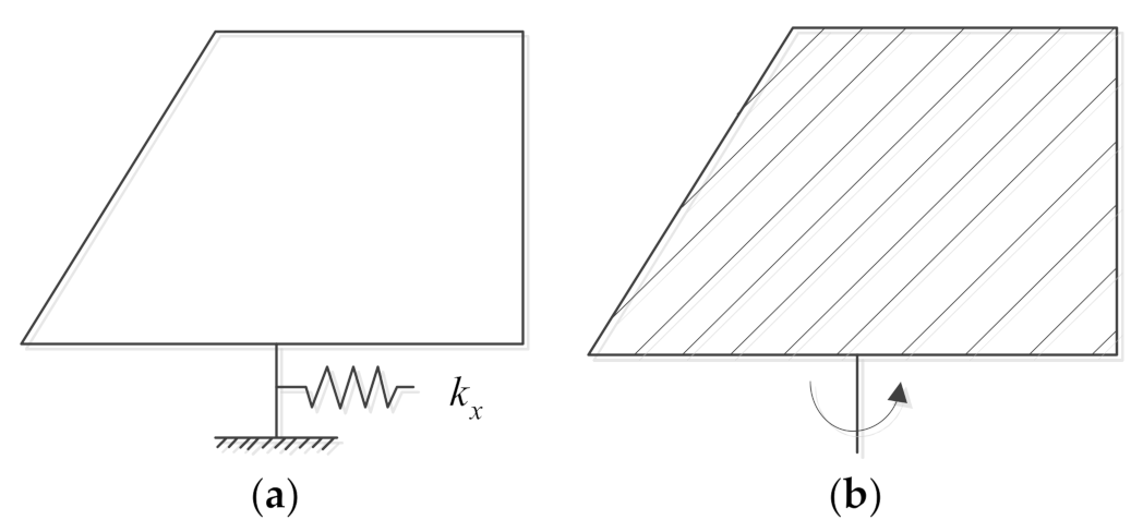
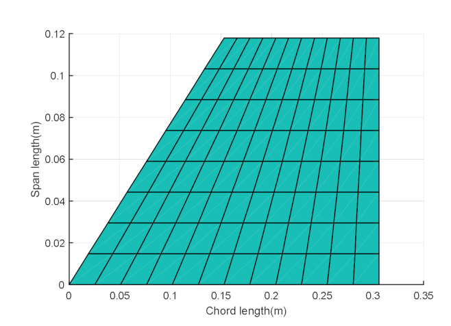
3.1. Modeling of the Fin Structure

Here, the Gladwell branch modal synthesis method was applied and used to model the fin structure. This method divides the modes into two branches—namely, the elastic branch and the rotational rigid branch [10,45,46], as illustrated by the schematic diagram in Figure 4. Note that the elastic modal branch, which is branch 1, was obtained by adding a spring to the root of the fin shaft in the direction of the x axis and the fin was clamped in the y and z directions.

The dynamic equation of the fin structure is [47]:

$$M\ddot{x}+C\dot{x}+Kx=F$$

(1)

for which the details of matrix $M$, $C$, $K$, and $F$ are shown in Appendix A. Moreover, the generalized coordinates vector is $x^{\mathrm{T}}=[q_{\mathrm{e}},\delta ]$, where $q_{\mathrm{e}}$ is the displacement vector in generalized coordinates of elastic modes, and $\delta$ is the rotation angle of the actuator output shaft.

3.2. Modeling of the Unsteady Aerodynamics

The aerodynamic forces were calculated by the panel method. The reference Mach number was 2.5, and the air density was 1.225 ${\mathrm{kg}/\mathrm{m}}^3$ The aerodynamic influence coefficient (AIC) matrix was generated using ZONA7 [48]. Figure 5 shows the aerodynamic model of the fin.

The generalized aerodynamic forces in frequency domain can be written as follows:

$$f_{\mathrm{aero}}=q_{\infty }Ax$$

(2)

The details of $q_{\infty }$, $A$, and $x$ are shown in Appendix A.

3.3. State-Space Form of the Fin Model

Combining Equations (1) and (2), yields:

$$M\ddot{x}+C\dot{x}+Kx=f_{\mathrm{aero}}+f$$

(3)

where $f^{\mathrm{T}}=[\mathbf{0},M_{\mathrm{t}}]=[\mathbf{0},1]M_{\mathrm{t}}$.

The fin model in state-space form is:

$$\begin{array}{l}{\dot{x}}_{\mathrm{s}}=A_{\mathrm{s}}{x}_{\mathrm{s}}+B_{\mathrm{s}}{u}_{\mathrm{s}}\\ y_{\mathrm{s}}=C_{\mathrm{s}}{x}_{\mathrm{s}}+D_{\mathrm{s}}{u}_{\mathrm{s}}\end{array}$$

(4)

where the state vector is $x_{\mathrm{s}}{}^{\mathrm{T}}=[x,\dot{x},x_{\mathrm{a}}]$, $x_{\mathrm{a}}$ is the vector of $m$ augmented states. Input vector is $u_{\mathrm{s}}=M_{\mathrm{t}}$, and output vector is $y_{\mathrm{s}}{}^{\mathrm{T}}=[\delta ,\dot{\delta }]$. The size of $x$ is $(r+1+m)\times 1$, where $r$ represents the number of elastic natural modes of branch 1. Other matrices can be found in Appendix A.

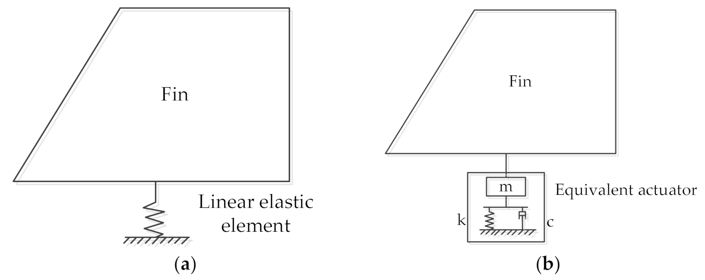
3.4. Modeling of the Electromechanical Actuator

To model the actuator, some generally accepted simplifications are used concerning power supplies, electromagnetic circuits, machine structures, and physical properties. The motor model directly relates the current and the output torque. The gearing mechanism and the lead screw–nut pair can be treated as mass-damping-spring systems to study their properties.

3.4.1. Model of DC Motor

Modeling of a DC motor ignores the details of the three-phase electromagnetic field and establishes the relationship between current and torque directly. The Lorentz force of the motor is given by:

$$T_{\mathrm{m}}=i{K}_{\mathrm{m}}$$

(5)

where $K_{\mathrm{m}}$ is the torque coefficient.

The motor winding voltage balance equation is given by:

$$iR+L\frac{di}{dt}=u_{\mathrm{m}}-C_{\mathrm{e}}{\dot{\theta }}_0-K_{\mathrm{i}}i$$

(6)

where $L$ is the inductance, $R$ is the resistance, $C_{\mathrm{e}}$ is the back electromotive force (EMF) coefficient, $u_{\mathrm{m}}$ is the driving voltage, $K_{\mathrm{i}}$ is the current feedback coefficient, ${\theta }_0$ is the angle of motor shaft.

The dynamic equation of motor rotor is given by

$$J_{\mathrm{m}}{\ddot{\theta }}_0=T_{\mathrm{m}}-b_{\mathrm{m}}{\dot{\theta }}_0+T_0$$

(7)

where $J_{\mathrm{m}}$ is the MOI of the rotor, $b_{\mathrm{m}}$ is the viscous damping coefficient of the rotor, $T_0$ is the load torque acting on the motor shaft, and its sign is defined as positive in the same direction as ${\theta }_0$.

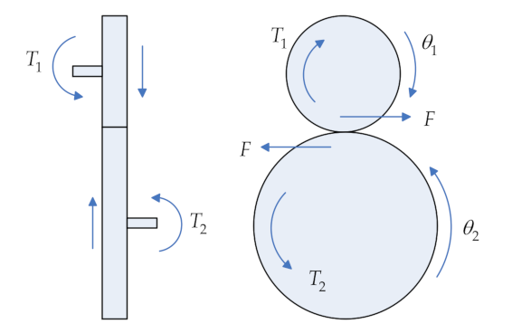
3.4.2. Model of the Gear Pair

What is connected to the DC motor is the gear pair. It should be noticed that the connection stiffness $k_{\mathrm{m}}$ exists between the motor and the gear pair.

The force diagram of gears is shown in Figure 6.

The dynamic equations of gears are given by:

$$J_1{\ddot{\theta }}_1+b_1{\dot{\theta }}_1=T_1-F{r}_1$$

(8)

$$J_2{\ddot{\theta }}_2+b_2{\dot{\theta }}_2=T_2+F{r}_2$$

(9)

where ${\theta }_1$ and ${\theta }_2$ are the rotation angles of the two gears, respectively; $J_1$ and $J_2$ are the MOIs of the two gears, respectively; $b_1$ and $b_2$ are the viscous damping coefficients of the two gears, respectively; $T_1$ and $T_2$ are the external moments acting on gears 1 and 2, respectively; $r_1$ and $r_2$ are the radii of the two gears, respectively; and $F$ is the force between gears 1 and 2. The meshing stiffness between gears is $k_{\mathrm{g}}$. The equation reflecting the relationship is given by:

$$F=k_{\mathrm{g}}\left({\theta }_1{r}_1-{\theta }_2{r}_2\right)$$

(10)

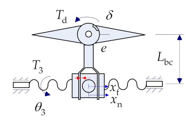
3.4.3. Model of the Screw–Nut Pair and Fork

The structure of the screw–nut pair which is connected to the gear pair is shown in Figure 7. The force of the screw–nut pair and fork model was complicated. Freeplay existed in the entire actuator. The screw–nut pair and fork model was the section closest to the actuator output shaft, with dynamic characteristics that will have a huge impact on the dynamic stiffness of the actuator. Therefore, in this paper freeplay was considered here as the comprehensive freeplay of the whole actuator. The friction produced by the friction sheet is described in this section, compared with the friction in other parts of the actuator, which was negligible.

The dynamic equations of the screw–nut pair and fork are given by:

$$\begin{array}{l}{J}_{\mathrm{sg}}{\ddot{\theta }}_3+b_3{\dot{\theta }}_3=T_3-F\tan \lambda r_{\mathrm{sg}}/\eta \\ F=k_{\mathrm{c}}\mathsf{\Delta }x\\ \mathsf{\Delta }x=x_{\mathrm{n}}-x_{\mathrm{f}}\\ x_{\mathrm{n}}={\theta }_3{r}_{\mathrm{sg}}\tan \lambda \\ x_{\mathrm{f}}=L_{\mathrm{bc}}\tan {\delta }_{\mathrm{e}}\\ {\delta }_{\mathrm{e}}=\left\{\begin{array}{c}\left(\left|\delta \right|-e\right)\mathrm{sgn}\left(\delta \right)\\ 0\end{array}\right.\begin{array}{c}\left|\delta \right|>e\\ \left|\delta \right|\le e\end{array}\\ T_{\mathrm{d}}=L_{\mathrm{bc}}F\end{array}$$

(11)

where ${\theta }_3$ is the screw rotation angular displacement, $b_3$ is the viscous damping coefficient of the screw, $\eta$ is the efficiency of the screw–nut pair, $\lambda$ is the helix angle of the lead screw, $r_{\mathrm{sg}}$ is the radius of the screw, $k_{\mathrm{c}}$ is the comprehensive stiffness between the screw–nut pair, $x_{\mathrm{n}}$ is the displacement of the nut, $x_{\mathrm{f}}$ is the displacement of the fork, $e$ is half the width of symmetrical freeplay at the fin shaft, $L_{\mathrm{bc}}$ is the length of the fork, ${\delta }_{\mathrm{e}}$ is the effective rotation angle of the actuator output shaft, and $T_{\mathrm{d}}$ is the output torque of the fork.

Notice that the connection stiffness between the gear pair and the screw–nut pair and fork is $k_{\mathrm{z}}$. Therefore $T_3$ is given by

$$T_3=-T_2=k_{\mathrm{z}}\left({\theta }_2-{\theta }_3\right)$$

(12)

As described in Section 1 (Introduction), a friction sheet is installed on the fork. Before the actuator starts to work, a certain pressure is applied to the friction sheet. The friction torque of the LuGre model is [49]:

$$\begin{array}{l}\dot{z}=\dot{\delta }-\frac{{\sigma }_0\left|\dot{\delta }\right|}{g(\dot{\delta })}z\\ g(\dot{\delta })=F_{\mathrm{c}}+\left(F_{\mathrm{s}}-F_{\mathrm{c}}\right)e^{-{(\frac{\dot{\delta }}{V_{\mathrm{s}}})}^2}\\ T_{\mathrm{f}}={\sigma }_{0}z+{\sigma }_1\dot{z}+{\sigma }_2\dot{\delta }\end{array}$$

(13)

where $T_{\mathrm{f}}$ is the friction torque; ${\sigma }_0$ and ${\sigma }_1$ have been explained in Section 1. ${\sigma }_2$ is the viscous damping coefficient, and z is an internal state variable that is introduced to represent the average deflection of all the bristles. The positive function $g(\dot{\delta })$ represents the Stribeck effect and Coulomb friction, which is related to several factors, such as temperature and material. $F_{\mathrm{c}}$ is Coulomb friction, and $F_{\mathrm{s}}$ corresponds to the maximum static friction. $V_{\mathrm{s}}$ is the Stribeck velocity, which reflects how fast friction approaches $F_{\mathrm{c}}$.

The torque of the actuator to the fin is given by

$$T_{\mathrm{fin}}=T_{\mathrm{d}}-T_{\mathrm{f}}$$

(14)

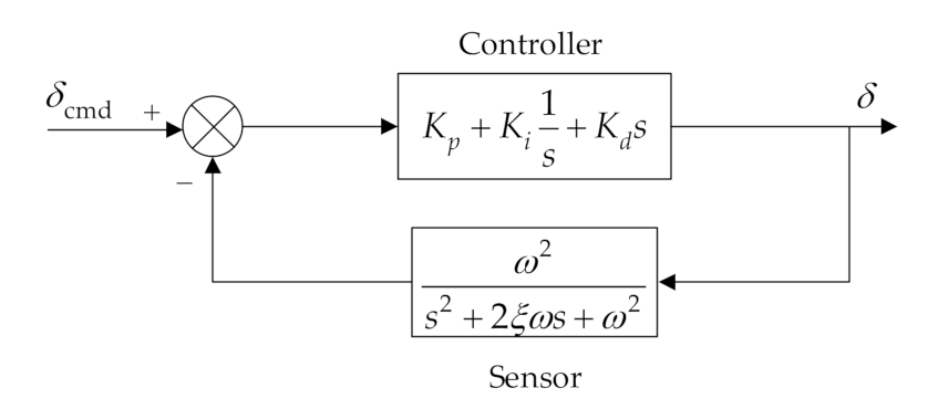
3.4.4. Model of the Controller and Sensor

The fin deflection angle is measured with an angular displacement sensor that gives position feedback to the controller. The transfer function of the sensor can be considered as a second-order element, which is given by:

$$G(s)=\frac{{\omega }^2}{s^2+2\xi \omega s+{\omega }^2}$$

(15)

The controller is used to adjust the input signal so that the output signal of the actuator can keep the track of the command signal. The most commonly used control law is to control the error between the command signal and the measured signal using proportional (P), integral (I), and derivative (D) terms [50]. The conventional actuator is a closed-loop system, and its controller usually includes amplification, filtering, and a PID control. The principle diagram of a PID control is shown in Figure 8, where ${\delta }_{\mathrm{cmd}}$ is the command signal.

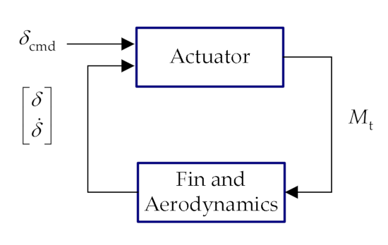
3.4.5. Model of the System

The actuator drives the fin to rotate and provides support stiffness for the fin in the meantime. The output of the actuator is the input of the fin and vice versa. Therefore, $M_{\mathrm{t}}=T_{\mathrm{fin}}$. A schematic diagram of the fin–actuator system is presented in Figure 9.

4. Flutter Analysis Method

4.1. Frequency Domain Method

4.1.1. Dynamic Stiffness

The describing function (DF) method is widely used in control engineering. Nikolay Mitrofanovich Krylov and Bogoliubov developed the DF method in the 1930s [51,52]. They used the average method and introduced the concept of equivalent linearization. Ralph Kochenburger extended the DF method [53]. When using the DF method, the Fourier coefficients of the nonlinear term need to be calculated and divided into two terms, which are respectively interpreted as the equivalent stiffness and damping terms related to the excitation signal. In order to ensure the quasi-linearity of the actuator, the excitation signal amplitude needs to be small enough. The actuator dynamic stiffness is essentially the transfer function of the quasi-linear actuator model obtained by the DF method when the input amplitude is small. Dynamic stiffness performance reflects the robustness of the actuator to disturbance. It refers to the dynamic torque required to be applied to produce a unit angle at the output shaft of the actuator. Dynamic stiffness reflects the characteristic that the support stiffness provided by the actuator to the fin will change with the frequency of the external load. As shown in Figure 10, the dynamic stiffness of the actuator is given by:

$$k_{\delta \delta }(\omega )=\frac{T_{\mathrm{load}}(\omega )}{{\theta }_{\mathrm{out}}(\omega )}=\overline{k_{\delta \delta }}{e}^{i\phi }$$

(16)

where $T_{\mathrm{load}}(\omega )=\overline{T_{\mathrm{load}}}{e}^{i\omega t}$ is the external load on the actuator output shaft, and ${\theta }_{\mathrm{out}}(\omega )=\overline{{\theta }_{\mathrm{out}}}{e}^{i(\omega t-\phi )}$ is the rotation angle of the actuator output shaft. The dynamic stiffness can be expressed by the amplitude phase curve varying with the input frequency $\omega$; $\overline{k_{\delta \delta }}$ is the amplitude and $\phi$ is the phase.

According to the relationship between the output and input power spectral densities (PSDs), the actuator dynamic stiffness can be calculated [6]. Taking the external load as the input signal $x(t)$ and the deflection angle as the output signal $y(t)$, the transfer function is:

$$k_{\delta \delta }(\omega )=\frac{P_{xy}(\omega )}{P_{xx}(\omega )}$$

(17)

where $P_{xy}(\omega )$ is cross PSD of $x(t)$ and $y(t)$, and $P_{xx}(\omega )$ is auto PSD of $x(t)$.

In numerical simulation, the excitation signal is a constant-amplitude sweep frequency signal, and the sweep frequency range should include the frequency range of interest. Another method to obtain dynamic stiffness is to combine a step sine sweep (SSS) signal with a least square (LS) frequency response function (FRF) estimation algorithm. The SSS signal contains considerable energy to excite out all the characteristics of the actuator, and the LS algorithm is an averaging process in a sense and essentially plays an effective filtering role, but this method is time-consuming.

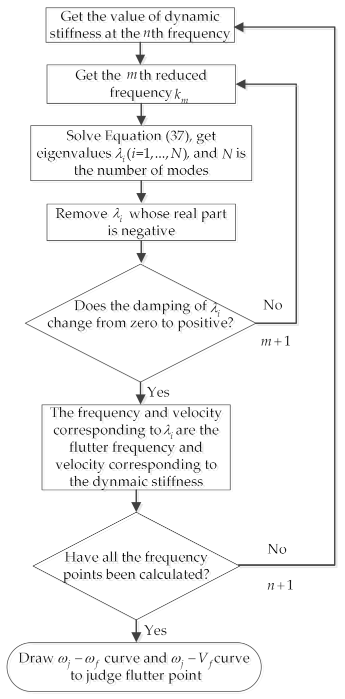
4.1.2. Flutter Analysis with V–g Method

Using dynamic stiffness to conduct the frequency-domain flutter analysis. The force in Equation (1) is the aerodynamic force in Equation (2), and ignoring $C$ yields:

$$(-{\omega }^{2}M+K)x=q_{\infty }Ax$$

(18)

The generalized stiffness matrix $K$ is a complex matrix due to the dynamic stiffness. Therefore, the equation above using the V–g method [54] is:

$$[-{\omega }^{2}M+(1+ig)K(\omega )]x=q_{\infty }Ax$$

(19)

where $ig$ is the added artificial complex structural damping.

Let the eigenvalue of Equation (19) be $\lambda ={\omega }^2/(1+ig)$, and substituting $\lambda$ and $k=\omega b/V$ into Equation (19) yields:

$$K(\omega )x=\lambda (M+\frac{\rho b^2}{2k^2})Ax$$

(20)

In Equation (20), both $k$ and $K(\omega )$ are related to the oscillation frequency $\omega$. Therefore, an iterative solution is required for this eigenvalue problem (see Figure 11).

4.2. Time Domain Method

The whole time domain mathematical fin–actuator model was integrated into SIMULINK, and the in-built “ode23s” was used for numerical simulation. When the time domain simulation starts, release the fin from an initial angular position, then change the flight speed, and the angular position response of the fin can be seen. Flutter has occurred when the oscillation is diverging. The fin may maintain a certain angle of oscillation with constant frequency before large-angle divergence occurs. This phenomenon is called LCO. Although the time domain method is time-consuming for nonlinear problems, the results are more accurate than the frequency domain method. Therefore, the subsequent analysis mainly focuses on the time domain. The frequency domain is used as a comparative verification.

5. Aeroelastic Analysis Results and Discussion

In this article, the impact of the actuator structural nonlinearities such as freeplay and friction on the fin–actuator aeroelastic characteristics were studied, and other nonlinearities were excluded.

5.1. Identification of Actuator Parameters

The actuator parameters are listed in

Table 3. Simulation parameters of the actuator. Electromotive force, EMF.

Description	Symbol	Value	Unit
Inductance	$L$	$6.53\times {10}^{-4}$	mH
Resistance	$R$	1.1	$\mathsf{\Omega }$
Rotor inertia	$J_{\mathrm{m}}$	$1.094\times {10}^{-6}$	$\mathrm{kg}\cdot {\mathrm{m}}^2$
Torque coefficient	$K_{\mathrm{m}}$	0.0238	Nm/A
Back EMF coefficient	$C_{\mathrm{e}}$	0.034	V/(rad/s)
Connection stiffness	$k_{\mathrm{m}}$	1000	Nm/rad
Moment of inertia of gear 1	$J_1$	$2.4\times {10}^{-8}$	$\mathrm{kg}\cdot {\mathrm{m}}^2$
Radius of gear 1	$r_1$	0.005	m
Moment of inertia of gear 2	$J_2$	$4\times {10}^{-6}$	$\mathrm{kg}\cdot {\mathrm{m}}^2$
Radius of gear 2	$r_2$	0.0225	m
Meshing stiffness	$k_{\mathrm{g}}$	${10}^8$	$\mathrm{kg}\cdot {\mathrm{s}}^2/\mathrm{rad}$
Connection stiffness	$k_{\mathrm{z}}$	1000	Nm/rad
Screw inertia	$J_{\mathrm{sg}}$	$3.98\times {10}^{-5}$	$\mathrm{kg}\cdot {\mathrm{m}}^2$
Radius of screw	$r_{sg}$	0.006	m
Screw efficiency	$\eta$	0.85
Fork length	$L_{\mathrm{bc}}$	0.0285	m
Comprehensive stiffness	$k_{\mathrm{c}}$	$2.27\times {10}^6$	${\mathrm{kg}/\mathrm{s}}^2$
Bristle stiffness	${\sigma }_0$	300	Nm/rad
Bristle damping	${\sigma }_1$	2.5	Nm/(rad/s)
Viscous damping	${\sigma }_2$	0.02	Nm/(rad/s)
Coulomb friction	$F_{\mathrm{c}}$	1.2565	Nm
Maximum static friction force	$F_{\mathrm{s}}$	0.774	Nm
Stribeck velocity	$V_{\mathrm{s}}$	1	rad/s

. The parameters of the friction model are identified according to the method in Reference [41]. Several constant velocity experiments were carried out to obtain the static parameters of the model. The dynamic parameters are obtained during the pre-sliding process.

5.2. Preliminary Flutter Results for No-Freeplay Gap ($e=0$) and No-Friction

The fin was released from the initial fin shaft deflection angle of 1°. Figure 12 shows the time domain response of the fin under aerodynamic force. Comparison has been made between the responses of the fin shaft angle at two flight velocities. Flutter occurred at 765 m/s, and when the flight velocity was lower than 765 m/s, the fin shaft angle response was convergent.

The flutter results in frequency domain are shown in Figure 13. Eighty-two frequency points were selected from 40 Hz to 120 Hz. The corresponding dynamic stiffness was adopted to obtain the flutter frequency and velocity of the system at each frequency point. Then a line was drawn with slope 1 that indicated the frequencies of abscissa and ordinate were equal. The frequency corresponding to the intersection of the flutter frequency line and the line with slope 1 was the real flutter frequency, which was 55.1077 Hz. The velocity corresponding to the real flutter frequency was the real flutter velocity, which was 769.2596 m/s. The frequency-domain and time-domain results were in good agreement; the discrepancy between which was of the order of 0.5%. This result shows that the calculation method of dynamic stiffness was correct and the flutter result of fin–actuator system calculated using dynamic stiffness was accurate enough.

5.3. Aeroelastic Characteristics of the Fin–Actuator System with Freeplay

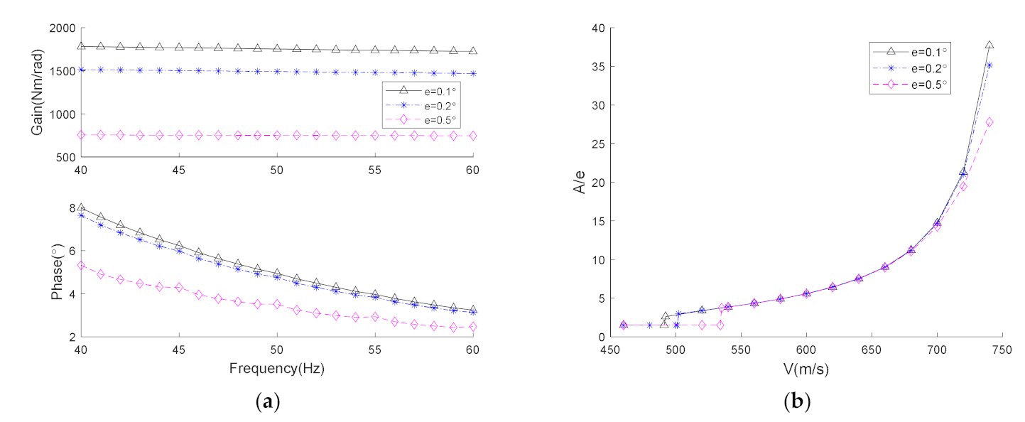
5.3.1. Influence of Different Initial Deflection Angle with $e={0.2}^{\circ }$

The initial conditions will affect the stability of nonlinear systems. The half width of freeplay at the fin shaft was 0.2°, and the initial fin shaft deflection angles ${\delta }_0$ were 0.5°, 1°, and 2°, respectively. The corresponding actuator dynamic stiffness under different ${\delta }_0$ was calculated, and the results are shown in Figure 14.

It can be discovered from Figure 14a that as ${\delta }_0$ increases, the gain of the dynamic stiffness also increased greatly, but it was not proportional to the increase in ${\delta }_0$, and the increase in phase was very small. In Reference [55], the actuator dynamic stiffness was obtained by experiments and simulations in a series of cases including changing the initial preload. The conclusion was consistent with the change of the initial angle in this paper. However, flutter analysis was not carried out in Reference [55]. Actually, ${\delta }_0$ will also affect the aeroelastic characteristics of the system, which can be seen in Figure 15b. ${\delta }_0$ will affect the speed at which the fin begins to oscillate. As ${\delta }_0$ increases, the oscillation occurs at smaller flight speed, and the oscillation amplitude becomes larger. However, different ${\delta }_0$ have little effect on $A/e$—namely, the ratio of oscillation amplitude of the fin to the width of freeplay at the same flight speed. It only has some influence on $A/e$ at the beginning of oscillation.

When ${\delta }_0$ is 1°, the comparison of the frequency domain and time domain results is shown in Figure 15, which shows that these results were highly consistent and the maximum error did not exceed 1.2%. As the flight speed increased, the oscillation amplitude suddenly increased at a certain speed, which means that flutter occurred. The oscillation frequency increased slowly within a small range with the increase in flight speed.

5.3.2. Influence of Different Freeplay with ${\delta }_0=1^{\circ }$

Keep ${\delta }_0$ at 1° and change the freeplay. When the half-widths of freeplay are 0.1°, 0.2°, and 0.5°, calculate the corresponding actuator dynamic stiffness as shown in Figure 16.

The experimental results in Reference [55] showed that the dynamic stiffness of the actuator with a smaller freeplay gap will reach a larger value. What is not mentioned in the conclusion of Reference [55] is that the phase was not affected much by the freeplay gap, although it can be seen from the experimental results. Freeplay is symmetrical nonlinearity; thus, the phase of its describing function was zero. Figure 16a also confirms that the smaller the freeplay is, the larger the amplitude is, while the phase changes little.

Figure 16b shows the time domain results of aeroelastic analysis. The torsional response amplitude increases as the flight velocity increases, and the oscillation amplitude increases as the width of freeplay increases, which are mentioned in Reference [56] too. Moreover, different widths of freeplay also have an influence on the velocity at which the fin begins to oscillate. It should be noted that the ratio of oscillation amplitude of the fin to $e$ was almost not affected by $e$ just after reaching the oscillating velocity. However, as the flight speed increased, the smaller the freeplay width, the larger the ratio.

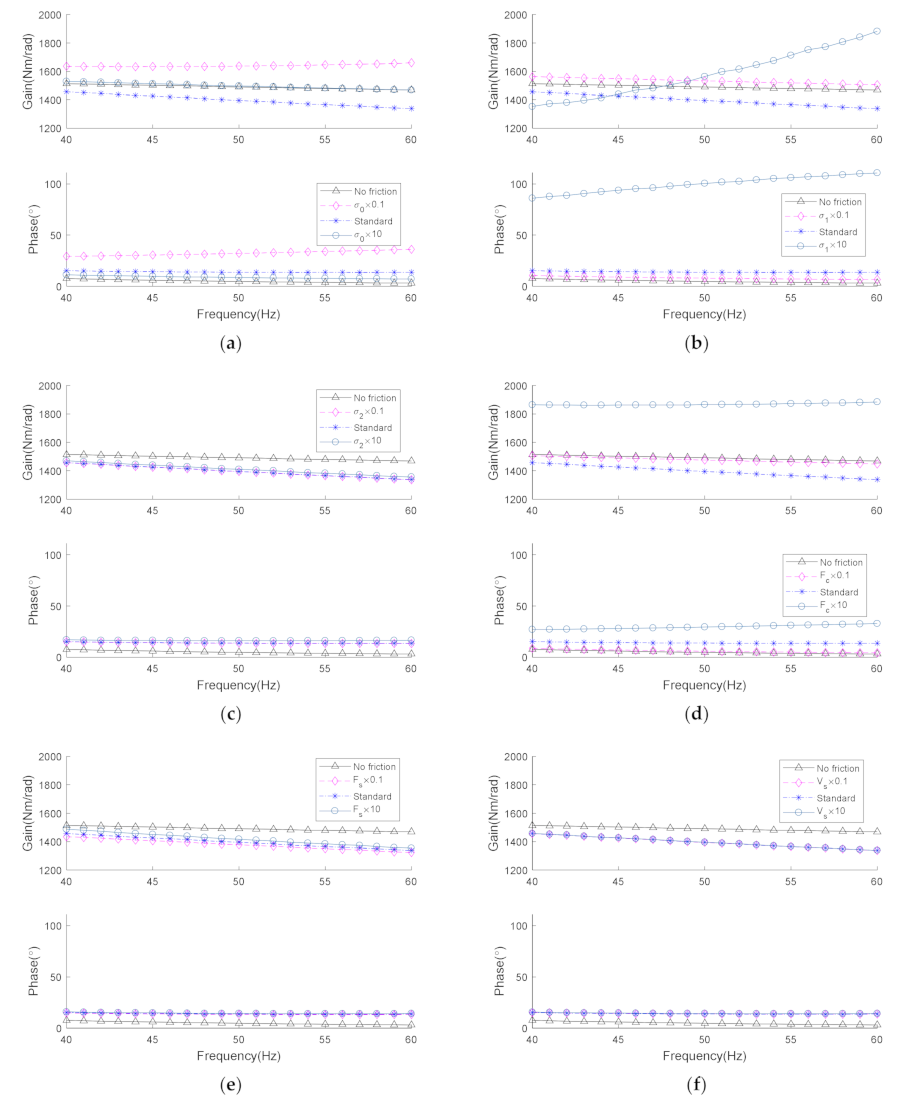
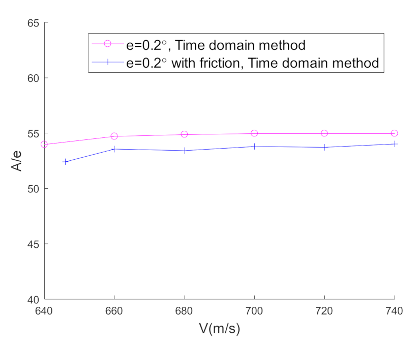
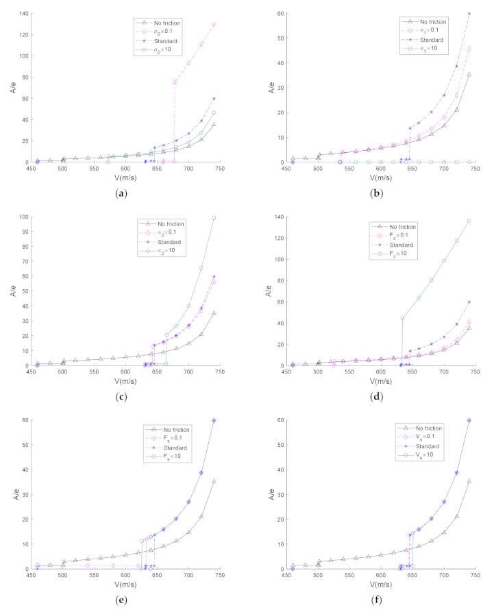
5.4. Aeroelastic Characteristics of the System with Freeplay and Friction

The LuGre model is represented by several nonlinear functional equations, including six parameters in which ${\sigma }_0$ and ${\sigma }_1$ are two dynamic parameters, and ${\sigma }_2$, $F_{\mathrm{c}}$, $F_{\mathrm{s}}$, and $V_{\mathrm{s}}$ are four static parameters. Analyzing the effect of friction on the flutter characteristics is challenging since coupling exists among the six parameters [57,58]. However, it is undoubtedly an effective way to analyze the aeroelastic characteristics with the help of the concept of dynamic stiffness and the physical meaning of the parameters. ${\sigma }_0$ and ${\sigma }_1$ are related to material properties. If a lubricant exists, ${\sigma }_2$ indicates the viscous properties of the lubricant. For dry friction, ${\sigma }_2$ is pretty small and close to zero [26]. The pressure influences on $F_{\mathrm{s}}$, $F_{\mathrm{c}}$, and $V_{\mathrm{s}}$ [59]. The variable–parameter analysis is conducted to evaluate the influence of each parameter.

Table 4. Approximate ranges and influence factors for the parameters of the LuGre model.

Description	Symbol	PARAMETER RANGE	Unit	Parameter Depends Principally upon [26,59,63]
Bristle stiffness	${\sigma }_0$	$10.23\text{~}6.5\times {10}^4$	Nm/rad	Material properties
Bristle damping	${\sigma }_1$	$2.719\times {10}^{-3}$~45.2	Nm/(rad/s)	Contact geometry and lubricant
Viscous damping	${\sigma }_2$	$9.216\times {10}^{-6}$~1.819	Nm/(rad/s)	Lubricant
Coulomb friction	$F_{\mathrm{c}}$	$1.895\times {10}^{-3}$~2646.856	Nm	Lubricant, contact geometry, and pressure
Maximum static friction force	$F_{\mathrm{s}}$	$3.124\times {10}^{-3}$~8.558	Nm	Boundary lubrication and pressure
Stribeck velocity	$V_{\mathrm{s}}$	$6.109\times {10}^{-2}$~88.1	rad/s	Lubricant and pressure

summarizes the range of friction parameters and the factors that parameter depends principally upon. As can be seen, lubricant is an important factor, but there is no lubricant added to the friction sheet of the actuator generally. Since the LuGre parameters depend on the material properties and working conditions, when the parameters are changed for stability analysis, they cannot be divorced from reality. Here, the upper and lower bounds of the parameters were derived from the literature [26,41,60,61,62]. For comparison, the standard value of each friction parameter in Table 3 was multiplied by factors of 0.1 and 10, after which the parameter values were still in the range of Table 4.

Figure 17 shows the impact of the variation of six friction parameters on the actuator dynamic stiffness when ${\delta }_0$ is 1° and $e$ is 0.2°. It was discovered that changing ${\sigma }_2$, $F_{\mathrm{s}}$, or $V_{\mathrm{s}}$ had little effect on the dynamic stiffness, while changes in ${\sigma }_0$, ${\sigma }_1$, and $F_{\mathrm{c}}$ had a greater effect. It can be observed that, generally, friction had a huge influence on both gain and phase of actuator dynamic stiffness. This is because the friction model used in this paper is complex and highly nonlinear. Friction has been oversimplified in some literatures. The actuator in Reference [64] was equivalent to a spring with friction nonlinearity, and the relationship between displacement and restoring force is given by:

$$F(x)=\left\{\begin{array}{c}Kx+F_f\begin{array}{c}at\begin{array}{c}x>0\end{array}\end{array}\\ Kx-F_f\begin{array}{c}at\begin{array}{c}x<0\end{array}\end{array}\end{array}\right.$$

(21)

The equivalent stiffness of this nonlinear spring is calculated by the describing function method. The results in Reference [64] show that friction only affects the amplitude of actuator stiffness, which has been modified in this paper according to Figure 17.

Figure 18 shows the comparison of the frequency-domain and time-domain results. The friction parameters are standard values in Table 3 and keep $e$ at 0.2°. Due to the nonlinearity of the friction model, as the oscillation amplitude increased, the difference between the time-domain and frequency-domain results became larger, but it did not exceed 4.4%. The oscillation frequency increased slightly as the flight speed increased. It is mentioned in Reference [21] that adding friction makes the frequency of LCO decrease slightly. Figure 19 compares time-domain frequencies in Figure 15b and Figure 18b, which confirms this conclusion.

Figure 20 shows the time-domain results, which also confirm that the six parameters had different effects on the system’s stability.

In Figure 20, we can draw a conclusion that $F_{\mathrm{s}}$ and $V_{\mathrm{s}}$ have little influence on the aeroelastic characteristics. This corresponds to the fact that they have little effect on dynamic stiffness. As $F_{\mathrm{s}}$ increases, the flight speed at which the fin begins to oscillate first increases and then decreases slightly, while the oscillation amplitude at the same flight speed remains almost unchanged. As $V_{\mathrm{s}}$ increases, the flight speed at which the fin begins to oscillate also increases slightly, while the oscillation amplitude at the same flight speed is almost unchanged.

${\sigma }_1$ seems to be the parameter that has the greatest influence on the aeroelastic characteristics in the variable–parameter analysis. It can be seen that increasing ${\sigma }_1$ can greatly improve the stability of the system. When ${\sigma }_1$ is 10 times the standard value, the fin deflection angle always converges within the flight speed range of interest. This parameter is difficult to quantify in actual engineering. It can be increased by changing the contact surface geometry, that is, increasing the roughness of the contact surface. More work is needed to quantify and standardize ${\sigma }_1$ in the future.

$F_{\mathrm{c}}$, which stands for Coulomb friction, can be studied as a separate friction model. Compared with what is mentioned in Reference [20]—that increasing the maximum friction torque of Coulomb friction can increase the flutter speed and reduce the amplitude of the pitch response—we discover that the influence of $F_{\mathrm{c}}$ on system stability is complicated. As $F_{\mathrm{c}}$ increases, the speed at which the fin starts to oscillate first increases and then decreases, while the oscillation amplitude at the same flight speed increases. Therefore, $F_{\mathrm{c}}$ is not the larger the better. An optimal $F_{\mathrm{c}}$ can be obtained by appropriately designing the lubrication, pressure, and the geometry of the contact surface between the friction sheet and fork, so that the system is stable and friction is reduced.

In addition to ${\sigma }_1$ and $F_{\mathrm{c}}$, ${\sigma }_0$ and ${\sigma }_2$ also have a non-negligible effect on the aeroelastic characteristics. The smaller the ${\sigma }_0$, the greater the flight speed at which the fin starts to oscillate, which is the desired effect. However, once the oscillation starts in this case, the amplitude will increase sharply. As mentioned earlier, ${\sigma }_2$ is related to lubricants, so it is not the focus of this study. It can be seen that larger ${\sigma }_2$ will slightly increase the speed at which the fin starts to oscillate, but it will also cause the amplitude of oscillation to increase at the same flight speed.

As mentioned earlier, a large number of studies have used the Coulomb model. Some researchers have discovered the limitations of Coulomb friction. They have noticed that with the increase of friction, the stable region increased, but the stable boundary changed little [19]. Wayhs-Lopes et al. studied the effects of both freeplay and Coulomb friction last year, pointed out that although friction is dissipative, it is not enough to restrain LCO [21]. However, the analysis in this article is sufficient to show that a single factor may have limitations. The synergistic effect of multiple parameters can suppress the LCO in the low-speed range, and it is also effective in increasing the flutter velocity and reducing the oscillation amplitude.

6. Conclusions

In this article, a high-fidelity model of a fin–actuator system with a typical configuration was established based on modularization, in which a friction sheet was modeled utilizing the LuGre model, which can better reflect the friction characteristics. The whole modeling method can be used for dynamic analysis and aeroelastic analysis.

The aeroelastic characteristics of the system were analyzed using frequency-domain and time-domain methods. The results of the two methods were highly consistent. The time-domain method can deal with highly nonlinear situations, while the frequency-domain method based on the DF method is suitable for weak nonlinear systems.

Initial conditions, freeplay, and friction will all affect the stability of the nonlinear system. As the initial deflection angle ${\delta }_0$ increases, the gain of the dynamic stiffness will be larger, but the increase was not proportional, and the increase of the phase was minor. The oscillation occurred at smaller flight speed, and the oscillation amplitude $A$ became larger. Different ${\delta }_0$ have little effect on the ratio of $A$ to the half width of freeplay $e$ at the same flight speed. Dynamic stiffness of the actuator with a smaller freeplay gap will reach a larger value, while the phase was not affected much by freeplay gap. The oscillation amplitude increased as the width of freeplay increased.

Friction affects the amplitude and phase of actuator dynamic stiffness greatly. Adding friction makes the frequency of LCO decrease slightly. The LuGre friction model has six parameters. Friction sheets that do not use lubricant, ${\sigma }_2$, which reflects the viscosity of the lubricant, were not the focus of this study. $F_{\mathrm{s}}$ and $V_{\mathrm{s}}$ have little influence on the aeroelastic characteristics, which corresponds to the fact that they have little effect on dynamic stiffness. ${\sigma }_1$ is the parameter that has the greatest influence on the aeroelastic characteristics. Increasing ${\sigma }_1$ can greatly improve the stability of the system. However, ${\sigma }_1$ is difficult to quantify in actual engineering. The influence of $F_{\mathrm{c}}$ on system stability is complicated. As $F_{\mathrm{c}}$ increased, the speed at which the fin started to oscillate first increased and then decreased, while the oscillation amplitude at the same flight speed increased. Therefore, $F_{\mathrm{c}}$ was not better when larger. An optimal $F_{\mathrm{c}}$ can be obtained by appropriately designing the lubrication, pressure, and the geometry of the contact surface between the friction sheet and fork, so that the system is stable and friction is reduced. The smaller the ${\sigma }_0$, the greater the flight speed at which the fin starts to oscillate, which was the desired effect. However, once the oscillation started in this case, the amplitude increased sharply. A single factor may have limitations. The synergistic effect of multiple parameters can suppress the LCO in the low-speed range, and it is also effective in increasing the flutter velocity as well as reducing the oscillation amplitude.

References

1. Librescu, L.; Marzocca, P. Advances in the Linear/Nonlinear Control of Aeroelastic Structural Systems. Acta Mech. 2005, 178, 147–186. [Google Scholar] [CrossRef]
2. Karpel, M. Design for Active and Passive Flutter Suppression and Gust Alleviation. Ph.D. Thesis, Stanford University, Stanford, CA, USA, 1981. [Google Scholar]
3. Yoo, C.-H.; Lee, Y.-C.; Lee, S.-Y. A Robust Controller for an Electro-Mechanical Fin Actuator. In Proceedings of the 2004 American Control Conference, Boston, MA, USA, 30 June–2 July 2004; Volume 5, pp. 4010–4015. [Google Scholar]
4. Kim, S.H.; Tahk, M.-J. Dynamic Stiffness Transfer Function of an Electromechanical Actuator Using System Identification. Int. J. Aeronaut. Space Sci. 2018, 19, 208–216. [Google Scholar] [CrossRef]
5. Yehezkely, E.; Karpel, M. Nonlinear Flutter Analysis of Missiles with Pneumatic Fin Actuators. J. Guid. Control Dyn. 1996, 19, 664–670. [Google Scholar] [CrossRef]
6. Shin, W.-H.; Lee, I.; Shin, Y.-S.; Bae, J.-S. Nonlinear Aeroelastic Analysis for a Control Fin with an Actuator. J. Aircr. 2007, 44, 597–605. [Google Scholar] [CrossRef]
7. Yang, N.; Wu, Z.; Yang, C. Structural Nonlinear Flutter Characteristics Analysis for an Actuator-Fin System with Dynamic Stiffness. Chin. J. Aeronaut. 2011, 24, 590–599. [Google Scholar] [CrossRef] [Green Version]
8. Paek, S.-K.; Lee, I. Flutter Analysis for Control Surface of Launch Vehicle with Dynamic Stiffness. Comput. Struct. 1996, 60, 593–599. [Google Scholar] [CrossRef]
9. Shin, W.-H.; Lee, S.-J.; Lee, I.; Bae, J.-S. Effects of Actuator Nonlinearity on Aeroelastic Characteristics of a Control Fin. J. Fluids Struct. 2007, 23, 1093–1105. [Google Scholar] [CrossRef]
10. Zhang, R.; Wu, Z.; Yang, C. Dynamic Stiffness Testing-Based Flutter Analysis of a Fin with an Actuator. Chin. J. Aeronaut. 2015, 28, 1400–1407. [Google Scholar] [CrossRef] [Green Version]
11. Zhang, P.; Zhang, K.; Shen, Y. Research on Nonlinear Mechanical Properties for Actuator Structure. Aero Weapon. 2015, 3, 38–43. [Google Scholar]
12. Kingsbury, D.W.; Agelastos, A.M.; Dietz, G.; Mignolet, M.; Liu, D.D.; Schewe, G. Limit Cycle Oscillations of Aeroelastic Systems with Internal Friction in the Transonic Domain—Experimental Results. In Proceedings of the 46th AIAA/ASME/ASCE/AHS/ASC Structures, Structural Dynamics and Materials Conference, Austin, TX, USA, 18–21 April 2005; Volume 2, pp. 1412–1422. [Google Scholar]
13. Ravanbod-Shirazi, L.; Besancon-Voda, A. Friction Identification Using the Karnopp Model, Applied to an Electropneumatic Actuator. Proc. Inst. Mech. Eng. Part I J. Syst. Control Eng. 2003, 271, 123–138. [Google Scholar] [CrossRef]
14. Torkaman, A. Flutter Stability of Shrouded Turbomachinery Cascades with Nonlinear Frictional Damping. Electronic Theses and Dissertations, 2004–2019. 2018. Available online: https://stars.library.ucf.edu/etd/6169/ (accessed on 14 January 2019).
15. Khalak, A. A Framework for Flutter Clearance of Aeroengine Blades. J. Eng. Gas Turbines Power 2002, 124, 1003–1010. [Google Scholar] [CrossRef]
16. Griffin, J.H. Friction Damping of Resonant Stresses in Gas Turbine Engine Airfoils. J. Eng. Power 1980, 102, 329–333. [Google Scholar] [CrossRef]
17. Whiteman, W.E.; Ferri, A.A. Suppression of Bending-Torsion Flutter through Displacement-Dependent Dry Friction Damping. AIAA J. 1999, 31, 79–83. [Google Scholar] [CrossRef]
18. Mignolet, M.; Agelastos, A.; Liu, D. Impact of Frictional Structural Nonlinearity in the Presence of Negative Aerodynamic Damping. In Proceedings of the 44th AIAA/ASME/ASCE/AHS/ASC Structures, Structural Dynamics, and Materials Conference, Norfolk, VA, USA, 7–10 April 2003; p. 1428. [Google Scholar]
19. Tan, T.; Li, M.; Liu, B. Stability Analysis of an Aeroelastic System with Friction. Chin. J. Aeronaut. 2013, 26, 624–630. [Google Scholar] [CrossRef] [Green Version]
20. Lu, L.; Li, M.; Gan, K. Influence of Coulomb Friction on Two-Dimensional Aeroelastic Airfoils. Eng. Mech. 2015, 5, 250–256. [Google Scholar]
21. Wayhs-Lopes, L.D.; Dowell, E.H.; Bueno, D.D. Influence of Friction and Asymmetric Freeplay on the Limit Cycle Oscillation in Aeroelastic System: An Extended Hénon’s Technique to Temporal Integration. J. Fluids Struct. 2020, 96, 103054. [Google Scholar] [CrossRef]
22. Sang, Y.; Gao, H.; Xiang, F. Practical Friction Models and Friction Compensation in High-Precision Electro-Hydraulic Servo Force Control Systems. Instrum. Sci. Technol. 2014, 42, 184–199. [Google Scholar] [CrossRef]
23. Dahl, P.R. Measurement of Solid Friction Parameters of Ball Bearings; Aerospace Corp El Segundo Ca Engineering Science Operations: El Segundo, CA, USA, 1977. [Google Scholar]
24. De Wit, C.C.; Olsson, H.; Astrom, K.J.; Lischinsky, P. A New Model for Control of Systems with Friction. IEEE Trans. Autom. Control 1995, 40, 419–425. [Google Scholar] [CrossRef] [Green Version]
25. De Wit, C.C.; Lischinsky, P. Adaptive Friction Compensation with Partially Known Dynamic Friction Model. Int. J. Adapt. Control Signal Process. 1997, 11, 65–80. [Google Scholar] [CrossRef]
26. Swevers, J.; Al-Bender, F.; Ganseman, C.G.; Projogo, T. An Integrated Friction Model Structure with Improved Presliding Behavior for Accurate Friction Compensation. IEEE Trans. Autom. Control 2000, 45, 675–686. [Google Scholar] [CrossRef]
27. Lampaert, V.; Swevers, J.; Al-Bender, F. Modification of the Leuven Integrated Friction Model Structure. IEEE Trans. Autom. Control 2002, 47, 683–687. [Google Scholar] [CrossRef] [Green Version]
28. Lampaert, V.; Al-Bender, F.; Swevers, J. A Generalized Maxwell-Slip Friction Model Appropriate for Control Purposes. In Proceedings of the 2003 IEEE International Workshop on Workload Characterization (IEEE Cat. No. 03EX775), Saint Petersburg, Russia, 20–22 August 2003; Volume 4, pp. 1170–1177. [Google Scholar]
29. Al-Bender, F.; Lampaert, V.; Swevers, J. The Generalized Maxwell-Slip Model: A Novel Model for Friction Simulation and Compensation. IEEE Trans. Autom. Control 2005, 50, 1883–1887. [Google Scholar] [CrossRef]
30. Ruderman, M.; Bertram, T. Two-State Dynamic Friction Model with Elasto-Plasticity. Mech. Syst. Signal Process 2013, 39, 316–332. [Google Scholar] [CrossRef]
31. Wang, X.; Wang, S. High Performance Adaptive Control of Mechanical Servo System with LuGre Friction Model: Identification and Compensation. J. Dyn. Syst. Meas. Control 2012, 134, 011021. [Google Scholar] [CrossRef] [Green Version]
32. Mate, C.M.; Carpick, R.W. Tribology on the Small Scale: A Modern Textbook on Friction, Lubrication, and Wear; Oxford University Press: New York, NY, USA, 2019. [Google Scholar]
33. Tustin, A. The Effects of Backlash and of Speed-Dependent Friction on the Stability of Closed-Cycle Control Systems. J. Inst. Electr. Eng. Part IIA Autom. Regul. Servo Mech. 1947, 94, 143–151. [Google Scholar] [CrossRef]
34. Osborne, N.; Rittenhouse, D. The Modeling of Friction and Its Effects on Fine Pointing Control. In Proceedings of the Mechanics and Control of Flight Conference, Anaheim, CA, USA, 5–9 August 1974; p. 875. [Google Scholar]
35. Li, L.; Wang, F.Y.; Zhou, Q. Integrated Longitudinal and Lateral Tire/Road Friction Modeling and Monitoring for Vehicle Motion Control. IEEE Trans. Intell. Transp. Syst. 2006, 7, 1–19. [Google Scholar] [CrossRef]
36. Brandenburg, G.; Schafer, U. Influence and Compensation of Coulomb Friction in Industrial Pointing and Tracking Systems. In Proceedings of the Conference Record of the 1991 IEEE Industry Applications Society Annual Meeting, Dearborn, MI, USA, 28 September–4 October 1991; pp. 1407–1413. [Google Scholar]
37. Olsson, H.; Astrom, K.J. Friction Generated Limit Cycles. IEEE Trans. Control Syst. Technol. 2001, 9, 629–636. [Google Scholar] [CrossRef] [Green Version]
38. Canudas, C.; Astrom, K.; Braun, K. Adaptive Friction Compensation in DC-Motor Drives. IEEE Robot Autom. Mag. 1987, 3, 681–685. [Google Scholar] [CrossRef] [Green Version]
39. De Wit, C.C. Robust Control for Servo-Mechanisms under Inexact Friction Compensation. Automatica 1993, 29, 757–761. [Google Scholar] [CrossRef]
40. Giorgio, I.; Del Vescovo, D. Energy-based trajectory tracking and vibration control for multilink highly flexible manipulators. Math. Mech. Complex Syst. 2019, 7, 159–174. [Google Scholar] [CrossRef] [Green Version]
41. Wang, X.; Lin, S.; Wang, S. Dynamic Friction Parameter Identification Method with Lugre Model for Direct-Drive Rotary Torque Motor. Math. Probl. Eng. 2016, 2016, 6929457. [Google Scholar] [CrossRef] [Green Version]
42. Feyel, P.; Duc, G.; Sandou, G. LuGre Friction Model Identification and Compensator Tuning Using a Differential Evolution Algorithm. In Proceedings of the 2013 IEEE Symposium on Differential Evolution (SDE), Singapore, 16–19 April 2013; pp. 85–91. [Google Scholar]
43. Zhuo, G.; Wang, J.; Zhang, F. Parameter Identification of Tire Model Based on Improved Particle Swarm Optimization Algorithm; SAE Technical Paper; SAE International: Warrendale, PA, USA, 2015. [Google Scholar]
44. Saha, A.; Wiercigroch, M.; Jankowski, K.; Wahi, P.; Stefański, A. Investigation of Two Different Friction Models from the Perspective of Friction-Induced Vibrations. Tribol. Int. 2015, 90, 185–197. [Google Scholar] [CrossRef]
45. Gladwell, G.M.L. Branch Mode Analysis of Vibrating Systems. J. Sound Vib. 1964, 1, 41–59. [Google Scholar] [CrossRef]
46. Wang, W.L. Vibration and Dynamic Sub-Structure Method; Fudan University Press: Shanghai, China, 1985. [Google Scholar]
47. Piccardo, G. A Methodology for the Study of Coupled Aeroelastic Phenomena. J. Wind. Eng. Ind. Aerodyn. 1993, 48, 241–252. [Google Scholar] [CrossRef]
48. Version 9.3. Theoretical Manual, ZONA Technology. 2017. Available online: https://www.zonatech.com/downloads.html#ProductDocumentation (accessed on 14 January 2019).
49. Astrom, K.J.; De Wit, C.C. Revisiting the Lugre Model Stick-Slip Motion and Rate Dependence. IEEE Control Syst. 2008, 28, 101–114. [Google Scholar]
50. Liu, J. MATLAB Simulation of Advanced PID Control, 2nd ed.; Electronic Industry Press: Beijing, China, 2004. [Google Scholar]
51. Krylov, N.M.; Bogoliubov, N. Introduction to Nonlinear Mechanics; Princeton University Press: Princeton, NJ, USA, 1943. [Google Scholar]
52. Blaquiere, A. Nonlinear System Analysis; Elsevier: Amsterdam, The Netherlands, 2012. [Google Scholar]
53. Kochenburger, R.J. A Frequency Response Method for Analyzing and Synthesizing Contactor Servomechanisms. Trans. Am. Inst. Electr. Eng. 1950, 69, 270–284. [Google Scholar] [CrossRef]
54. Wright, J.R.; Cooper, J.E. Introduction to Aircraft Aeroelasticity and Loads; John Wiley & Sons: Hoboken, NJ, USA, 2008. [Google Scholar]
55. Kim, S.H.; Tahk, M.J. Modeling and Experimental Study on the Dynamic Stiffness of an Electromechanical Actuator. J. Spacecr. Rocket. 2016, 53, 708–719. [Google Scholar] [CrossRef]
56. Tang, D.; Dowell, E.H. Aeroelastic Response Induced by Free Play, Part 1: Theory. AIAA J. 2011, 49, 2532–2542. [Google Scholar] [CrossRef]
57. Hensen, R.H.; van de Molengraft, M.J.; Steinbuch, M. Frequency Domain Identification of Dynamic Friction Model Parameters. IEEE Trans. Control Syst. Technol. 2002, 10, 191–196. [Google Scholar] [CrossRef]
58. Rizos, D.D.; Fassois, S.D. Friction Identification Based upon the LuGre and Maxwell Slip Models. IEEE Trans. Control Syst. Technol. 2008, 17, 153–160. [Google Scholar] [CrossRef]
59. Tran, X.B.; Yanada, H. Dynamic Friction Characteristics of Pneumatic Actuators and Their Mathematical Model. In Proceedings of the 8th JFPS International Symposium on Fluid Power, Okinawa, Japan, 25–28 October 2011; pp. 657–664. [Google Scholar]
60. Xiao, Q.; Jia, H.; Zhang, J.; Han, X.; Xi, R. Identification and Compensation of Nonlinearity for Electromechanical Actuator Servo System. Opt. Precis. Eng. 2013, 21, 2038–2047. [Google Scholar] [CrossRef]
61. Yu, W.; Ma, J.; Li, J.; Xiao, J. Friction Parameter Identification and Friction Compensation for Precision Servo Turning Table. Opt. Precis. Eng. 2011, 19, 2736–2743. [Google Scholar] [CrossRef]
62. Liu, Q.; Hu, H.; Liu, J.; Er, L. Research on the Parameter Identification of Friction Model for Servo Systems Based on Genetic Algorithms. J. Syst. Eng. Electron. 2003, 77–79. [Google Scholar]
63. Armstrong-Hélouvry, B.; Dupont, P.; De Wit, C.C. A Survey of Models, Analysis Tools and Compensation Methods for the Control of Machines with Friction. Automatica 1994, 30, 1083–1138. [Google Scholar] [CrossRef]
64. Lee, S.J.; Lee, I.; Shin, W.H. Flutter Characteristics of Aircraft Wing Considering Control Surface and Actuator Dynamics with Friction Nonlinearity. Int. J. Aeronaut. Space Sci. 2007, 8, 140–147. [Google Scholar] [CrossRef]
65. Zhang, X.; Wu, Z.; Yang, C. New Flutter-Suppression Method for a Missile Fin with an Actuator. J. Aircraft 2013, 50, 989–994. [Google Scholar] [CrossRef]
66. Karpel, M. Design for Active Flutter Suppression and Gust Alleviation Using State-Space Aeroelastic Modeling. J. Aircraft 1982, 19, 221–227. [Google Scholar] [CrossRef]
Figure 1. Model comparison for flutter analysis, where (a) is the model of the conventional fin–actuator system and (b) is the fin–actuator system considering the characteristics of an actuator.
Applsci 11 03057 g001
Figure 2. Schematic representation of the LuGre friction model.
Applsci 11 03057 g002
Figure 3. Schematic diagram of the fin–actuator system, where (a) is the whole system structure and (b) is the schematic diagram of the friction sheet position.
Applsci 11 03057 g003
Figure 4. The modal synthesis method was used to build the structure model of the fin, where (a) is the elastic branch and (b) is the rotational rigid branch.
Applsci 11 03057 g004
Figure 5. Aerodynamic model of the fin.
Applsci 11 03057 g005
Figure 6. Force diagram of the gears.
Applsci 11 03057 g006
Figure 7. Schematic diagram of the screw–nut pair and fork model.
Applsci 11 03057 g007
Figure 8. The controller and sensor model of the actuator.
Applsci 11 03057 g008
Figure 9. Schematic diagram of the system model.
Applsci 11 03057 g009
Figure 10. Schematic diagram of the actuator dynamic stiffness model.
Applsci 11 03057 g010
Figure 11. Flow chart for calculating flutter speed and frequency using dynamic stiffness.
Applsci 11 03057 g011
Figure 12. The time domain flutter results of the system without freeplay and friction, where (a) is the response of the fin shaft angle at 760 m/s, and (b) is at 765 m/s.
Applsci 11 03057 g012
Figure 13. The frequency domain flutter results of the system without freeplay and friction.
Applsci 11 03057 g013
Figure 14. The influence of δ 0 with e = 0.2 , where (a) was the influence of δ 0 on the actuator dynamic stiffness and (b) was the influence of δ 0 on the response of the fin deflection angle at different flight speeds.
Applsci 11 03057 g014
Figure 15. Comparison of the results of the flutter analysis in the time domain and frequency domain with δ 0 = 1 and e = 0.2 , where (a) is the flight speed– A / e curve and (b) is the flight speed–oscillation frequency curve.
Applsci 11 03057 g015
Figure 16. The influence of e with δ 0 = 1 , where (a) is the influence of e on the dynamic stiffness of the actuator and (b) is the influence of e on the response of the fin deflection angle at different flight speeds.
Applsci 11 03057 g016
Figure 17. Influence of the parameters of the LuGre model on the dynamic stiffness of the actuator, where (af), respectively, show the effects of σ 0 , σ 1 , σ 2 , F c , F s , and V s .
Applsci 11 03057 g017
Figure 18. Comparison of the results of flutter analysis in time domain and frequency domain with friction, when δ 0 = 1 and e = 0.2 , where (a) is the flight speed– A / e curve and (b) is the flight speed–oscillation frequency curve.
Applsci 11 03057 g018
Figure 19. Comparison of time-domain frequencies for freeplay only and freeplay with friction.
Applsci 11 03057 g019
Figure 20. Influence of the parameters of the LuGre model on the response of the fin deflection angle at different flight speeds with δ 0 = 1 and e = 0.2 , where (af), respectively, show the effects of σ 0 , σ 1 , σ 2 , F c , F s , and V s .
Applsci 11 03057 g020