Communication

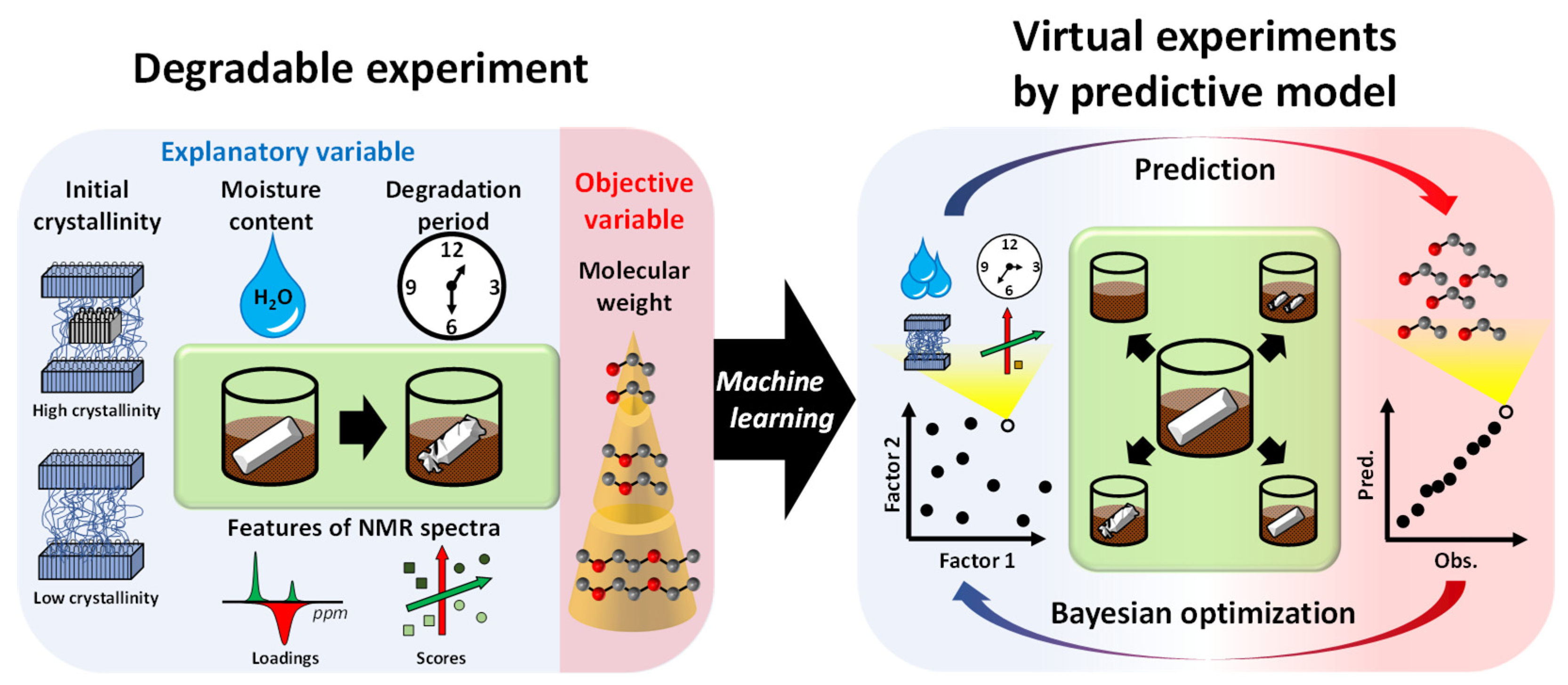
Decomposition Factor Analysis Based on Virtual Experiments throughout Bayesian Optimization for Compost-Degradable Polymers

1
Graduate School of Medical Life Science, Yokohama City University, 1-7-29 Suehiro-cho, Tsurumi-ku, Yokohama, Kanagawa 230-0045, Japan
2
RIKEN Center for Sustainable Resource Science, 1-7-22 Suehiro-cho, Tsurumi-ku, Yokohama, Kanagawa 230-0045, Japan
3
Graduate School of Bioagricultural Sciences, Nagoya University, 1 Furo-cho, Chikusa-ku, Nagoya, Aichi 464-0810, Japan
*
Author to whom correspondence should be addressed.
Appl. Sci. 2021, 11(6), 2820; https://doi.org/10.3390/app11062820
Submission received: 24 February 2021 / Revised: 15 March 2021 / Accepted: 18 March 2021 / Published: 22 March 2021
(This article belongs to the Special Issue Applications and Advancements of Spectroscopy)

Abstract

:
Bio-based polymers have been considered as an alternative to oil-based materials for their “carbon-neutral” environmentally degrative features. However, degradation is a complex system in which environmental factors and preparation conditions are involved, and the relationship between degradation and these factors/conditions has not yet been clarified. Moreover, an efficient system that addresses multiple degradation factors has not been developed for practical use. Thus, we constructed a decomposition degree predictive model to explore degradation factors based on analytical data and experimental conditions. The predictive model was constructed by machine learning using a dataset. The objective variable was the molecular weight, and the explanatory variables were the moisture content in a compost environment, degradation period, degree of crystallinity pre-experiment, and features of solid-state nuclear magnetic resonance spectra. The good accuracy of this predictive model was confirmed by statistical variables. The moisture content in the compost environment was a critical factor for considering initial degradation; specific scores revealed the contribution of degradation factors. Furthermore, the optimum decomposition degree, various analytical values, and experimental conditions were predictable when this predictive model was combined with Bayesian optimization. Information obtained from virtual experiments is expected to promote the material design and development of bio-based plastics.

1. Introduction

Plastics, which are lightweight and stable, are essential materials that support our daily lives most widely in the form of containers, such as plastic bottles and synthetic fibers. By contrast, owing to their high stability, pollution due to plastic disposal has become an apparent problem in many countries worldwide [1,2]. Furthermore, “carbon-neutral” bio-based polymers, such as polylactic acid (PLA), polybutylene succinate (PBS), and polycaprolactone (PCL), have become a focus in the era of biorefinery materials as an alternative to oil-based materials [3,4]. Here, we focused on PLA, which is one of the most common bio-based plastics. It is known that the degradation rate of PLA changes depending on the amount of moisture, temperature, and hydrogen ion concentration (pH) in the surrounding environment [5]; moreover, degradation factors are intricately entwined, including environmental factors and preparation conditions, and the relationship between degradation and these factors/conditions has not yet been clarified. The elucidation was considered to be extremely meaningful in predicting the degree of degradation. Moreover, a computational degradation predictive method could overcome the time and cost constraints to experimentally demonstrate bio-based plastic decomposition.
We considered how to comprehensively obtain the data for the sample and surrounding environment to solve the relationship between these complex systems, and data science analysis could be useful for this process [6,7,8,9,10,11]. In the measurement method, solid-state nuclear magnetic resonance (NMR) reflects both crystalline and amorphous structures in chemical shifts [12,13]; in particular, PLA emits broad signals for the amorphous component and sharp signals for the crystalline component in cross-polarization and magic angle spinning (13C-CP/MAS) spectra [14,15]. Therefore, we decided to use solid-state NMR as the analysis method. In the analysis method, we focused on Bayesian optimization. Bayesian optimization has already been used in material science [16,17,18,19] and is an effective method, particularly for complex systems such as preparation conditions, chemical composition, and microstructure. Moreover, this analysis method can be applied to a small number of experiments, as is typical of the design of experiments, and is considered suitable for the rapid prediction of the degree of degradation. Therefore, we decided to construct a degradation prediction model, mainly based on Bayesian optimization. Furthermore, because bio-based plastic degradation is also greatly affected by the surrounding environment, we decided to obtain the environmental conditions and incorporate them into the dataset. A degradation prediction model focusing on the surrounding environment is a new attempt.
In this study, we performed degradation experiments on PLA, which is the most common bio-based plastic; the results were used to construct a model that can predict the degree of degradation while considering the surrounding environment and degradation factors and their contribution rates. Furthermore, the optimum decomposition degree, various analytical values, and experimental conditions were explored using virtual experiments that combined the decomposition degree predictive model with Bayesian optimization.

2. Materials and Methods

2.1. Materials

PLA was purchased from Nature3D (http://nature3d.net/, accessed on 24 February 2021) in pellet form and, using a press molding machine (H300-01, AS ONE Corp., Osaka, Japan), sheet samples were formed from the PLA pellets to a standardized size of 10 mm × 30 mm and a thickness of 0.5 mm. Samples of different crystallinity were obtained by varying the descending temperature conditions or adding an annealing treatment. Three types of prepared samples which had different initial crystallinities, named R/N, R/A, and S/A, were used for decomposition experiments (Table S1).

2.2. Degradation Experiment

The degradation experiment was performed by burying the samples in containers filled with commercial composting tip materials along with targets for compost degradation of raw waste, which was purchased from Eco Clean Co., Ltd. (https://www.gotonet.co.jp/products/detail.php?product_id=8710491, accessed on 24 February 2021), storing them in a thermostatic chamber at 60 °C, and exposing the samples to a degradation environment that mimicked composting. In this experiment, we obtained samples after the decomposition experiment as well as information on the moisture content and decomposition period. The moisture content was calculated based on the water content in the soil (Ww) and the dry weight of the soil (Ws) according to the following equation:
Moisture content [%] = Ww / (Ww + Ws)
As a preliminary experiment, the approximate Ws used in the experiment was obtained for one sample by freeze-drying the soil in the container used for the experiment. Then, based on the weight of each sample, container, and Ws, we calculated the theoretical value of how much weight should be used to achieve the desired moisture content. Then, the total weight was periodically measured, and pure water was added to reach the theoretical value. The desired moisture content was adjusted every 48–72 h. After the experiment, the soil was freeze-dried to obtain the actual value of Ws, and the exact moisture content was calculated for each weighing day. For the decomposition degree predictive model, the averaged moisture content for all measurement days was used. The decomposition experiment was conducted for three weeks, and sample collection was performed every week. Information on the moisture content in the compost environment and decomposition time obtained from the above process was used as an index of the external environment.

2.3. Measurements of Samples

Before and after the decomposition experiment, the samples were subjected to various measurements. After the samples were collected, they were washed with water to remove the attached soil, freeze-dried, and stored in a desiccator until the amount of water adsorbed was equal to that before the decomposition experiment. The weight-loss ratio was then calculated by measuring the weight and comparing it with that before the decomposition experiment. The solid-state NMR spectra in this study were recorded using an Avance III HD-500 instrument (Bruker Corp., Billerica, MA, USA) equipped with a double-resonance 4.0 mm MAS probe operating at 500.13 MHz for 1H and 125.76 MHz for 13C. In solid-state NMR measurements, 13C-CP/MAS measurements and 1H static measurements were performed to collect data on the structural information of NMR spectra [20]. The 13C-CP/MAS spectra of PLA were recorded at an MAS frequency of 12 kHz at 299 K. In the 13C-CP/MAS measurements, the spectral width was 200 ppm, the observed points were 2048, and the number of scans was 1024. The 1H wide-line NMR spectra of PLA were recorded at an MAS frequency of 0 kHz at 299 K. In 1H static measurements, the spectral width was 400 ppm, the observed points were 32,768, and the number of scans was 32. All NMR spectra were pre-processed using TopSpin and Mnova software. The weight average molecular weight (Mw) of the sample was determined by gel permeation chromatography (GPC) analysis using LaChrom Elite system (Hitachi, Tokyo, Japan) equipment with a Shodex GPC K-805L column. Chloroform was used as the eluent, and the sample concentration was 10 mg/mL. When the measurement was taken, the column temperature was 30 °C, the sample injection volume was 50 μL, the flow velocity was 1.0 mL/min, and the relative molecular weight distribution was measured using an ultraviolet detector. Polystyrene standard was used for the calibration curve. Differential scanning calorimetry (DSC) was performed using DSC3500 Sirius (Netzsch Gerätebau GmbH, Selb, Germany). A sample of approximately 12 mg was weighed in an aluminum pan and measured at a nitrogen flow rate of 40 mL/min. The temperature was lowered from room temperature to 20 °C at 10 °C/min, stabilized for 10 min, and then raised to 200 °C at 10 °C/min. For sample exchange, the sample was kept at 200 °C for 5 min and then cooled to 25 °C at 20 °C/min. Cold crystallization enthalpy (ΔHcc) and melting enthalpy (ΔHm) were measured. Then, crystallinity was evaluated according to the following equation:
Crystallinity [%] = (ΔHcc + ΔHm) / 135
where 135 J/g is the theoretical maximum value of ΔHm [15].

2.4. Construction and Evaluation of Decomposition Degree Predictive Models

In this study, random forest (RF) [21] and extreme gradient boosting (XGBoost) [22] were used as machine learning algorithms to construct the predictive model for degradation. Mw and the weight-loss ratio were used as indicators of the degree of degradation. To construct a predictive model to estimate the degree of degradation by machine learning, Mw obtained by GPC was used as the objective variable. We constructed a decomposition degree predictive model using the weight-loss ratio as the objective variable and compared the predictive accuracy of the predictive models constructed by different machine learning algorithms. The NMR spectra were dimensionally compressed by principal component analysis (PCA) without centering and scaling the data. Explanatory variables in the dataset for machine learning were collected from features of the NMR spectra and initial crystallinity as analytical data, and the degradation period and moisture content in the compost environment were obtained as the experimental conditions. Dimensional compression was performed to overcome the cost limitation of Bayesian optimization. If there are too many variables, the number of search items increases, and the calculation cost becomes expensive. To factor the moisture content in the compost environment, the moisture weight was estimated from the total weight of the sample, and the values at each measurement were obtained and averaged. Accuracy of the decomposition degree predictive model was evaluated by the coefficient of determination (R2) and the root mean square error (RMSE) of experimental data and validation data with five-fold cross validation. The best hyperparameters in machine learning were explored using a three-grid search. In addition, the NMR spectra and experimental conditions at the optimal decomposition level were obtained by applying the proposed conditions to the predictive model and performing iterative calculations using Bayesian optimization. In addition, we compared and discussed the magnitude of the influence of the moisture content in the compost environment and other factors considered as experimental conditions based on the factor importance in the predictive model. The importance of each explanatory variable for prediction was determined using the filter-based method. The predicted 13C-CP/MAS spectrum was constructed from the dot product calculation of the PCA loadings and the predicted PCA scores obtained from the predictive model and Bayesian optimization. The concept of these experiments in this study is summarized in Figure 1.
PCA, machine learning, and Bayesian optimization were performed using the stats library, caret library [23], and rBayesianOptimization library [24] in R software. The method name “rf” in the caret library was chosen to use the RF algorithm. The hyperparameter “mtry” as randomly selected predictors in the RF algorithm was tuned by grid searching, and the method name “xgbLinear” in the caret library was chosen to use the XGBoost algorithm. The hyperparameters “nrounds” as boosting iterations, “lambda” as L2 regularization, “alpha” as L1 regularization, and “eta” as learning rate in the XGBoost algorithm were tuned by grid searching. In Bayesian optimization, the expected improvement was used as an acquisition function type. The Gaussian process updated the acquisition function. The search range was from −2 times the minimum value to 2 times the maximum value of each explanatory variable. Ten points as initial variables were chosen randomly to sample the target function before Bayesian optimization of fitting the Gaussian process. The iterative calculation of Bayesian optimization was based on 20 iterations. The program, including PCA, Bayesian optimization, and machine learning, and its details, are available at http://dmar.riken.jp/NMRinformatics/ (accessed on 24 February 2021).

3. Results and Discussion

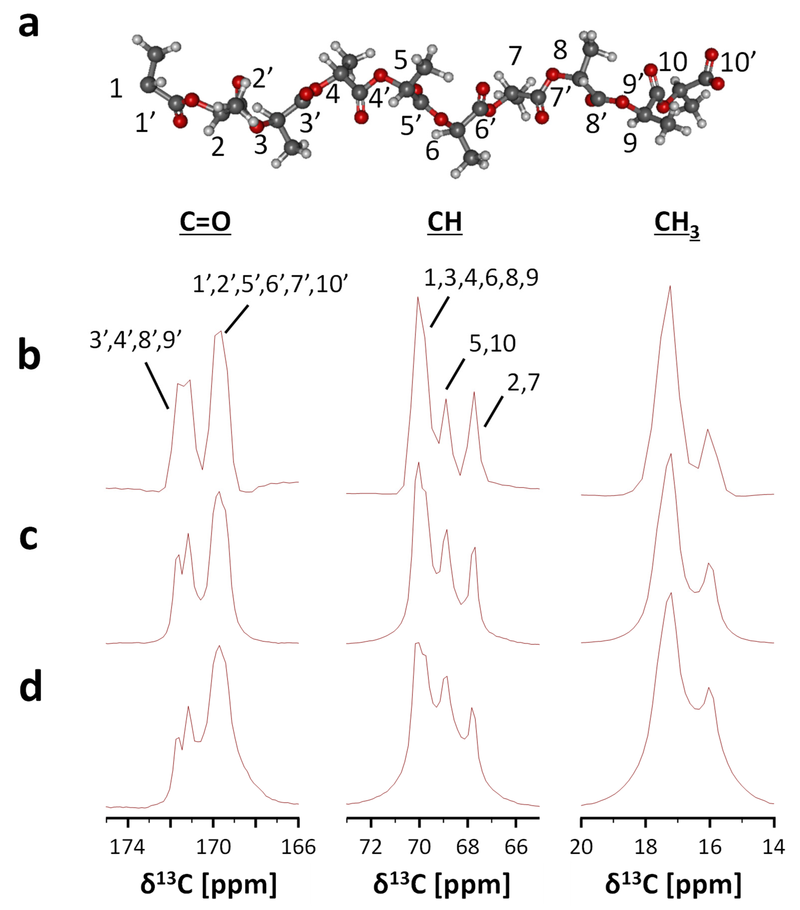
3.1. Features of 13C-CP/MAS and 1H Wide-Line NMR Spectra of PLA

The 13C-CP/MAS spectra were stacked before and after the degradation experiment, and the signal shape became sharper as the time of exposure to the decomposition environment increased (Figure S1a). By comparing the 13C-CP/MAS spectra after the decomposition experiments with those of previous studies [25,26], it was possible to determine from which functional groups of PLA the sharpened signals originated. These results indicated that the crystal ratio of PLA was enlarged by the degradation experiment, which may be due to the preferential hydrolysis of the amorphous component and the relative increase in the crystalline component in the sample [14]. From this result, we decided to use the NMR spectrum as an explanatory variable. The 1H wide-line NMR spectra were stacked before and after the degradation experiment (Figure S1b). However, no significant change in signal shape was observed after the decomposition experiment in comparison with that before the decomposition experiment. Therefore, it was considered that by using PCA, it is possible to capture minute changes in the signal shape and extract the characteristics of signals related to decomposition. First, Figure S2 shows the results of PCA for the 13C-CP/MAS spectra. In the PCA score plot, the difference in crystallinity could be determined by characterizing the difference in sample species. In the PCA loading plot, PC1 extracted a broad signal and PC2 extracted a sharp signal. In the 13C-CP/MAS spectra of the polymer, the amorphous-derived signal became broad and the crystal-derived signal became sharp [14,15]; thus, the characteristics of PC1 were classified as amorphous and PC2 was classified as crystalline. Figure S3 shows the results of PCA of the 1H wide-line NMR spectra. In the PCA score plot, the difference in crystallinity could be determined based on the characterization of the difference in sample species. In addition, in the PCA loading plot, PC1 extracted a broad signal and PC2 extracted a sharp signal. In the 1H wide-line NMR spectra of the polymer, the amorphous-derived signal was sharp, and the crystal-derived signal was broad [9,27]; thus, PC1 was classified as crystalline and PC2 was classified as amorphous. The total contribution of PC1 and PC2 was 99.5% for the PCA of 13C-CP/MAS spectra and 99.9% for the PCA of 1H wide-line NMR spectra. From this, it was possible to obtain most of the information on the NMR spectra by using only PC1 and PC2. If there are many explanatory variables, the calculation cost becomes enormous when performing machine learning. Therefore, it is possible to construct predictive models that maximize information while suppressing the calculation cost when utilizing a compression technique such as PCA.

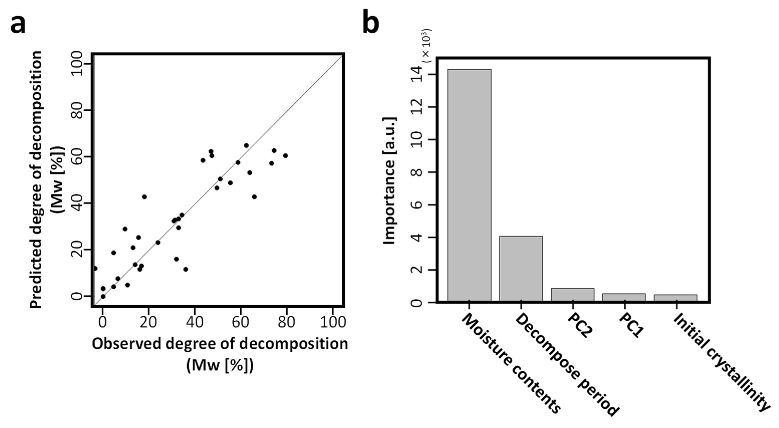
3.2. Validation of Decomposition Degree Predictive Models and Comparison of Contributing Factors

Firstly, a dataset for machine learning was created using the weight-loss ratio as an objective variable and the moisture content of the compost environment, degradation period, initial crystallinity, and features of 13C-CP/MAS spectra as explanatory variables. The decomposition degree predictive model was constructed using RF and XGBoost machine learning algorithms to process these data. The results of the prediction of data validation are shown in Figure S4. R2 was 0.38 for RF and 0.08 for XGBoost. RMSE was 0.76% for RF and 1.30% for XGBoost. Thus, RF had a higher prediction accuracy than XGBoost. However, we considered that the degree of decomposition cannot be predicted accurately, because the bivariate plots of observed and predicted weight-loss ratios did not follow a diagonal line and the variation was substantial. Therefore, we constructed a decomposition degree predictive model in which the objective variable was changed to Mw. The results of the prediction of validation data and a comparison of the factors of importance are shown in Figure 2.
R2 and RMSE were 0.78 and 10.78%, respectively. From these results, we found that a more accurate decomposition degree predictive model could be constructed by using Mw rather than weight-loss ratio as the objective variable. Next, we discussed the contributing factors for prediction. The moisture content in the compost environment and decomposition period had a significant effect on the degree of decomposition. The reason why the moisture content in the compost environment greatly affected the degradation degree was considered to be due to the primary degradation of PLA occurring by hydrolysis, and it was confirmed that the amount of moisture in the surrounding environment was extremely important during the early stage of degradation. In addition, the PC1 and PC2 obtained by PCA of the NMR spectra provided information on the crystalline and amorphous structure, which slightly affected the degree of decomposition. We also examined the construction of a decomposition degree predictive model using 1H wide-line spectra. The results of the prediction of validation data and comparison of factors of importance are shown in Figure S5. R2 and RMSE were 0.73 and 12.42%, respectively. Based on these results, the predictive model constructed using the 1H wide-line NMR spectra yielded lower predictive accuracy than using 13C-CP/MAS spectra, which was likely due to the good separability of the carbon chain signal, and the fact that the crystal structure information could be obtained more clearly with 13C-CP/MAS. Based on the importance of the predictive model, the moisture content in the compost environment and decomposition period had a significant effect on the degree of decomposition, while the factor of the crystalline or amorphous structure had little effect on the degree of decomposition. Furthermore, these results were similar to those which were obtained using 13C-CP/MAS.
Finally, the optimum decomposition degree, various analytical values, and experimental conditions were explored from virtual experiments that combined the constructed decomposition degree predictive model with Bayesian optimization. The NMR spectra were predicted by calculating the inner product of the PCA loadings and PC1 and PC2 scores at the optimal decomposition degree proposed by Bayesian optimization, and then calculating the restoration matrix. The stack diagram of the obtained predicted spectra and actual measured spectra is shown in Figure 3. Based on the comparison of the spectra, the spectra were predicted to have a higher crystal ratio. Predictions of the experimental conditions, such as moisture content in the compost environment, were also possible, but the predicted values of the degree of decomposition did not exceed the actual measured values. This was thought to be due to the influence of the range on the objective variables of machine learning. However, the results may be improved by implementing other machine learning methods to perform the verification calculations [28,29,30], which should be tested in future studies.

4. Conclusions

Degradation experiments were conducted to obtain the indices for the external environment, such as moisture content in a compost environment. The data were obtained from the experiments used to develop a model for predicting the degree of degradation, which was constructed by machine learning. The predictive model accurately predicted the degree of degradation by using the rate of decrease in Mw as the objective variable. The rank of importance of the influencing factors on the degree of degradation, from highest to lowest, was the moisture content in the compost environment, degradation period, information on crystalline and amorphous structure, and initial crystallinity. Furthermore, by combining the constructed predictive model with Bayesian optimization, it was possible to predict the experimental conditions and NMR spectra when the decomposition degree was optimized. Although the optimized decomposition degree did not exceed the measured value, the result may be improved by implementing other machine learning methods. In addition, by adding experimental conditions such as temperature and pH to this predictive model, it may be possible to construct a more accurate predictive model that can explore the decomposition factors in more detail. In addition, for virtual experiments on bio-based plastics other than PLA, the decomposition degree predictive model and Bayesian optimization used in this study might achieve optimal accuracy. As a result, it may be possible to reduce the experimental cost and obtain the experimental conditions and analytical values at an optimum decomposition degree while analyzing the decomposition factors. Knowledge obtained from such virtual experiments is expected to lead to the design and development of bio-based plastics.

Supplementary Materials

The following are available online at https://www.mdpi.com/2076-3417/11/6/2820/s1, Figure S1: Stacked plot of 13C-CP/MAS and 1H wide-line spectra of PLA during the compost-degradation experiments; Figure S2: PCA using the 13C-CP/MAS spectra; Figure S3: PCA using the 1H wide-line NMR spectra; Figure S4: The results of predictive modeling using the weight-loss ratio as the objective variable by RF and XGBoost; Figure S5: Predictive accuracy and importance of a predictive model of the degree of degradability using 1H wide-line NMR spectra; Table S1: List of PLA samples molded by the press-molding machine.

Author Contributions

R.Y., K.I. and J.K. designed the study; R.Y. and A.T. performed the experiments; R.Y. analyzed the data; R.Y. and K.I. programmed the analytical tools; all authors helped to prepare the manuscript and approved its submission. All authors have read and agreed to the published version of the manuscript.

Funding

This work was partially supported by a grant from the Agriculture, Forestry, and Fisheries Research Council, as well as the Strategic Innovation Program (SIP) from CAO (to J.K.).

Institutional Review Board Statement

Not applicable.

Informed Consent Statement

Not applicable.

Data Availability Statement

The data presented in this study are available on request from the corresponding author.

Acknowledgments

The authors thank D. Yokoyama, Y. Tsuboi, T. Matsumoto, H. Mikami, and S. Takayama for advice on the experiments.

Conflicts of Interest

The authors declare no conflict of interest.

References

  1. Borrelle, S.B.; Ringma, J.; Law, K.L.; Monnahan, C.C.; Lebreton, L.; McGivern, A.; Murphy, E.; Jambeck, J.; Leonard, G.H.; Hilleary, M.A.; et al. Predicted growth in plastic waste exceeds efforts to mitigate plastic pollution. Science 2020, 369, 1515–1518. [Google Scholar] [CrossRef]
  2. Kubowicz, S.; Booth, A.M. Biodegradability of Plastics: Challenges and misconceptions. Environ. Sci. Technol. 2017, 51, 12058–12060. [Google Scholar] [CrossRef]
  3. Mohanty, A.K.; Vivekanandhan, S.; Pin, J.-M.; Misra, M. Composites from renewable and sustainable resources: Challenges and innovations. Science 2018, 362, 536–542. [Google Scholar] [CrossRef] [PubMed] [Green Version]
  4. Ragauskas, A.J.; Williams, C.K.; Davison, B.H.; Britovsek, G.; Cairney, J.; Eckert, C.A.; Frederick, W.J., Jr.; Hallett, J.P.; Leak, D.J.; Liotta, C.L.; et al. The path forward for biofuels and biomaterials. Science 2006, 311, 484–489. [Google Scholar] [CrossRef] [PubMed] [Green Version]
  5. Drumright, R.E.; Gruber, P.R.; Henton, D.E. Polylactic Acid Technology. Adv. Mater. 2000, 12, 1841–1846. [Google Scholar] [CrossRef]
  6. Suganuma, K.; Horiuchi, K.; Matsuda, H.; Cheng, H.N.; Aoki, A.; Asakura, T. NMR analysis and chemical shift calculations of poly(lactic acid) dimer model compounds with different tacticities. Polym. J. 2012, 44, 838–844. [Google Scholar] [CrossRef] [Green Version]
  7. Paluch, P.; Pawlak, T.; Jeziorna, A.; Trebosc, J.; Hou, G.; Vega, A.J.; Amoureux, J.P.; Dracinsky, M.; Polenova, T.; Potrzebowski, M.J. Correction: Analysis of local molecular motions of aromatic sidechains in proteins by 2D and 3D fast MAS NMR spectroscopy and quantum mechanical calculations. Phys. Chem. Chem. Phys. 2017, 19, 21210–21210. [Google Scholar] [CrossRef] [PubMed] [Green Version]
  8. Takeda, K.; Kobayashi, Y.; Noda, Y.; Takegoshi, K. Inner-product NMR spectroscopy: A variant of covariance NMR spectroscopy. J. Magn. Reson. 2018, 297, 146–151. [Google Scholar] [CrossRef] [PubMed]
  9. Yamada, S.; Chikayama, E.; Kikuchi, J. Signal deconvolution and generative topographic mapping regression for solid-state NMR of multi-component materials. Int. J. Mol. Sci. 2021, 22, 1086. [Google Scholar] [CrossRef]
  10. Sakurai, A.; Yada, K.; Simomura, T.; Ju, S.; Kashiwagi, M.; Okada, H.; Nagao, T.; Tsuda, K.; Shiomi, J. Ultranarrow-band wavelength-selective thermal emission with aperiodic multilayered metamaterials designed by Bayesian optimization. ACS Cent. Sci. 2019, 5, 319–326. [Google Scholar] [CrossRef]
  11. Numata, K.; Asano, A.; Nakazawa, Y. Solid-state and time domain NMR to elucidate degradation behavior of thermally aged poly (urea-urethane). Polym. Degrad. Stab. 2020, 172, 109052. [Google Scholar] [CrossRef]
  12. Mori, T.; Chikayama, E.; Tsuboi, Y.; Ishida, N.; Shisa, N.; Noritake, Y.; Moriya, S.; Kikuchi, J. Exploring the conformational space of amorphous cellulose using NMR chemical shifts. Carbohydr. Polym. 2012, 90, 1197–1203. [Google Scholar] [CrossRef] [Green Version]
  13. Okushita, K.; Chikayama, E.; Kikuchi, J. Solubilization mechanism and characterization of the structural change of bacterial cellulose in regenerated states through ionic liquid treatment. Biomacromolecules 2012, 13, 1323–1330. [Google Scholar] [CrossRef] [PubMed]
  14. Thakur, K.A.M.; Kean, R.T.; Zupfer, J.M.; Buehler, N.U.; Doscotch, M.A.; Munson, E.J. Solid state 13C CP-MAS NMR studies of the crystallinity and morphology of poly(l-lactide). Macromolecules 1996, 29, 8844–8851. [Google Scholar] [CrossRef]
  15. Tsuji, H.; Kamo, S.; Horii, F. Solid-state 13C NMR analyses of the structures of crystallized and quenched poly(lactide)s: Effects of crystallinity, water absorption, hydrolytic degradation, and tacticity. Polymer 2010, 51, 2215–2220. [Google Scholar] [CrossRef]
  16. Gopakumar, A.M.; Balachandran, P.V.; Xue, D.; Gubernatis, J.E.; Lookman, T. Multi-objective optimization for materials discovery via adaptive design. Sci. Rep. 2018, 8, 1–12. [Google Scholar] [CrossRef] [PubMed] [Green Version]
  17. Ju, S.; Shiga, T.; Feng, L.; Hou, Z.; Tsuda, K.; Shiomi, J. Designing nanostructures for phonon transport via Bayesian optimization. Phys. Rev. X 2017, 7, 021024. [Google Scholar] [CrossRef] [Green Version]
  18. Seko, A.; Togo, A.; Hayashi, H.; Tsuda, K.; Chaput, L.; Tanaka, I. Prediction of low-thermal-conductivity compounds with first-principles anharmonic lattice-dynamics calculations and Bayesian optimization. Phys. Rev. Lett. 2015, 115, 205901. [Google Scholar] [CrossRef] [PubMed]
  19. Spaccini, R.; Todisco, D.; Drosos, M.; Nebbioso, A.; Piccolo, A. Decomposition of bio-degradable plastic polymer in a real on-farm composting process. Chem. Biol. Technol. Agric. 2016, 3, 1–12. [Google Scholar] [CrossRef] [Green Version]
  20. Yamazawa, A.; Iikura, T.; Shino, A.; Date, Y.; Kikuchi, J. Solid-, solution-, and gas-state NMR monitoring of 13C-cellulose degradation in an anaerobic microbial ecosystem. Molecules 2013, 18, 9021–9033. [Google Scholar] [CrossRef] [Green Version]
  21. Breiman, L. Random forests. Mach. Learn. 2001, 45, 5–32. [Google Scholar] [CrossRef] [Green Version]
  22. Chen, T.; Guestrin, C. Xgboost: A scalable tree boosting system. arXiv 2016, arXiv:1603.02754. [Google Scholar]
  23. Kuhn, M. Building predictive models in R using the caret package. J. Stat. Softw. 2008, 28, 1–26. [Google Scholar] [CrossRef] [Green Version]
  24. Snoek, J.; Larochelle, H.; Adams, R.P. Practical bayesian optimization of machine learning algorithms. Adv. Neural Inf. Process. Syst. 2012, 26, 2951–2959. [Google Scholar]
  25. Pawlak, T.; Jaworska, M.; Potrzebowski, M.J. NMR crystallography of α-poly(l-lactide). Phys. Chem. Chem. Phys. 2013, 15, 3137–3145. [Google Scholar] [CrossRef] [PubMed]
  26. Suganuma, K.; Asakura, T.; Oshimura, M.; Hirano, T.; Ute, K.; Cheng, H.N. NMR Analysis of poly(lactic acid) via statistical models. Polymers 2019, 11, 725. [Google Scholar] [CrossRef] [PubMed] [Green Version]
  27. Schäler, K.; Roos, M.; Micke, P.; Golitsyn, Y.; Seidlitz, A.; Thurn-Albrecht, T.; Schneider, H.; Hempel, G.; Saalwächter, K. Basic principles of static proton low-resolution spin diffusion NMR in nanophase-separated materials with mobility contrast. Solid State Nucl. Magn. Reson. 2015, 72, 50–63. [Google Scholar] [CrossRef]
  28. Ito, K.; Obuchi, Y.; Chikayama, E.; Date, Y.; Kikuchi, J. Exploratory machine-learned theoretical chemical shifts can closely predict metabolic mixture signals. Chem. Sci. 2018, 9, 8213–8220. [Google Scholar] [CrossRef] [Green Version]
  29. Gerrard, W.; Bratholm, L.A.; Packer, M.; Mulholland, A.J.; Glowacki, D.R.; Butts, C.P. IMPRESSION—Prediction of NMR parameters for 3-dimensional chemical structures using machine learning with near quantum chemical accuracy. Chem. Sci. 2020, 11, 508–515. [Google Scholar] [CrossRef] [Green Version]
  30. Das, S.; Edison, A.S.; Merz, K.M. Metabolite structure assignment using in silico NMR techniques. Anal. Chem. 2020, 92, 10412–10419. [Google Scholar] [CrossRef]
  31. Wasanasuk, K.; Tashiro, K.; Hanesaka, M.; Ohhara, T.; Kurihara, K.; Kuroki, R.; Tamada, T.; Ozeki, T.; Kanamoto, T. Crystal structure analysis of poly(l-lactic acid) α form on the basis of the 2-dimensional wide-angle synchrotron x-ray and neutron diffraction measurements. Macromolecules 2011, 44, 6441–6452. [Google Scholar] [CrossRef]
Figure 1. Concept of real and virtual degradable experiments in this study. Actual decomposition experiments were performed to obtain experimental conditions and various analytical data values (left). The optimum decomposition degree, various analytical values, and experimental conditions were explored by virtual experiments combining with a predictive model and Bayesian optimization method (right).
Applsci 11 02820 g001
Figure 2. The results of predictive modeling of the degree of decomposition using the weight average molecular weight (Mw), analytical values, experimental conditions, and principal component analysis (PCA) scores of cross-polarization and magic angle spinning (13C-CP/MAS spectra) using the random forest (RF) machine learning algorithm. (a) A bivariate plot of the observed and predicted Mw of validation data. R2 is 0.78 and RMSE is 10.78%. (b) Bar chart of importance in the decomposition degree predictive model. Details of PC1 and PC2 scores used for machine learning are shown in Figure S2.
Applsci 11 02820 g002
Figure 3. (a) 3D chemical structure of PLA from wide-angle neutron diffraction data [31], and the numbers on atoms were annotated with reference to Pawlak et al. (2013) [25]. (b) The predicted 13C-CP/MAS spectrum was constructed from the dot product calculation of the PCA loadings and predicted PCA scores obtained from the predictive model and Bayesian optimization. From left to right, the carbonyl group (C=O), methine group (CH), and methyl group (CH3) are shown. The experimental 13C-CP/MAS spectra of S/A samples (c) exposed to the degradation environment for 3 weeks and (d) before the degradation experiment.
Applsci 11 02820 g003
Publisher’s Note: MDPI stays neutral with regard to jurisdictional claims in published maps and institutional affiliations.

