
Automated Optical Inspection System for O-Ring Based on Photometric Stereo and Machine Vision


Abstract
:1. Introduction
2. The Proposed System
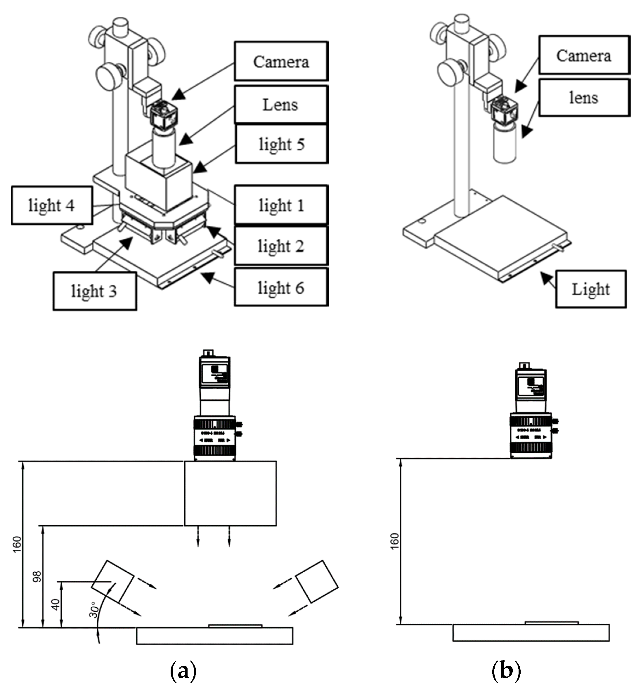
2.1. Hardware Architecture
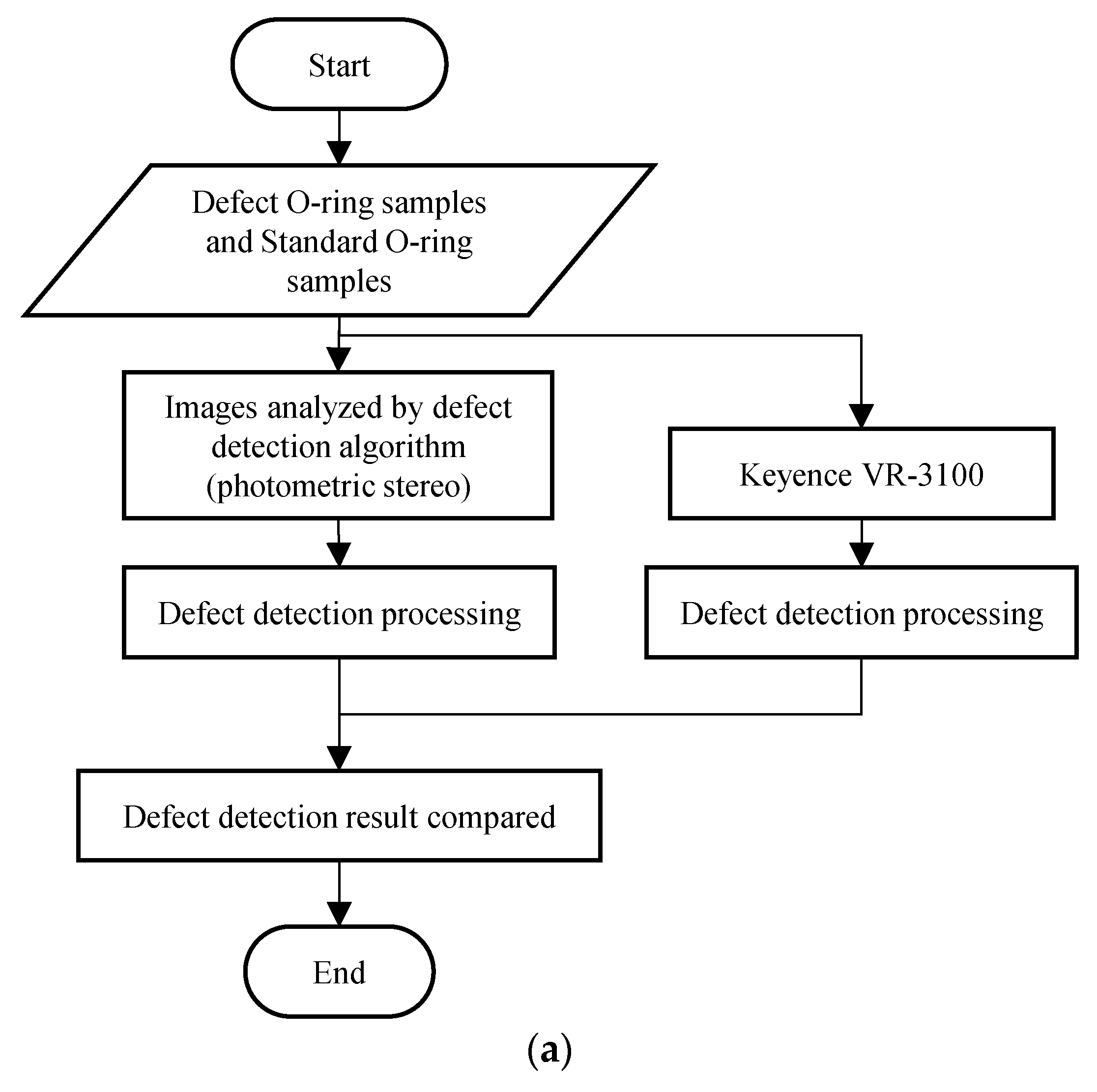
2.2. Processing of Defect Detection
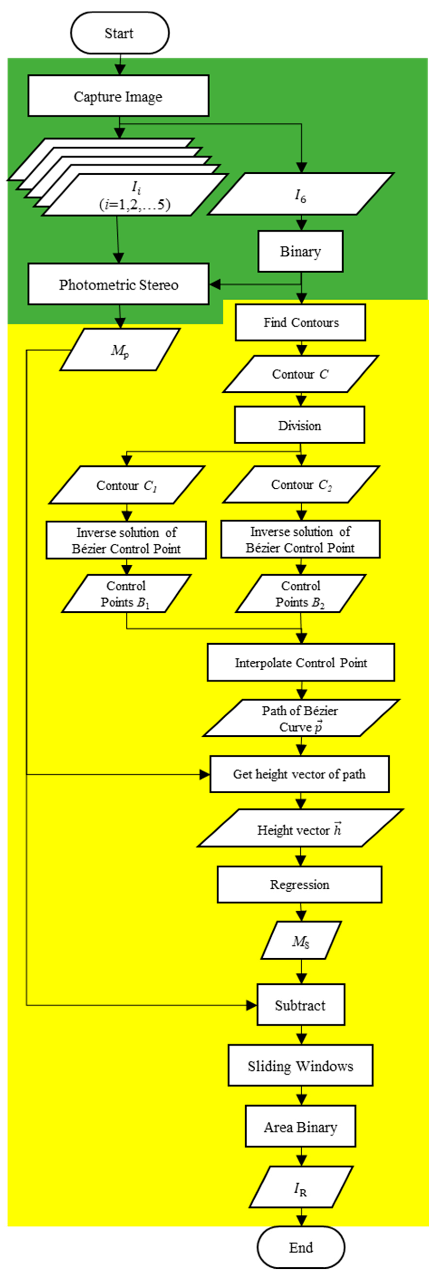
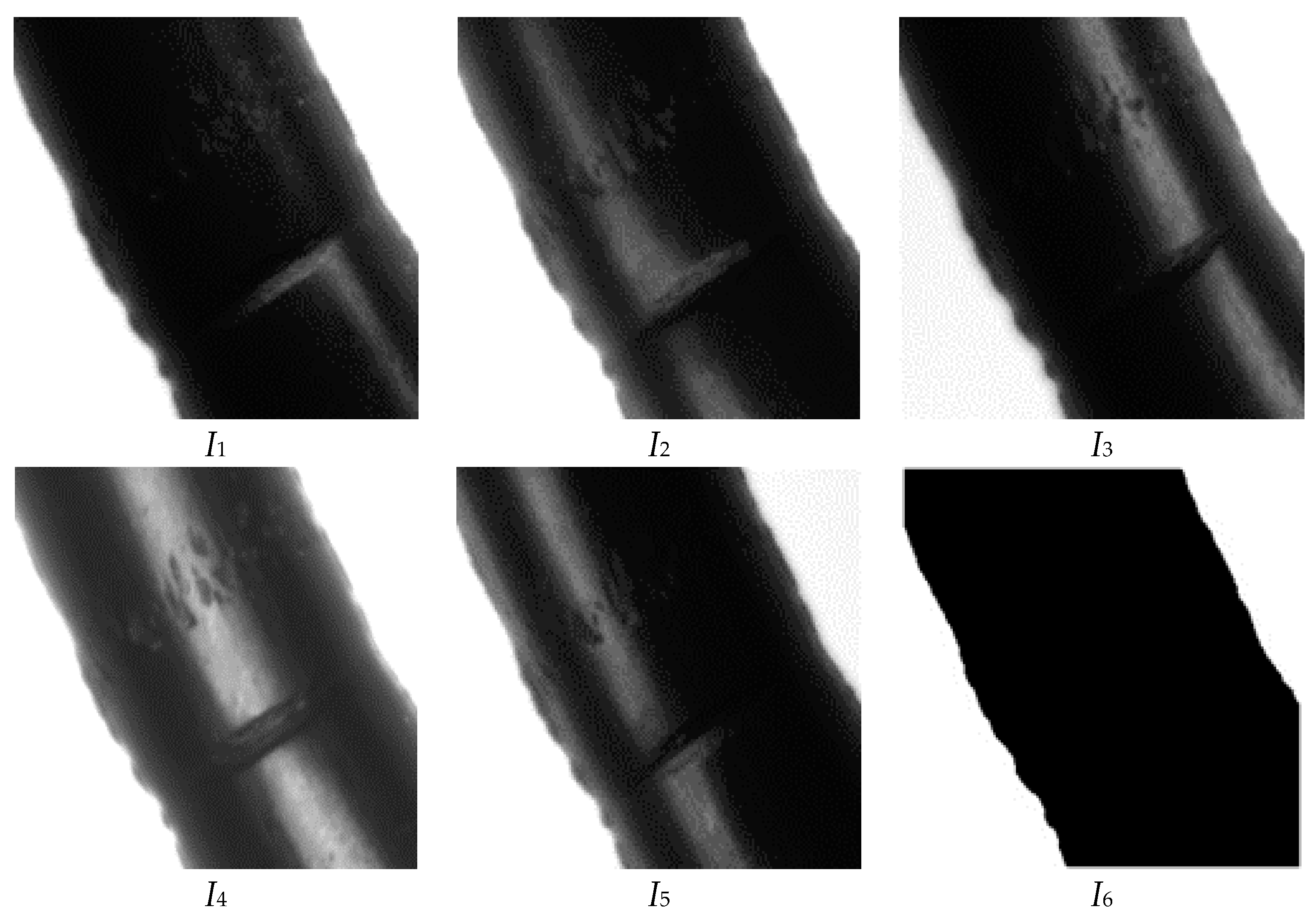
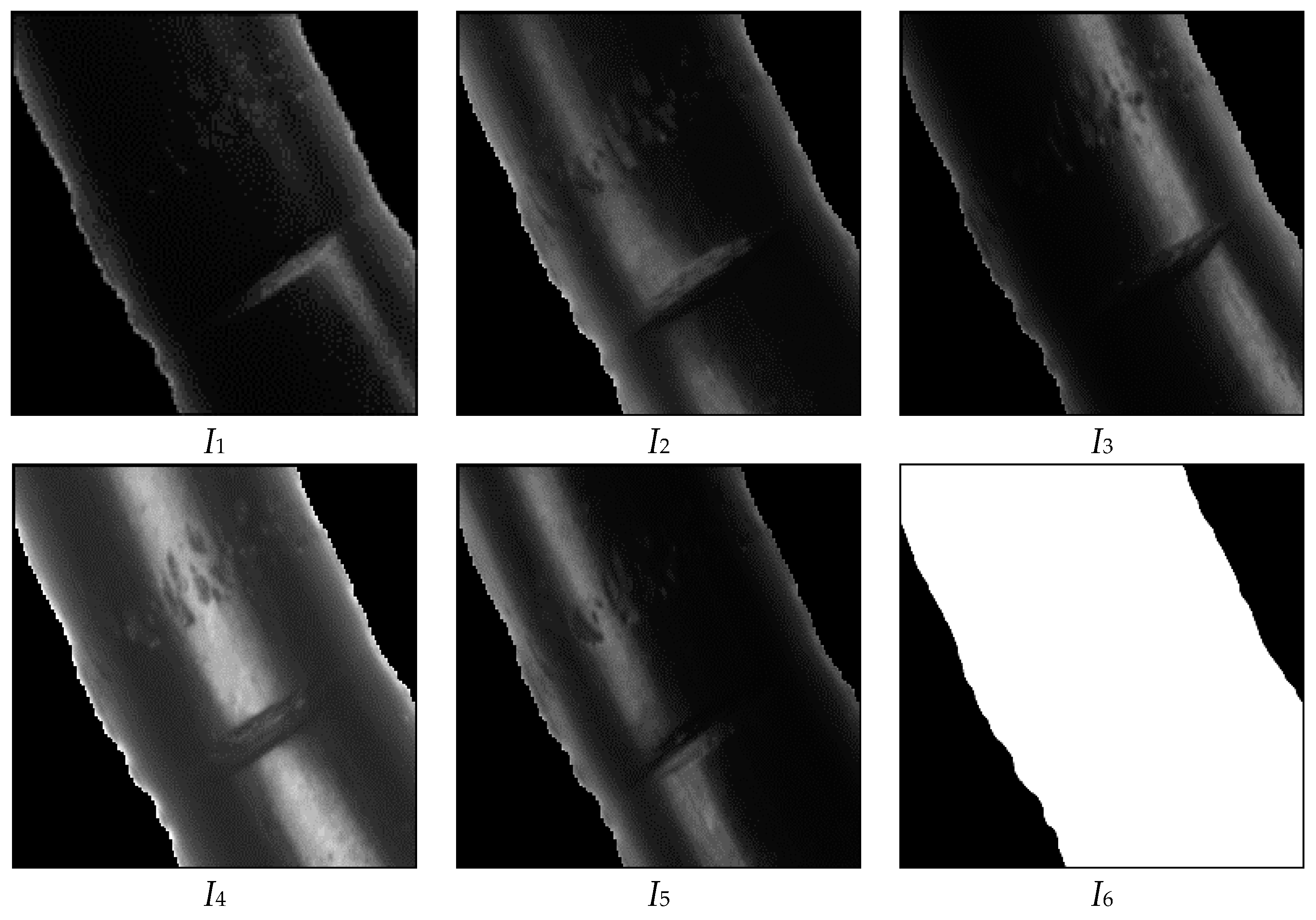
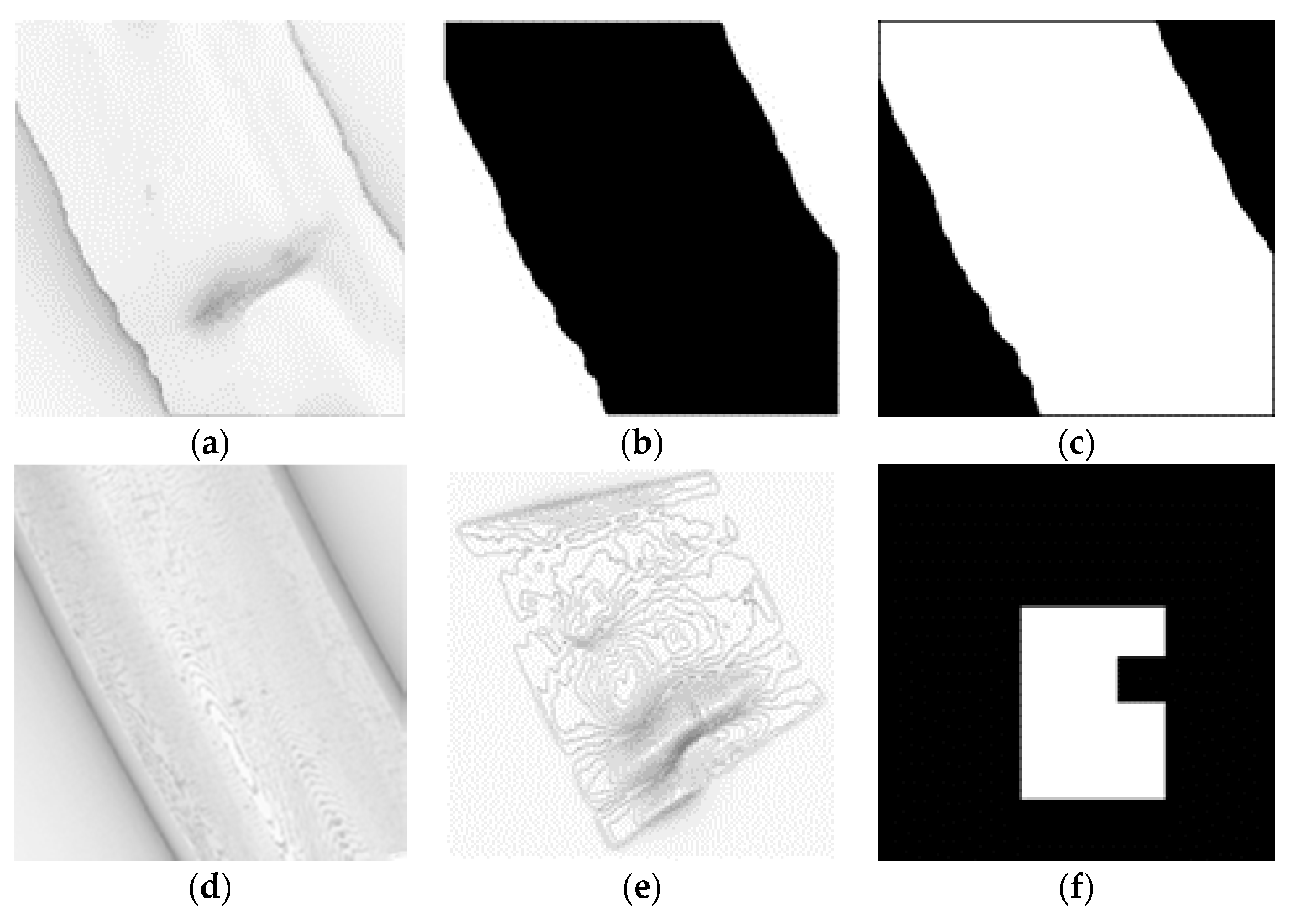
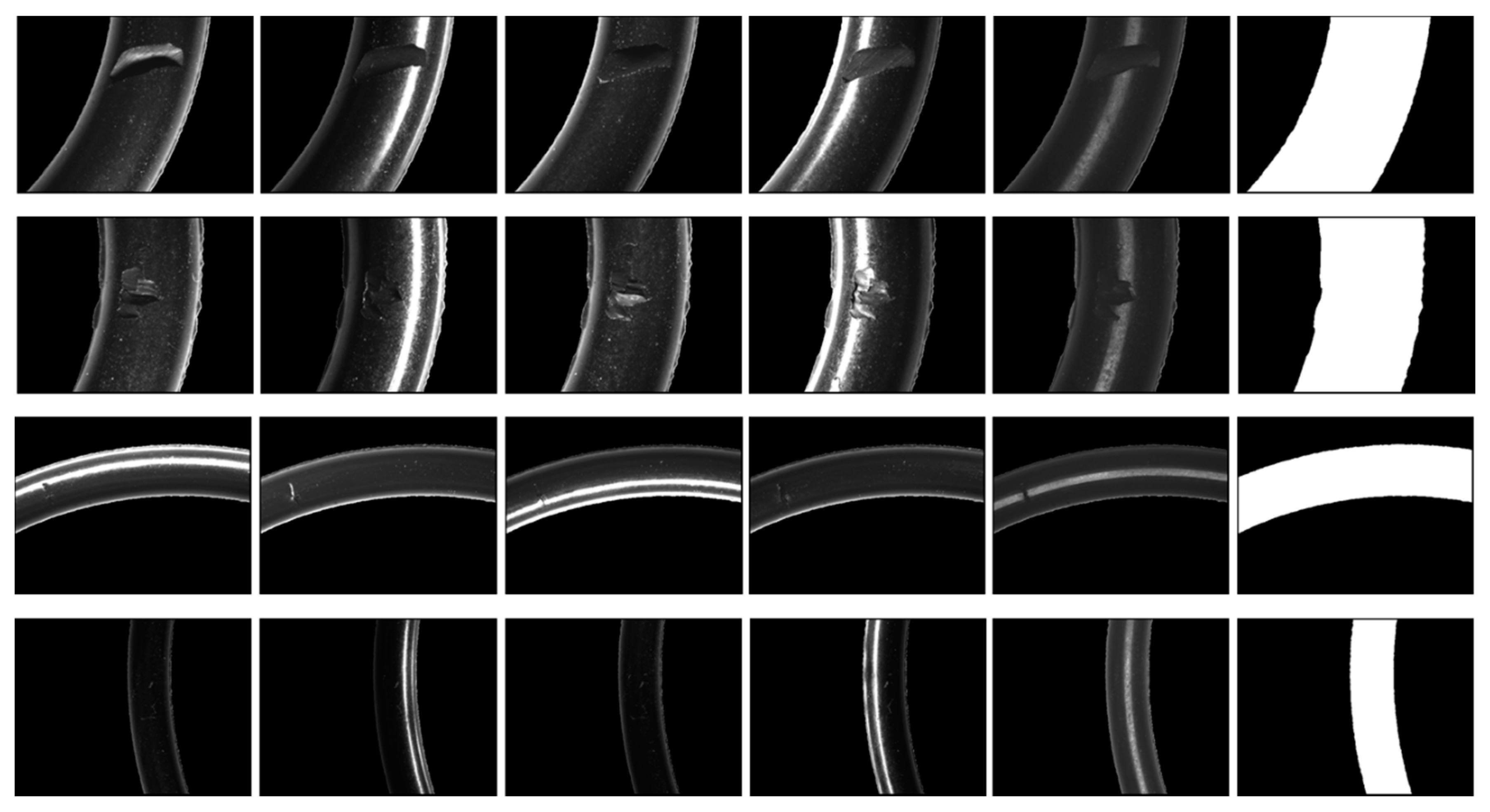
- Make a binary mask (Figure 7 I6) by using I6. Then, we used this mask to flit background information to reduce background noise effectively.
- Normalize image by using function (1). Which I(x, y) is a grayscale pixel value at position (x, y) of image.
- Define image moment as centroid and calculate maximum distance to mask edge r.
- Calculate light source direction vectors using the function (8).
- Define normal relative surface normal image N by using the function (10).
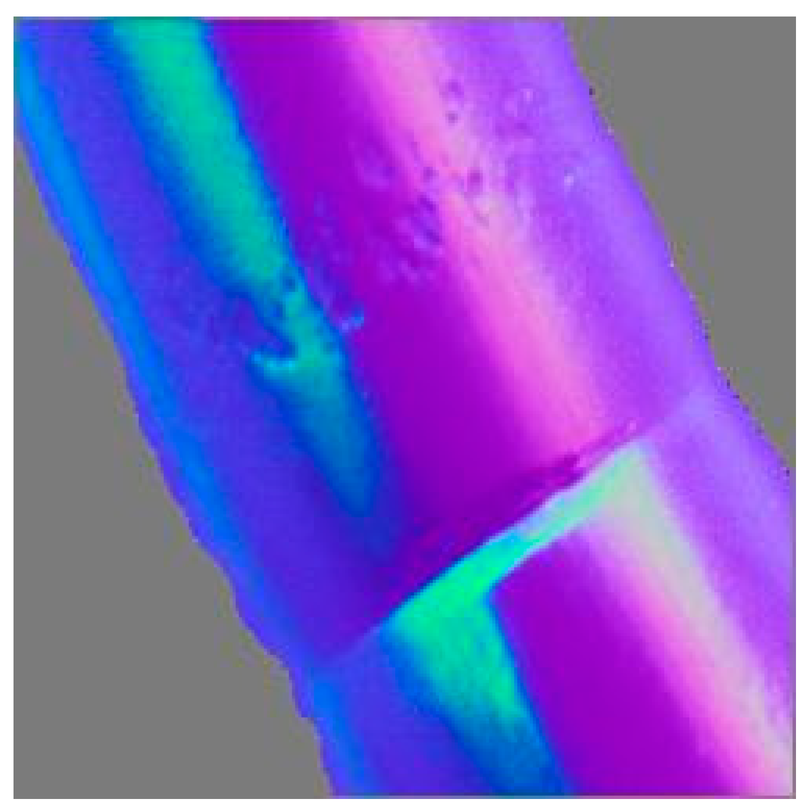
- Calculate unit vector field (Figure 8) by the function (11).
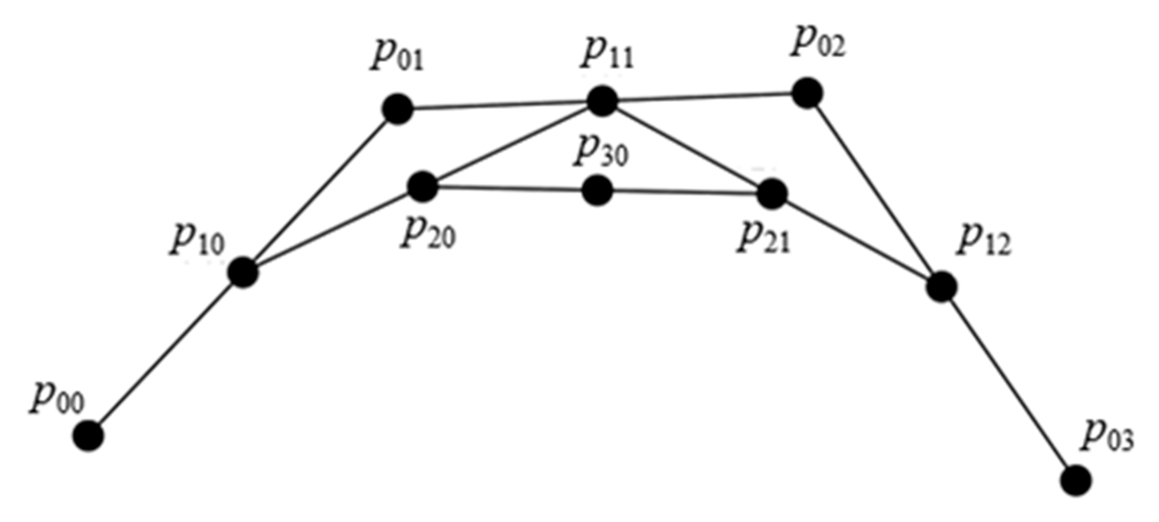
- First, we transfer unit vector field to triangle mesh. Then define each vertex point as Pi (i = 0, 1, 2) as function (12). Furthermore, each vertex point’s relative surface normal vector (i = 0, 1, 2). At last, we can define by using the function (13).
- Now, we can solve each vertex point’s relative surface normal vector (i = 0, 1, 2) by using the function (14) and unit vector field .
- The deep of the triangle mesh can be rewritten as an overdetermined set. So, in the image resolution would include the amount triangle. That is amount linear equation. Each triangle contains two linear equations as the function (16).
- We define A equal all of constant relative with z, and B equal and . Then, we can get the relative height of each pixel Z by using the function (14).
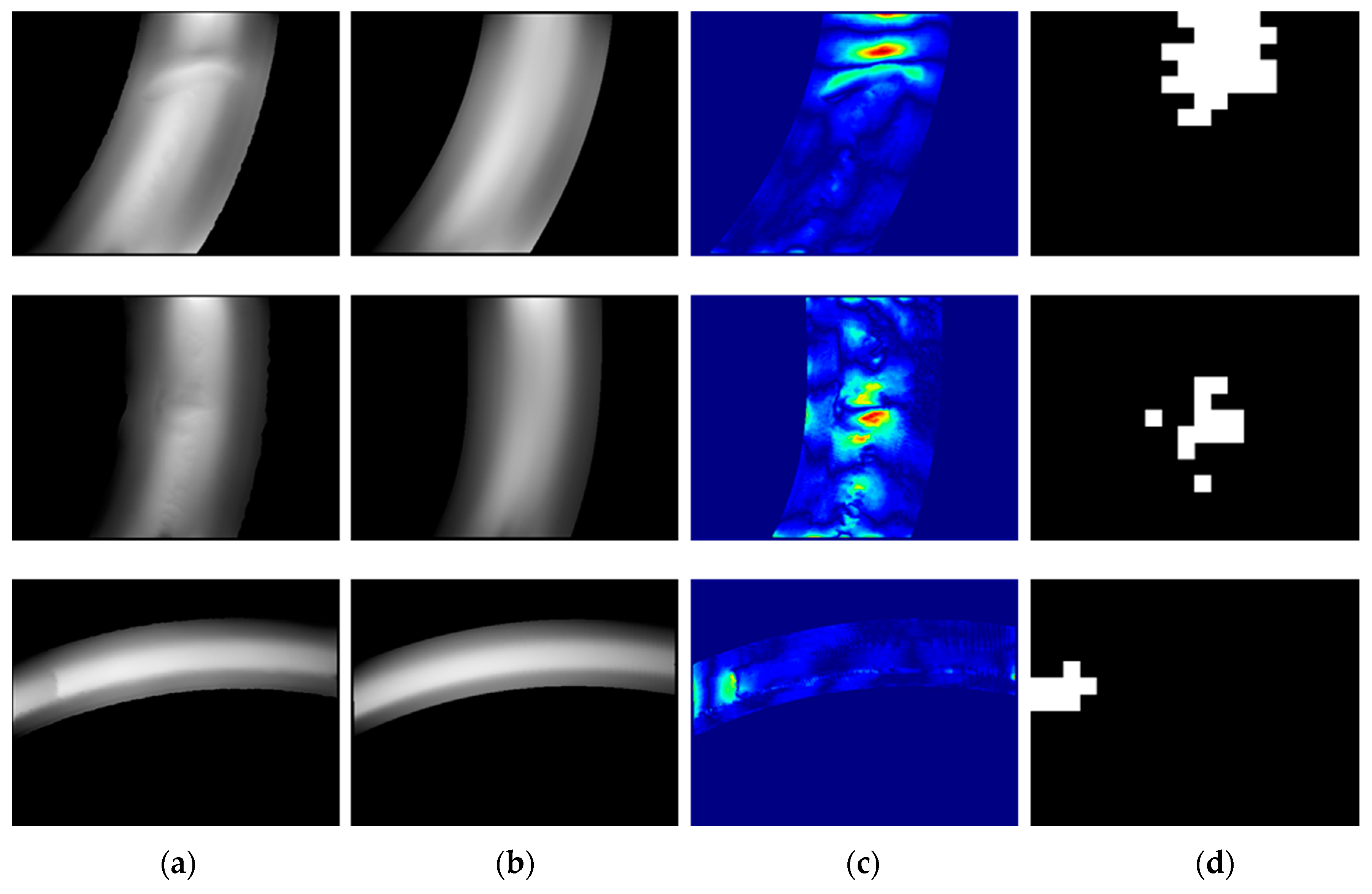
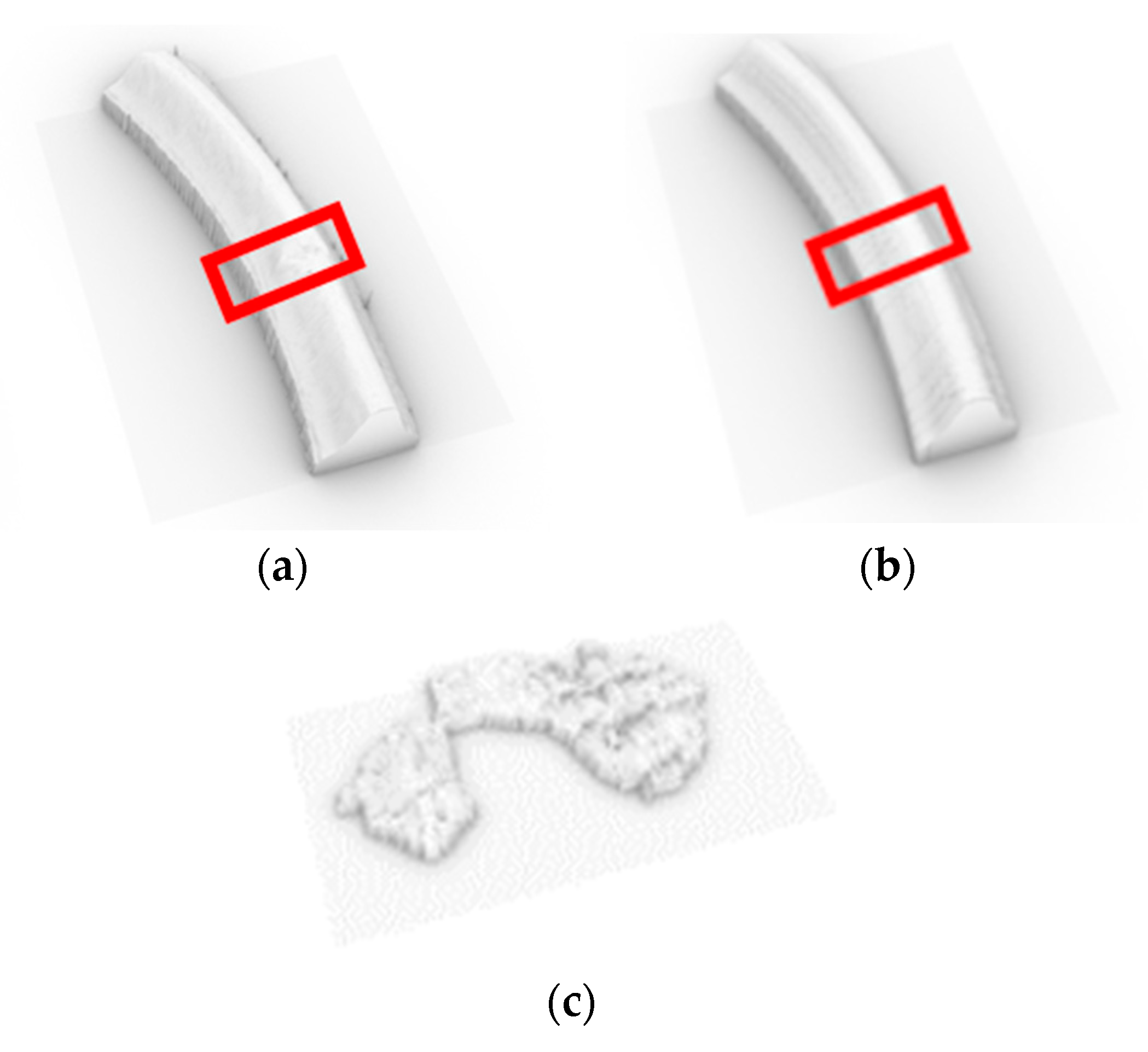
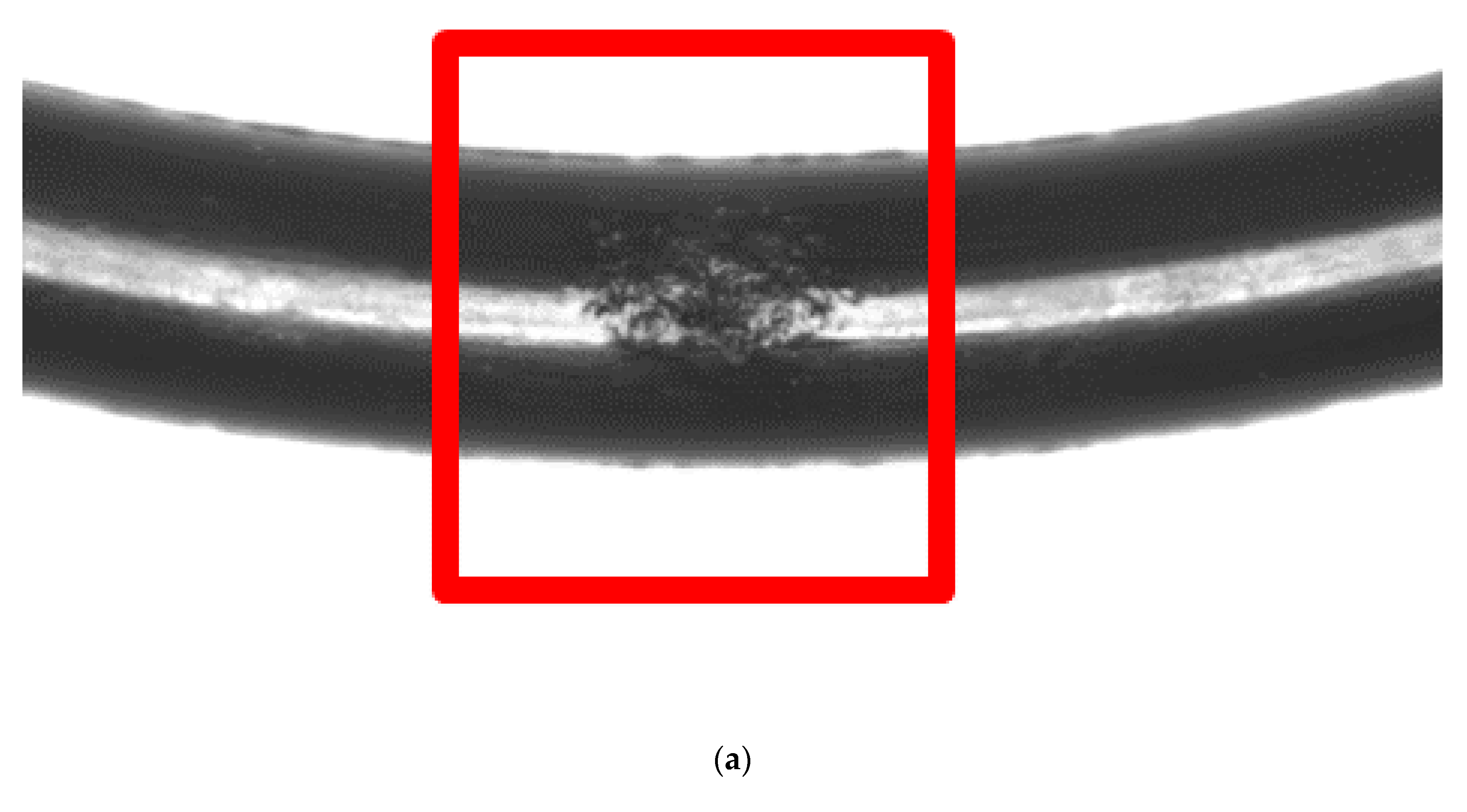
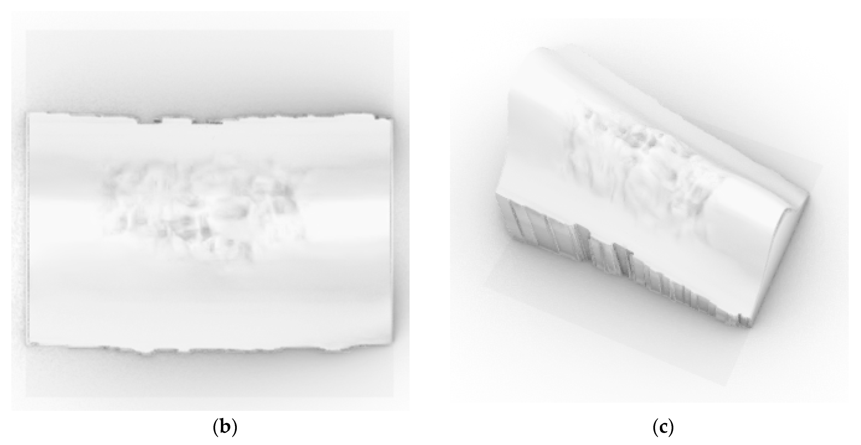
- At last, we create a 2.5-D model by using the photometric stereo method. The result is shown in Figure 9a. With the photometric stereo method, errors resulting from surface dirt in the inspection process were effectively prevented.
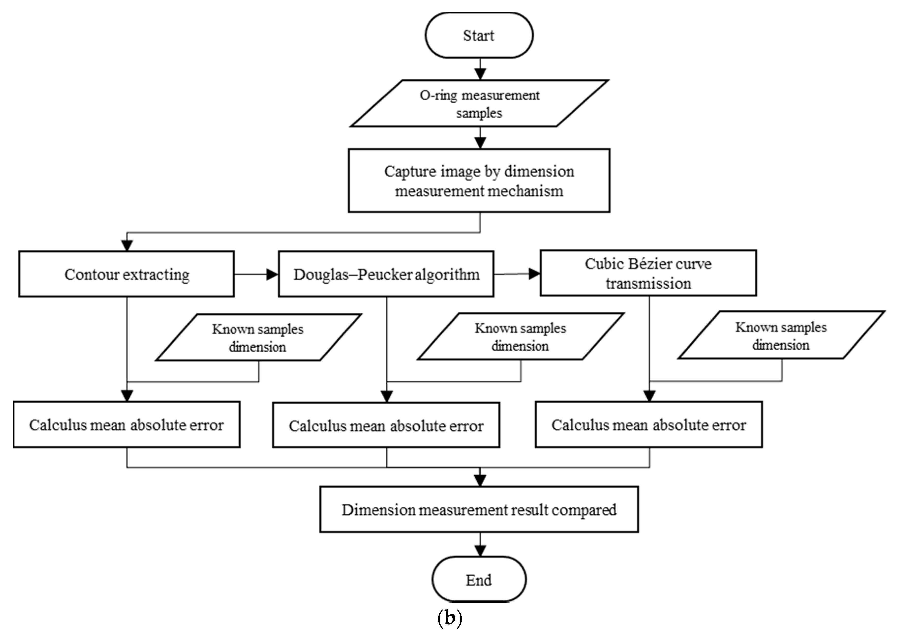
2.3. Processing of Dimension Measurement
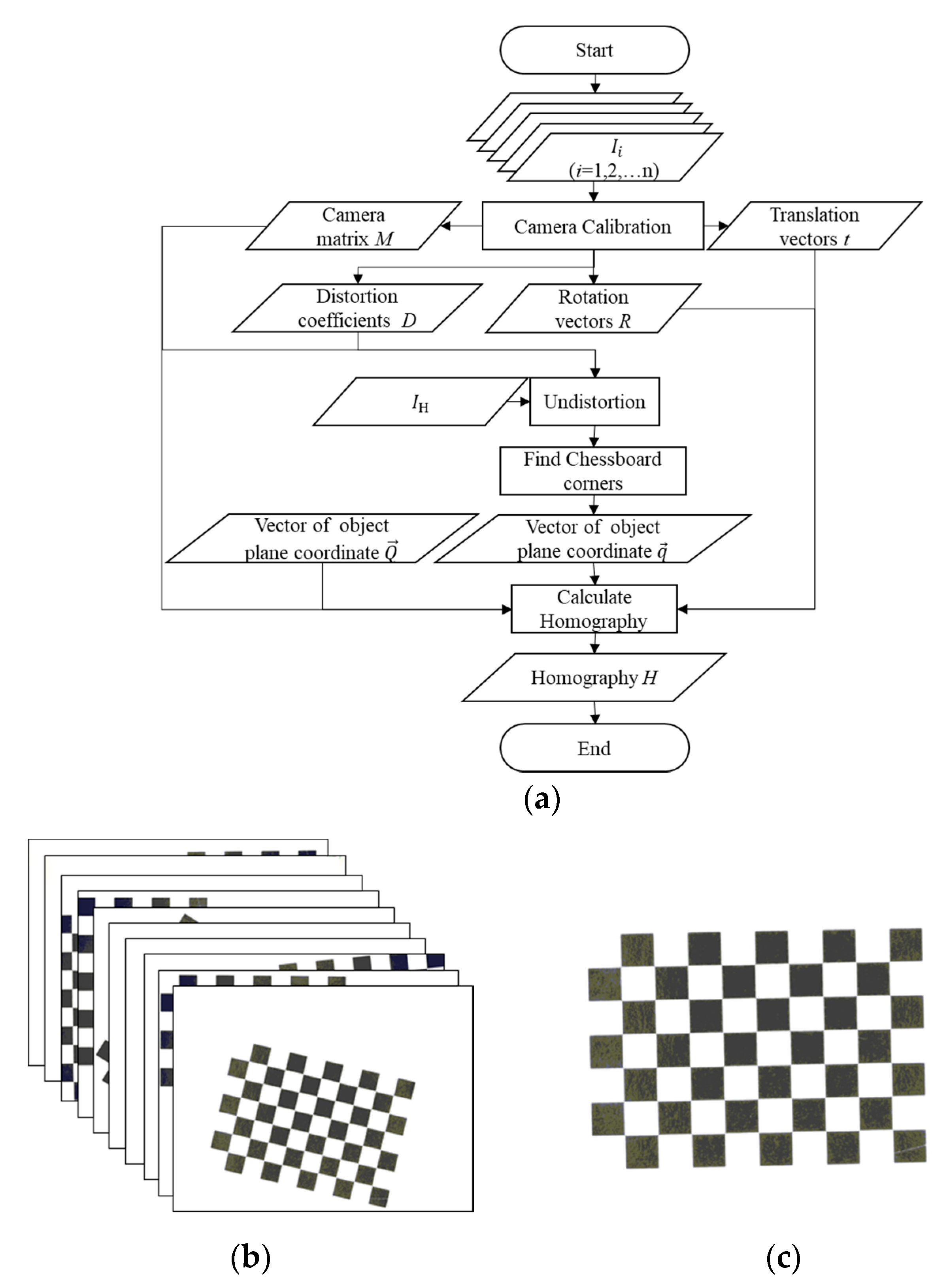
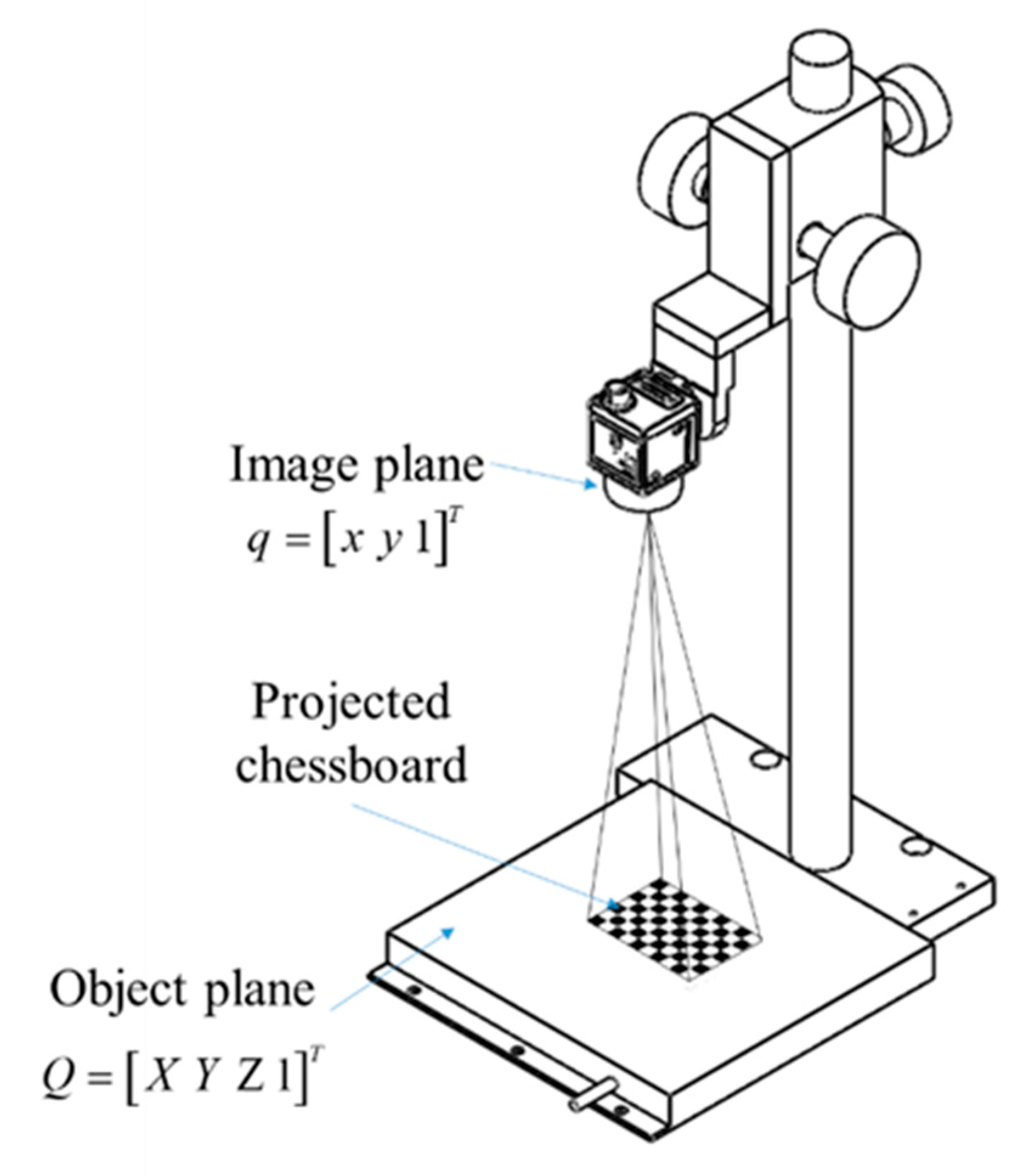
2.3.1. Pre-Processing of Dimension Measurement
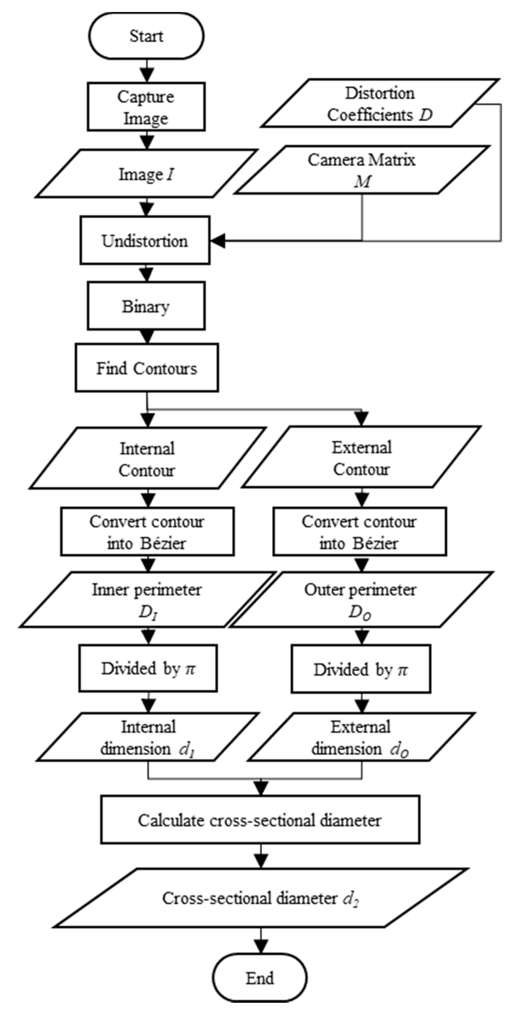
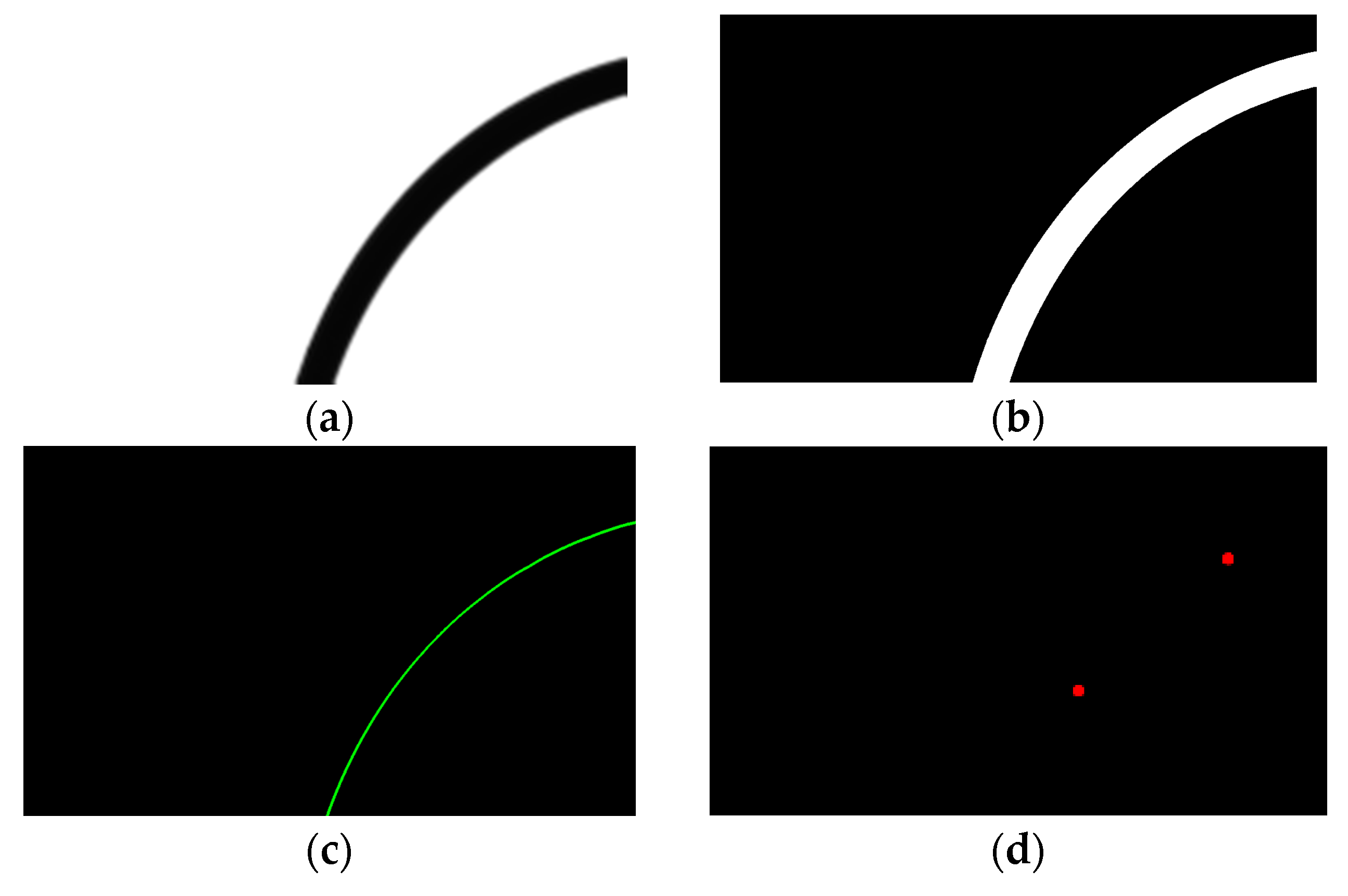
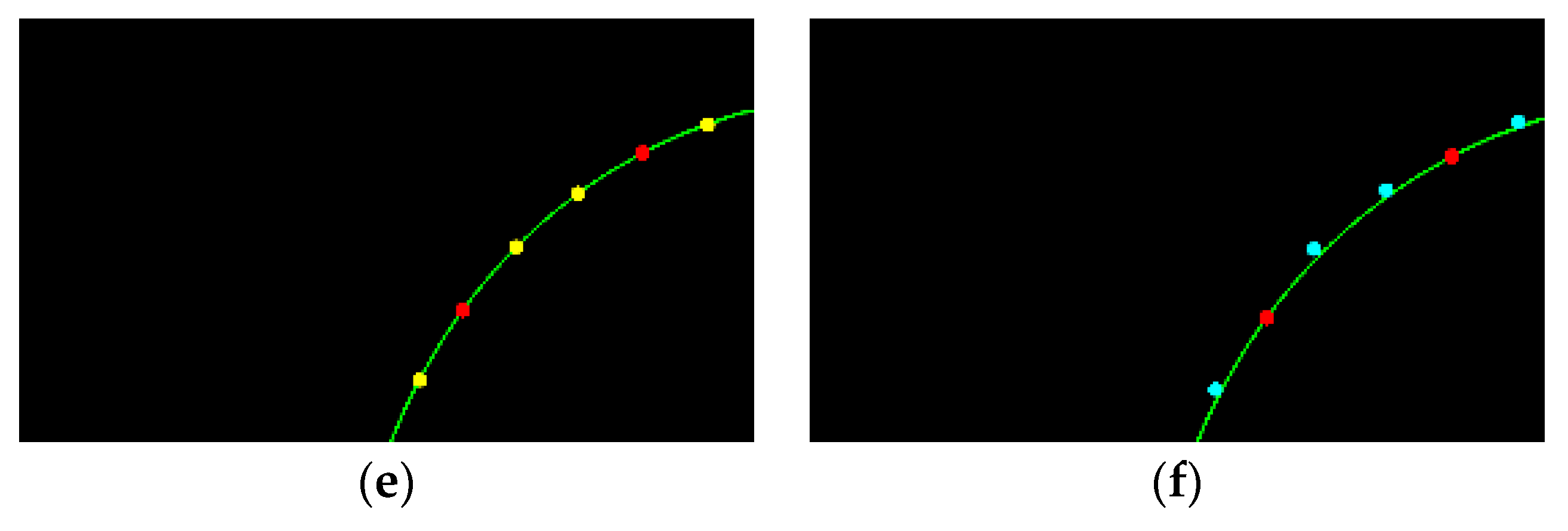
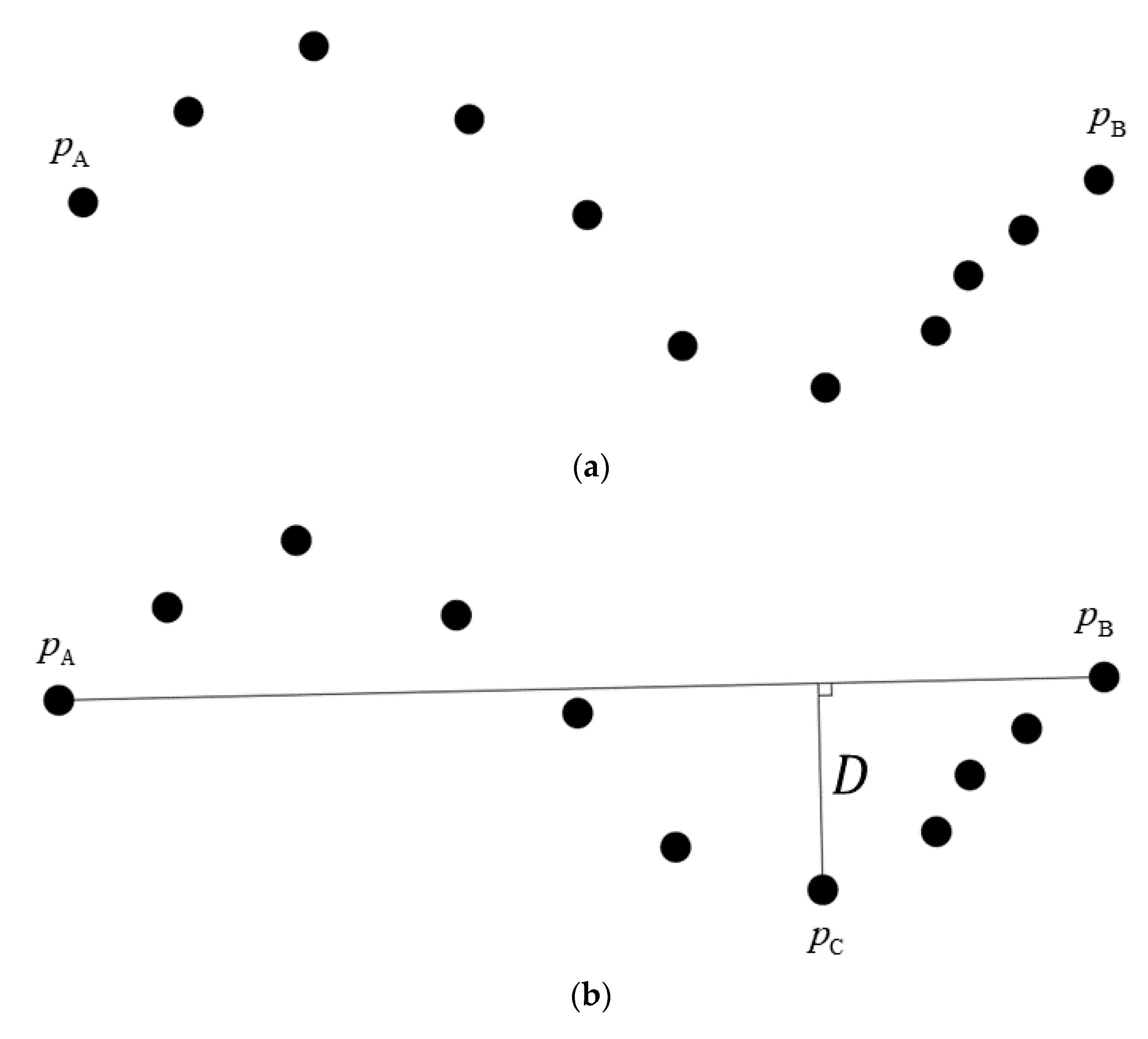
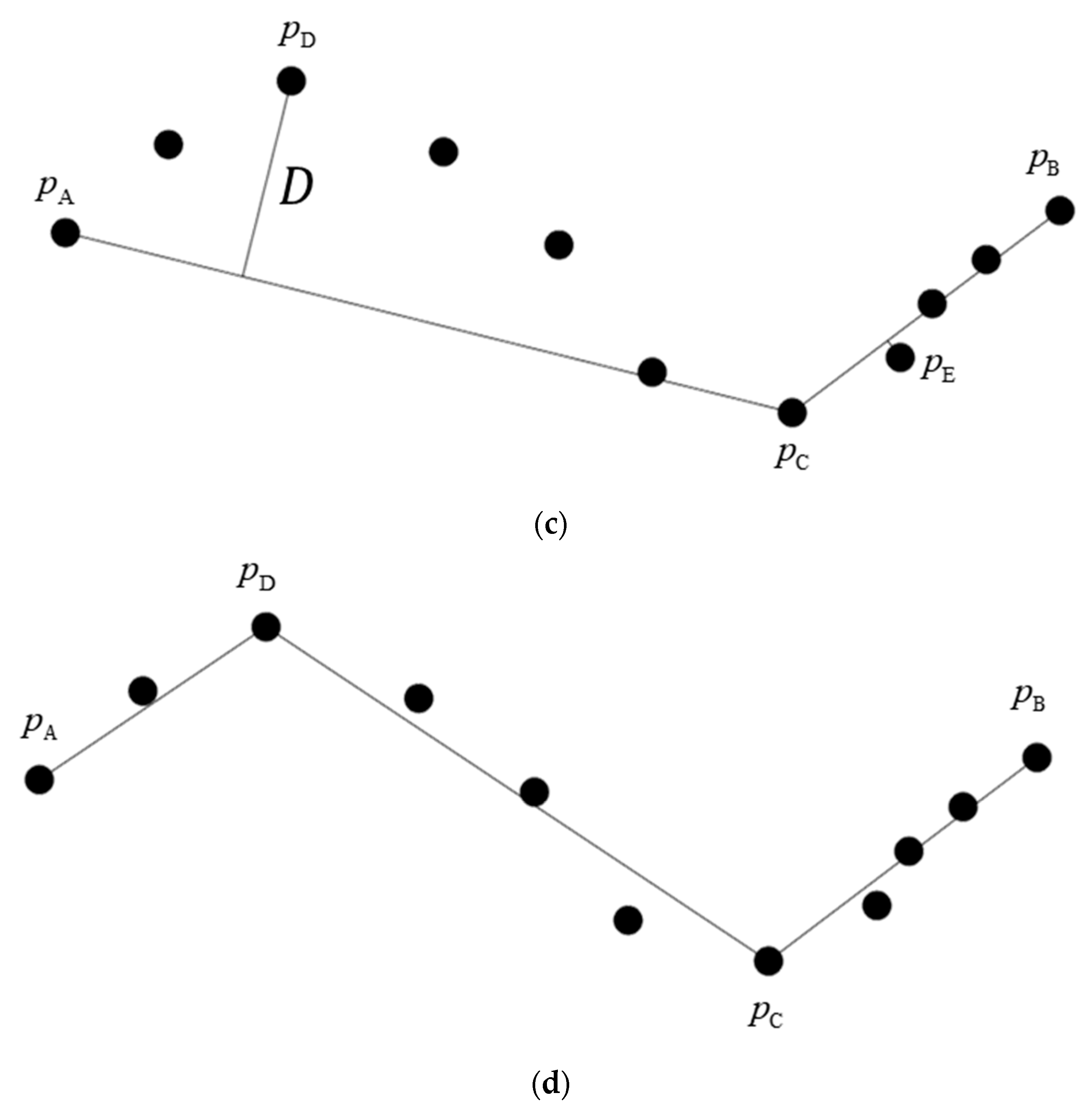
2.3.2. Dimension Measurement Processes
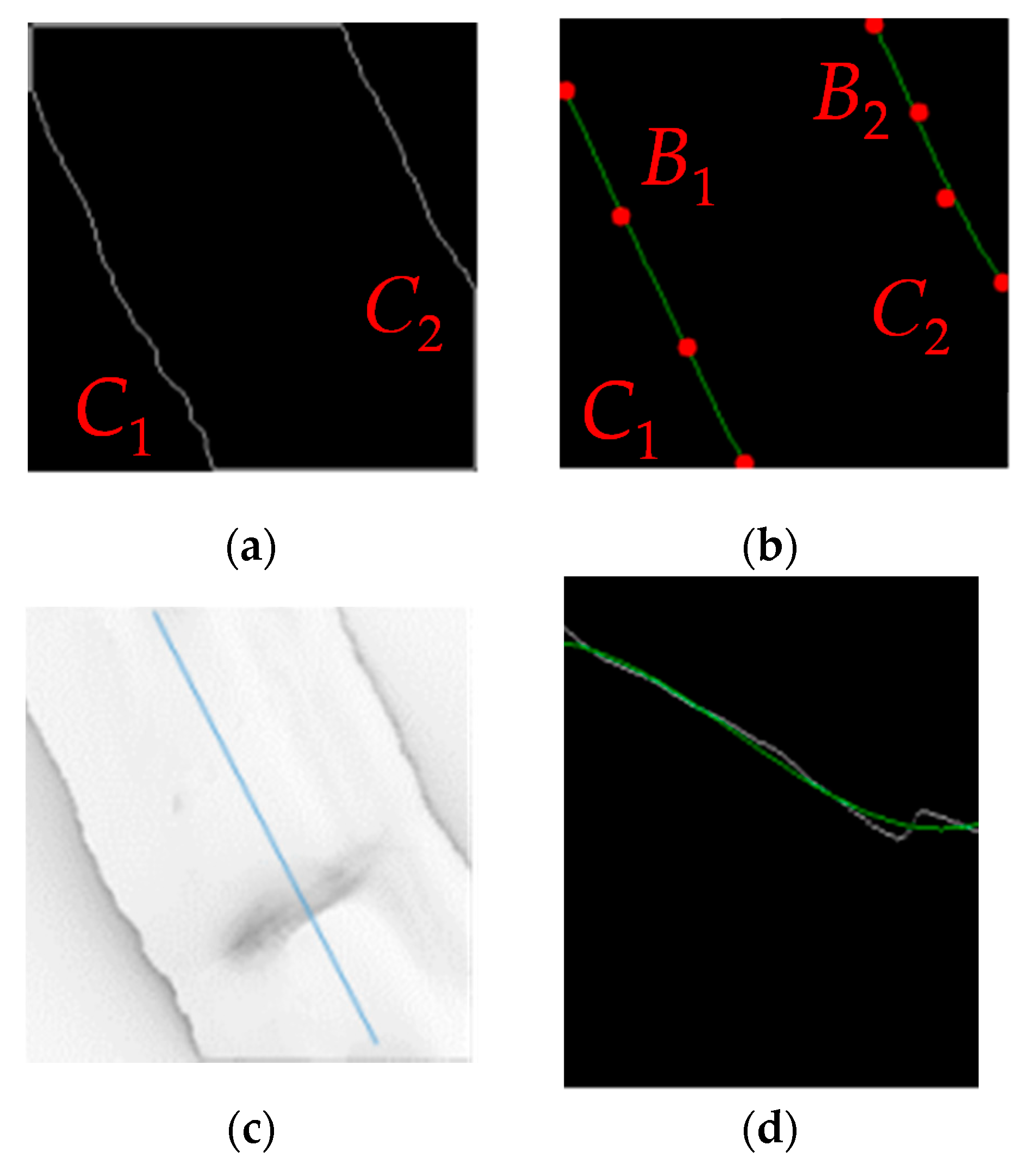
- Connect start point PA and end point PB. Then, find the furthest point PC and calculate the distance D from the point PC to the line (Figure 16b).
- If the distance D from the point PC to the line is bigger than the threshold we settled, divide the contour into two parts. Then, calculate the distance D from the point to the line, respectively (Figure 16c).
- Else if all of the distance D from the point to the line is smaller than the threshold finish the approximate operation.
3. O-Ring Database
3.1. Database for Defect Detection
3.1.1. DPS (Database of Photometric Stereo Model)
3.1.2. DK (Database of Raw Data with Profilometer)
3.2. Database for Dimension Measurement
3.2.1. DVT (Database of the Verified Samples Be Made of T6061)
3.2.2. DSI (Database of the Standard Sample Regulated by ISO
3.2.3. DSP (Database of the Standard Sample with External Pressure)
4. Experiment Results and Discussion
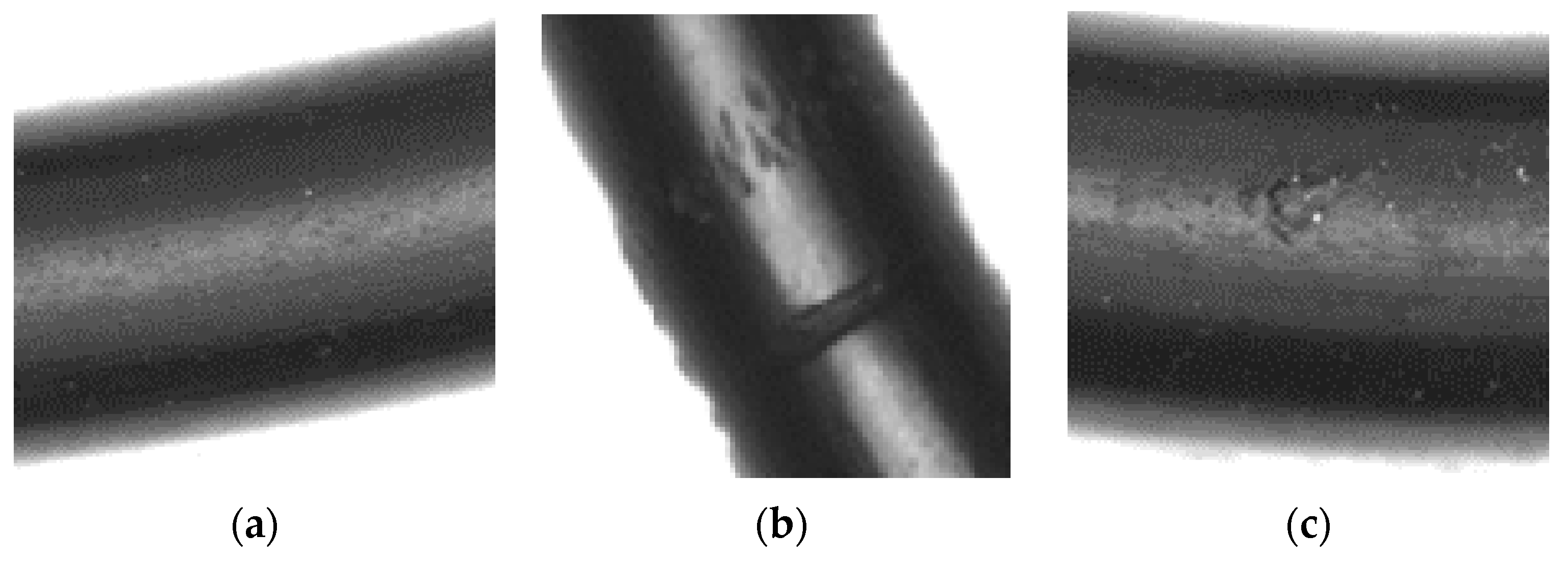
4.1. Defection Detection
4.2. Dimension Measurement
5. Conclusions
Author Contributions
Funding
Institutional Review Board Statement
Informed Consent Statement
Conflicts of Interest
References
- Peng, G.; Zhang, Z.; Li, W. Computer vision algorithm for measurement and inspection of O-Rings. Measurement 2016, 94, 828–836. [Google Scholar] [CrossRef]
- Ho, C.-C.; Lu, J.-J.; Li, P.-C. Development of auto defect inspection system for cell phone silicone rubber gasket. In Proceedings of the 10th International Symposium on Precision Engineering Measurements and Instrumentation (ISPEMI 2018), Kunming, China, 8–10 August 2018. [Google Scholar]
- Husmann, T.; Kreimeier, D. Measurement of radial-axial rolled rings by using image processing and thermography. In Key Engineering Materials; Trans Tech Publ.: Stafa, Switzerland, 2015; pp. 278–283. [Google Scholar]
- Husmann, S.; Husmann, T.; Meier, H. Measurement of rings via image processing during and after radial-axial ring rolling. In Applied Mechanics and Materials; Trans Tech Publ.: Stafa, Switzerland, 2015; pp. 136–143. [Google Scholar]
- Dokken, T.; Dæhlen, M.; Lyche, T.; Mørken, K. Good approximation of circles by curvature-continuous Bézier curves. Comput. Aided Geom. Des. 1990, 7, 33–41. [Google Scholar] [CrossRef]
- Lin, J.-F. Use of Cubic Bézier Curve Approximation of Fourth-Order Bézier Curve. Master’s Thesis, National Chung Cheng University, Chiayi, Taiwan, 2012. [Google Scholar]
- Bézier, P. Courbes et surfaces pour la CFAO. Tech. l’Ingénieur 1992, A1440, 1–18. [Google Scholar]
- Goldapp, M. Approximation of circular arcs by cubic polynomials. Comput. Aided Geom. Des. 1991, 8, 227–238. [Google Scholar] [CrossRef]
- Urbikain, G.; Alvarez, A.; López de Lacalle, L.N.; Arsuaga, M.; Alonso, M.A.; Veiga, F. A reliable turning process by the early use of a deep simulation model at several manufacturing stages. Machines 2017, 5, 15. [Google Scholar] [CrossRef]
- Urbikain, G.; Perez, J.M.; López de Lacalle, L.N.; Andueza, A. Combination of friction drilling and form tapping processes on dissimilar materials for making nutless joints. Proc. Inst. Mech. Eng. Part B J. Eng. Manuf. 2018, 232, 1007–1020. [Google Scholar] [CrossRef]
- Fluid Power Systems—O-Rings—Part 3: Quality Acceptance Criteria; ISO 3601-3:2005; International Organization for Standardization: Geneva, Switzerland, 2005.
- Fluid Power Systems—O-Rings—Part 1: Inside Diameters, Cross-Sections, Tolerances and Designation Codes; ISO 3601-1:2012; International Organization for Standardization: Geneva, Switzerland, 2012.
- Zhang, J. A New 3D Reconstruction Algorithm Based on Photometric Stereo. Master’s Thesis, Northwestern Polytechnical University, Shaanxi, China, 2004. [Google Scholar]
- Suzuki, S. Topological structural analysis of digitized binary images by border following. Comput. Vis. Graph. Image Process. 1985, 30, 32–46. [Google Scholar] [CrossRef]
- Din, I.; Anwar, H.; Syed, I.; Zafar, H.; Hasan, L. Projector calibration for pattern projection systems. J. Appl. Res. Technol. 2014, 12, 80–86. [Google Scholar] [CrossRef] [Green Version]
- Dubrofsky, E. Homography Estimation. Ph.D. Thesis, The University of British Columbia, Kelowna, BC, Canada, 2009. [Google Scholar]
- Douglas, D.H.; Peucker, T.K. Algorithms for the reduction of the number of points required to represent a digitized line or its caricature. Cartogr. Int. J. Geogr. Inf. Geovisualization 1973, 10, 112–122. [Google Scholar] [CrossRef] [Green Version]
- Boehm, W.; Müller, A. On de Casteljau’s algorithm. Comput. Aided Geom. Des. 1999, 16, 587–605. [Google Scholar] [CrossRef]
- Fluid Power Systems—O-Rings—Part 2: Housing Dimensions for General Applications; ISO 3601-2:2016; International Organization for Standardization: Geneva, Switzerland, 2016.
- Aerospace Fluid Systems—O-Rings, Inch Series: Inside Diameters and Cross Sections, Tolerances and Size-Identification Codes—Part 1: Close Tolerances for Hydraulic Systems ISO; ISO 16031-1:2002; International Organization for Standardization: Geneva, Switzerland, 2002.
- Aerospace Fluid Systems—O-Rings, Inch Series: Inside Diameters and Cross-Sections, Tolerances and Size-Identification Codes—Part 2: Standard Tolerances for Non-Hydraulic Systems; ISO 16031-2:2003; International Organization for Standardization: Geneva, Switzerland, 2003.


| Limits of Size for Surface Imperfections for Grade N O-Rings | |||||||
|---|---|---|---|---|---|---|---|
| Surface Imperfection Type | Diagrammatic Representation | Limiting Dimensions | Maximum Limits of Imperfections Grade N O-Rings Cross-Section, d2 | ||||
| >0.8 ≤2.25 | >2.25 ≤3.15 | >3.15 ≤4.50 | >4.50 ≤6.30 | >6.30 ≤8.40 | |||
| Excessive trimming (radial tool marks not allowed) |  | n | Trimming is allowed provided the dimension n is not reduced below the minimum diameter d2 for the O-Ring. | ||||
| Flow marks (radial orientation of flow marks is not permissible) |  | v | 1.50 | 1.50 | 6.50 | 6.50 | 6.50 |
| k | 0.08 | 0.08 | 0.08 | 0.08 | 0.08 | ||
| Non-fills and indentations (including parting line indentations) |  | w | 0.60 | 0.80 | 1.00 | 1.30 | 1.70 |
| t | 0.08 | 0.08 | 0.08 | 0.10 | 0.13 | ||
| Name | Specification and Parameter |
|---|---|
| Trademark and model | VR-3100 |
| Magnification | 12× |
| FOV(field of view) | 24 × 18 mm2 |
| Resolution | 1024 × 768 |
| Working distance | 75 mm |
| Pixel size | 23.4375 × 23.4375 m2 |
| Repeatability (Vertical) | 0.5 μm |
| Repeatability (horizontal) | 1 μm |
| SIC (Size Identification Code) | Internal Diameter d1 (mm) | Cross-Section d2 (mm) | ||
|---|---|---|---|---|
| Min. | Max. | Min. | Max. | |
| −005 | 2.44 | 2.69 | 1.70 | 1.85 |
| −006 | 2.77 | 3.02 | 1.70 | 1.85 |
| −007 | 3.56 | 3.81 | 1.70 | 1.85 |
| −008 | 4.34 | 4.60 | 1.70 | 1.85 |
| −009 | 5.16 | 5.41 | 1.70 | 1.85 |
| −010 | 5.94 | 6.20 | 1.70 | 1.85 |
| −011 | 7.52 | 7.77 | 1.70 | 1.85 |
| −012 | 9.12 | 9.37 | 1.70 | 1.85 |
| −013 | 10.69 | 10.95 | 1.70 | 1.85 |
| −014 | 12.29 | 12.55 | 1.70 | 1.85 |
| −015 | 13.87 | 14.12 | 1.70 | 1.85 |
| −016 | 15.47 | 15.72 | 1.70 | 1.85 |
| −017 | 17.04 | 17.30 | 1.70 | 1.85 |
| −018 | 18.64 | 18.90 | 1.70 | 1.85 |
| −019 | 20.19 | 20.50 | 1.70 | 1.85 |
| −020 | 21.79 | 22.10 | 1.70 | 1.85 |
| −021 | 23.36 | 23.67 | 1.70 | 1.85 |
| −022 | 24.97 | 25.27 | 1.70 | 1.85 |
| −023 | 26.54 | 26.85 | 1.70 | 1.85 |
| Image Index | ||||
|---|---|---|---|---|
| 1 | 2 | 3 | ||
| SIC | −017 |  |  |  |
| −018 |  |  |  | |
| −019 |  |  |  | |
| −020 |  |  |  | |
| True Condition | |||
|---|---|---|---|
| Positive | Negative | ||
| Predicted Outcome | Positive | 160 | 11 |
| Negative | 0 | 149 | |
| Accuracy | 96.56% | ||
| Precision | 93.57% | ||
| Recall | 100% | ||
| True Condition | |||
|---|---|---|---|
| Positive | Negative | ||
| Predicted Outcome | Positive | 160 | 0 |
| Negative | 0 | 160 | |
| Accuracy | 100% | ||
| Precision | 100% | ||
| Recall | 100% | ||
| Unit: mm | Methods of Measurement | ||
|---|---|---|---|
| Name of Database | Bp | A | C |
| DVT | 0.01401 | 0.04627 | 0.47170 |
| DSI | 0.04606 | 0.07764 | 0.48437 |
| DSP | 0.03703 | 0.13972 | 0.87662 |
| Unit: mm | Methods of Measurement | ||
|---|---|---|---|
| Name of Database | Bp | A | C |
| DVT | 0.00741 | 0.01657 | 0.03544 |
| DSI | 0.03424 | 0.04591 | 0.05424 |
| DSP | 0.02697 | 0.04145 | 0.29591 |
Publisher’s Note: MDPI stays neutral with regard to jurisdictional claims in published maps and institutional affiliations. |
© 2021 by the authors. Licensee MDPI, Basel, Switzerland. This article is an open access article distributed under the terms and conditions of the Creative Commons Attribution (CC BY) license (http://creativecommons.org/licenses/by/4.0/).
Share and Cite
Yang, F.-S.; Ho, C.-C.; Chen, L.-C. Automated Optical Inspection System for O-Ring Based on Photometric Stereo and Machine Vision. Appl. Sci. 2021, 11, 2601. https://doi.org/10.3390/app11062601
Yang F-S, Ho C-C, Chen L-C. Automated Optical Inspection System for O-Ring Based on Photometric Stereo and Machine Vision. Applied Sciences. 2021; 11(6):2601. https://doi.org/10.3390/app11062601
Chicago/Turabian StyleYang, Fu-Sheng, Chao-Ching Ho, and Liang-Chia Chen. 2021. "Automated Optical Inspection System for O-Ring Based on Photometric Stereo and Machine Vision" Applied Sciences 11, no. 6: 2601. https://doi.org/10.3390/app11062601