1. Introduction
Gradient boosted tree (GBT) models [
1] remain the state-of-the-art for many “shallow” learning tasks that are based on structured, tabular data sets [
2,
3,
4]. Such tasks are often still found in high-stakes decision making domains, such as medical decision making [
5,
6,
7,
8]; justice and law [
9,
10]; financial services [
11,
12,
13]; and defence and military intelligence [
14]. In these and similar domains, there is a high burden of accountability for decision makers to explain the reasoning behind their decisions. This burden only increases with the introduction of machine learning (ML) into decision making processes [
15]. So, the very high accuracy and ease of use of GBT models is not enough to encourage their adoption because GBT models also typify the “black box” problem of uninterpretability. Hence, research in interpretable machine learning (IML) and explainable artificial intelligence (XAI) has emerged to overcome these barriers to adoption.
Deriving explanations from the complex structure of GBT models (as an ensemble of decision trees) has remained an open challenge. Gradient-based attribution methods that are used to explain deep learning (DL) models and neural networks are unsuitable here because the internal sub-units of a GBT model are non-parametric and non-differentiable decision nodes. The available IML and XAI methods have several disadvantages.
IML methods can be used to facilitate the interpretation of a GBT model, as well as other types of decision tree ensemble, also known as decision forests (DFs). These methods generate a cascading rule list (CRL) as an inherently interpretable proxy model. First, a very large set of candidate classification rules (CRs) is generated. The defragTrees [
16] and inTrees [
17] methods achieve this by extracting all possible CRs from the decision trees in the DF. Bayesian rule lists (BRLs) [
18] use a different approach, which is to mine the rules directly from the training data. For all three methods, the candidate set of CRs is then merged or pruned using, e.g., some Bayesian formulation into the final CRL. One disadvantage with this approach is the very high computational and memory cost of exploring the combinatorial search space of candidate CRs. Another is imperfect fidelity, which means that the proxy does not always agree with the reference model’s classification. This is a consequence of the proxy’s simplification of the complex behaviour of the black box reference model. Disagreement between the two results in a failure to explain the reference model.
Currently available XAI methods for explaining GBT are the so called model-agnostic methods. Methods include locally interpretable model-agnostic explanations (LIMEs) [
19], Shapley additive explanations (SHAP) [
20], local rule-based explanations (LORE) [
21], and anchors [
22]. These general purpose methods are said to explain any model. This flexibility is achieved by using a synthetic data set to probe the reference black box model and infer a relationship between its inputs and outputs. However, these methods are disadvantaged because there is no introspection of the reference model or target distribution, which is thought to be essential for reliable explanations [
23,
24]. Furthermore, the explanations can exhibit variance because of the non-deterministic data generation [
25,
26]. High variance results in dissimilar explanations for similar instances. They can also be fooled by adversarial examples [
27]. Furthermore, the synthetic data place too much weight on rare and impossible instances [
28,
29,
30].
Recent contributions [
31,
32] present model-specific XAI approaches that probe DF internals and generate a single CR as an explanation. Thus, these newer methods overcome the combined disadvantages of prior work and have been shown to outperform the model-agnostic XAI methods and CRL-based IML methods on other classes of DF. Namely, the random forest [
33] and AdaBoost [
34] models. Hence, there still remains a gap in the literature for model-specific explanation methods that target GBT models. This research addresses that gap.
In this paper, we present Gradient Boosted Tree High Importance Path Snippets (gbt-HIPS), a novel, model-specific algorithm for explaining GBT models. The method is validated against the state-of-the-art in a comprehensive experimental study, using nine data sets and five competing methods. gbt-HIPS offered the best trade off between coverage (0.16–0.75) and precision (0.85–0.98) and was demonstrably guarded against under- and over-fitting. A further distinguishing feature of our method is that, unlike much prior work, our explanations also provide counterfactual detail in accordance with widely accepted best practice for good explanations.
The remainder of this paper is set out as follows:
Section 2 presents gbt-HIPS, our novel algorithm for generating explanations of GBT classification;
Section 3 describes our experimental procedures;
Section 4 discusses the results; and
Section 5 concludes the paper with some ideas for future research.
2. The Gbt-HIPS Method
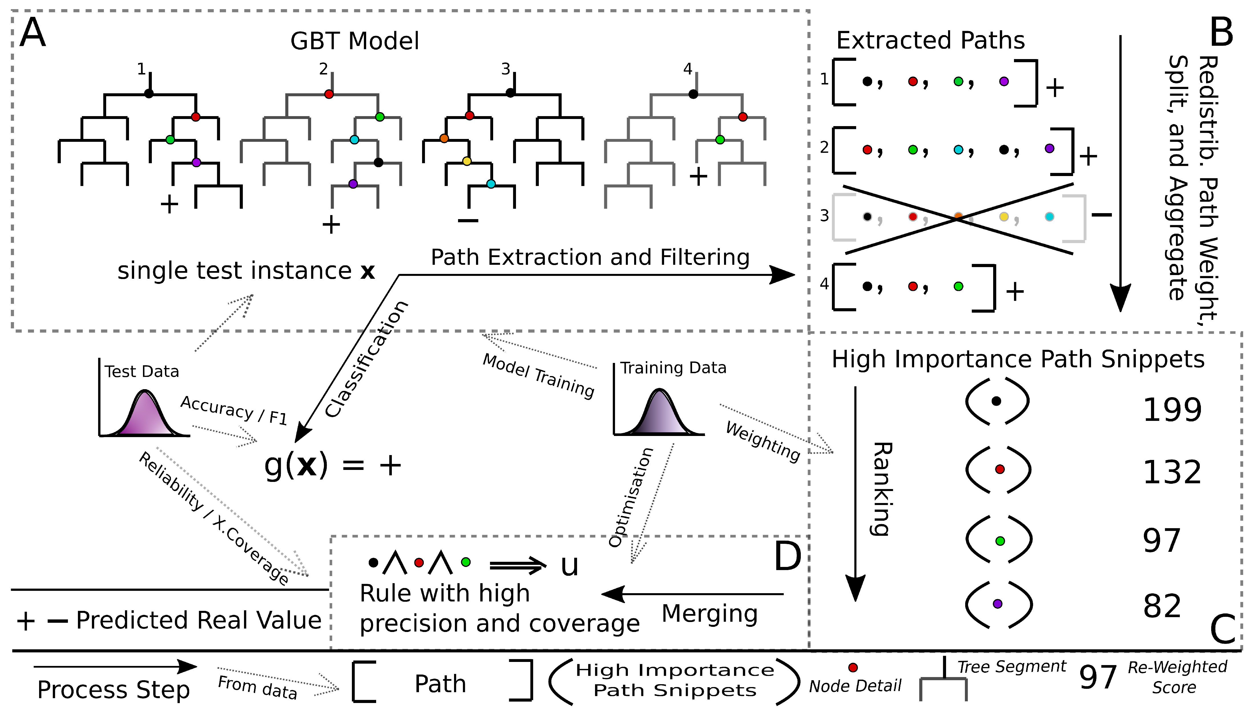
This section presents Gradient Boosted Trees High Importance Path Snippets (gbt-HIPS) method in detail. Each step is illustrated in the conceptual diagram in
Figure 1 and detailed in the following sections.
The design of gbt-HIPS takes into consideration Miller’s key principles [
35]. To the best of our knowledge, very few prior works have responded to those insights so directly, with the exception of [
31,
32]. The “model of self” principle suggests that, in order to be a true representation of the model’s internal logic, the explanation must, in some way, be formed from the model internals. This idea is echoed in the four axioms given in [
23], e.g., “Explanation without introspection is not explanation.” The form of explanation is a single CR extended with counterfactual detail, as is expected by Miller’s “contrastive” principle. The CR form naturally aligns with the other key principles of “selectivity” and “minimal completeness.” These are satisfied when the rule contains the right combination of antecedent terms to cover a non-trivial volume of the input space, while each individual term is necessary to ensure maximal rule precision. The counterfactual detail is the loss of precision that arises when any single antecedent term is violated. This fuzzy counterfactual is a necessary adaptation for data that contains any continuous variables and, in fact, provides much more information than a discrete change of class label. For full details, refer to [
31].
The gbt-HIPS algorithm follows a greedy, breadth-first, heuristic search. The first step is to set the CR consequent as the black box model’s output. Thus, by design, the CR will always agree with the black box for the explanandum. Then, candidate decision nodes are extracted from the decision trees in the ensemble with two filtering steps unique to this research. The importance of each decision node (and therefore its opportunity to be included in the rule antecedent) is calculated by means of a statistically motivated procedure, based on relative entropy. These weighted decision nodes are referred to as path snippets. The resulting snippets are merged into a final rule according to a simple, greedy heuristic. The following paragraphs describe the process in full detail.
2.1. Path Extraction and Filtering
The first step is to extract the decision path of the explanandum instance from every decision tree in the GBT model g. This design choice means that, unlike in IML methods, the rest of the model is ignored when generating the explanation for the given classification event . This filtering reduces the size of the search logarithmically and is justified because there is only one possible path for down each tree. So, none of the other paths contribute to the final output.
In the multi-class case, GBT models consist of K one-vs-all binary logistic classifiers. So, classification is normally modified such that the winning class is determined by the kth classifier that has the largest positive value. gbt-HIPS uses only paths from this kth classifier.
Path extraction simply records the detail at each decision node as it is traversed by the explanandum instance on its way to a terminal node. The decision path consists of this set of decision nodes along with the real-valued output from the terminal node. Recall that GBT uses regression trees, whose aggregated outputs make a log odds prediction. The extracted paths are then filtered to retain only the paths whose terminal node output has the same sign as the ensemble output (always positive for multi-class settings but could be either sign in binary settings). This stage of filtering is justified because those paths that do not agree with the overall ensemble “lose the election.” The decision nodes in the retained paths contain all the information about the model’s output. The excluded paths are expected to capture noise, or perhaps attributes that are more strongly associated with the alternative class.
2.2. Redistribute Path Weight, Split the Paths, and Aggregate the Nodes
This second step is critical for assigning importance scores to the decision nodes. The path’s weight is the absolute value returned by the path’s terminal node. The path weights represent each individual tree’s contribution to the log odds prediction and must be fairly distributed over each decision node in the path. The redistribution must take into account the node order in the originating path as well as the predictive power of the node itself. The KL-divergence, also known as relative entropy, is ideal for this purpose because it measures information gained if a new distribution (
P) is used, instead of a reference distribution (
). The KL-divergence is calculated as follows:
where
P is the distribution of class labels for instances that reach a given node in the path and
is the distribution that reaches the previous node in the path. In the case of the root node, which is first in the path,
is simply the prior distribution. Here, the quantities are estimated using the training set or any other large i.i.d. sample. Once the relative entropy for the last decision node in the path is evaluated, the values for the entire path are normalised, such that their total is equal to that of the path weight.
The paths are then disaggregated into the individual, weighted decision nodes and stored in a key-value dictionary, with the decision nodes as keys and the redistributed path weights as values. The weights for identical nodes are aggregated by summation as they enter the dictionary. While this operation is straightforward for nodes that represent discrete or categorical features, there is a complication with nodes that act on continuous features that is a natural consequence of GBT training. On each training iteration, the instances are re-weighted, which alters the target distribution. See [
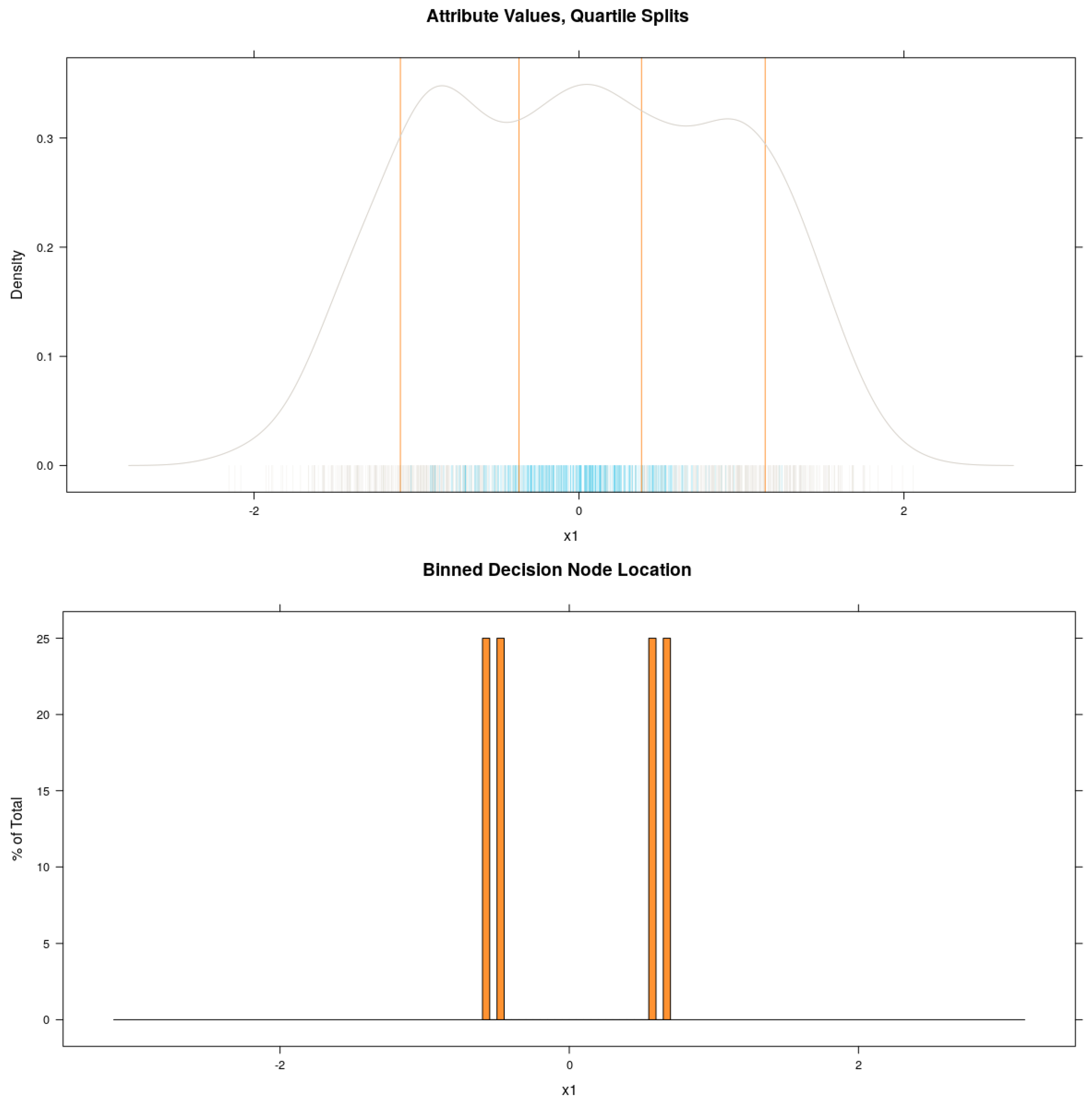
1] for further details. A further perturbation occurs in the very common stochastic GBT variant. Stochastic GBT takes random samples of training instances on each iteration, in addition to the aforementioned re-weighting. Hence, when a new decision tree is induced over the modified distribution, the exact location at which continuous features might be partitioned can move from one iteration to the next in a non-deterministic manner. That is to say, many unique values may all represent the same decision boundary. Competing methods (such as LIME, Anchors, SHAP and the IML models) avoid this problem by preprocessing the continuous features into arbitrary, quartile bins. There are several problems with this approach, not least of which is a loss of information because the quartile bin medians are very unlikely to align with the optimal boundary values. gbt-HIPS instead delegates this discretisation step to the GBT model training. More specifically, it is the information theoretic step of decision tree induction that determines the location of each split in the continuous variables. gbt-HIPS applies a simple binning function to all the extracted decision node boundary values for each continuous feature.
This idea is illustrated in
Figure 2. In this toy example, the data set shown has one feature,
and two classes. The negative class − (blue) is found mostly around the middle of the range of
and is completely enclosed by the positive class + (grey). A GBT model is trained for 1000 iterations using decision trees with
, allowing each tree to find two boundary values. The effect of having a freshly perturbed training distribution on each iteration is that each decision node represents a sample from the approximate locations of the optimal boundary values. The resulting decision node boundary values are binned with a simple histogram function. Thus, it is possible to find a very small number of near optimal boundary values to include in the explanations, removing the aforementioned unique value problem. It is clear from
Figure 2 that the decision boundary bin medians of the model (shown in the lower panel) align very closely with the cluster boundaries. On the other hand, quartile bin medians that sit half-way between the quartile boundaries (superimposed on the kernel density plot, top panel) tend to split clusters in half or simply appear at arbitrary locations relative to the distribution. This simple example demonstrates that preprocessing by quartile binning does not lead to optimal candidate boundary values for the explanations while gbt-HIPS’s post-processing binning does.
2.3. Ranking
At this point, the individual decision nodes are separated from their originating path and each decision has an aggregated weight. We refer to their new state as path snippets. The dictionary of unique path snippets created in the previous step is simply sorted by weight, in descending order. Ranking is essential for avoiding an exhaustive search in the next step, because the ordering controls the path snippets’ opportunity to be included in the candidate explanation. It is reasonable at this point to filter out the path snippets with the smallest aggregated weight using a top n or top hyper-parameter, as it will shorten the step that follows.
2.4. Merging and Pruning
The final step generates the CR-based explanation using a breadth first, greedy, heuristic search of the path snippets. Before the search commences, the first step is to set the rule consequent as the GBT model’s classification of the explanandum instance . This step guarantees local accuracy. The search then begins from , the “null” rule that has an empty antecedent and maximum coverage. The first path snippet, at the top of the sorted dictionary, is appended to the rule’s antecedent. The reliability on the training data is evaluated and this value stored. Then, one at a time in turn, path snippets from the sorted dictionary are added as candidate antecedent terms. If the union improves the reliability, the snippet is retained in the rule. If not, the snippet is simply discarded. In both cases snippets are removed from the dictionary.
To further reduce the number of iterations, any path snippets are deleted from the ranked list if they contain boundary values of continuous features that fall outside the current coverage region. That is, coverage is forced to decrease monotonically. These steps, merging a path snippet and pruning the dictionary, iterate until a target reliability threshold is met or the list is exhausted, as illustrated in Algorithm 1.
| Algorithm 1 Rule Merging |
- 1:
procedure RuleMerge() ▷ Inputs: model, training data, explanandum, sorted map, target reliability. - 2:
▷ Candidate set of antecedent terms - 3:
▷ Prior reliability. - 4:
while and length do - 5:
▷ Append top ranking path snippet. Partition only covered instances. - 6:
if then - 7:
▷ Path snippet added to rule. - 8:
- 9:
▷ Remove top snippet. Reset indices. - 10:
return
|
After rule merging completes, the candidate set of antecedent terms
is returned, forming the final candidate rule. This candidate is pruned of extraneous terms in a process that also generates the counterfactual detail, while enforcing minimal completeness, as required by Miller’s principles of explanation [
35]. The inclusion of extraneous terms can occur because the greedy heuristic only enforces a monotonic increase in reliability. Thus, terms that increase performance only very slightly may be included. Furthermore, some antecedent terms are rendered redundant through interaction with terms that are added subsequently. These non-optimal side-effects are to be expected with greedy, heuristic algorithms. Therefore, the pruning step iterates through the “point changes”, removing any antecedent terms that are found to be extraneous. A point change is defined as the reversal of the inequality constraint of a single antecedent term. Therefore, point changes represent a set of “adjacent spaces” to that hyper-cube (or half-space) of the input space that is covered by the rule. Adjacent spaces are outside the hyper-cube by one axis-aligned step across a single rule boundary. To determine whether an antecedent term is extraneous, the reliability is evaluated on the training instances covered by each adjacent space. If reliability decreases by <
(a user-defined parameter) inside an adjacent space, that antecedent term can be removed from the rule. The result is a shorter rule that has a greater coverage and whose reliability lies within the user-defined tolerance of the unpruned candidate’s reliability.
2.5. Output
The final output is the rule, together with estimates of any requested statistics evaluated for the training set or other i.i.d. sample. Estimates of precision for each of the adjacent spaces convey the counterfactual detail. This formulation should aid the end user in validating the importance of each antecedent term.
An example of this output is given in
Table 1 and is taken from the adult data set that is freely available from the UCI Machine Learning Repository [
36]. In this classification task, models are trained to predict whether an individual has an annual income greater than or less than/equal to
K using a set of input features related to demographics and personal financial situation. The explanandum instance here was selected at random from a held out test set. The GBT model classified this instance as having an income less than or equal to
K per annum. The explanation column shows the final CR, one row per term. This CR covers
of training samples with a precision of
(instances in the half-space that correctly receive the same classification). These boundary values include only the two attributes: (log) capital gain is less than 8.67 and marital status is not equal to married-civ, giving a very short rule that is trivial for human interpretation. The contrast column contains the counterfactual detail, which is the change in the rule’s precision when the inequality in each antecedent term is reversed, one at a time, i.e., substituting ≤ for >, or ≠ for =. Reversing either one of these boundary values in this way (thus exploring the input space outside the enclosed half-space) creates a CR with either the opposite outcome or a result that is worse than a random guess if controlling for the prior distribution. This is, therefore, a very high quality explanation.
3. Materials and Methods
The work described in the coming sections is reproducible using code examples in our github repository
https://tinyurl.com/yxuhfh4e (5 March 2021).
3.1. Experimental Design
The experiments were conducted using both Python 3.6.x and R 3.5.x environments, depending on the availability of open-source packages for the benchmark methods. The hardware used was a TUXEDO Book XP1610 Ultra Mobile Workstation with Intel Core i7-9750H @ 2.60–4.50 GHz and 64GB RAM using the Ubuntu 18.04 LTS operating system.
This paper follows exactly the experimental procedures described in [
31,
32], which adopt a functionally grounded evaluation [
37]. The use of this category is well justified because the present research is a novel method in its early stages, and there is already good evidence from prior human-centric studies demonstrating that end users prefer high precision and coverage CR-based explanations over additive feature attribution method (AFAM) explanations [
21,
22]. The efficacy of CR-based explanations is also already well-established by IML models [
7,
24,
38,
39]. Functionally grounded studies encourage large-scale experiments. So, this research will compare the performance of gbt-HIPS with five state-of-the-art methods on nine data sets from high-stakes decision-making domains.
The aforementioned precedents [
21,
22] measure the mean precision and coverage for the CR-based explanations generated from a held out set of instances that were not used in model training. Those precedents found that coverage and precision were effective as proxies to determine whether a human user would be able to answer the fundamental questions: “does a given explanation apply to a given instance?” and “with what confidence can the explanation be taken as valid?”
The experimental method uses leave-one-out (LOO) evaluation on held out data to generate a very large number of test units (explanations) in an unbiased manner from each data set. This approach is better suited to the XAI setting because every explanation is independent of the training set, and independent of the set used to evaluate the statistics of interest. Each data set was large enough that any inconsistencies in the remaining evaluation set were ignorable.
Aforementioned related work indicates that individual explanations can take between a fraction of a second and a few minutes to generate. This timing was confirmed in a pilot study, prior to the forthcoming experimental research. To balance the need for a large number of explanations against the time required to run all the tests, the experimental study will generate 1000 explanations or the entire test set, whichever number is smaller.
3.2. Comparison Methods and Data Sets
gbt-HIPS produces CR-based explanations. Direct comparisons are possible against other methods that either output a single CR as an explanation, or a rule list from which a single CR can be extracted. Readers that have some familiarity with XAI may question the omission of LIME [
19] and SHAP [
20] from this study since they are two of the most discussed explanation methods to date. However, as the authors of [
20] make clear, these are AFAM and, therefore, of an entirely different class. There is no straightforward way to compare explanations from different classes as prior works have demonstrated [
21,
22]. For example, there is no way to measure the coverage of an AFAM explanation over a test set, whereas for a CR the coverage is unambiguous. Fortunately, Anchors [
22] has been developed by the same research group that contributed LIME. Anchors can be viewed as a CR-based extension of LIME and its inclusion into this study provides a useful comparison to AFAM research. In addition to Anchors, LORE [
21] is included, as another per-instance, CR-based explanation method. These are the only such methods that are freely available as open-source libraries for Python and R development environments.
We also included three leading CRL-based interpretable machine learning (IML) methods into the study design. When using CRL models, the first covering (or firing) rule is used to classify the instance and, thus, is also the stand-alone explanation. If there is no covering rule, the default rule is fired. This
null rule simply classifies using the prior class majority. For the purposes of measuring rule length, a firing null rule has a length of zero. All selected methods are detailed in
Table 2.
The nine data sets selected for this study have been carefully selected to represent a mix of binary and multi-class problems, to exhibit different levels of class imbalance (no artificial balancing will be applied), to be a mixture of discrete and continuous features, and to be a contextual fit for XAI (i.e., credit and personal data) where possible. The data sets are detailed in
Table 3. All are publicly available and taken from the UCI Machine Learning Repository [
36] except lending (Kaggle) and rcdv (ICPSR;
https://tinyurl.com/y8qvcgwu (30 October 2019)). Three of these data sets (adult, lending and rcdv) are those used in [
22] and, therefore, align with precedents and provide direct comparisons to state-of-the-art methods Anchors and LIME. The exceptionally large lending data set has been subsampled. The number of instances in the original data set is 842,000 and was downsampled to
for these experiments. Training and test data sets were sampled without replacement into partitions of size 70 and 30% of the original data set.
3.3. Quantitative Study
There is a very strong case that coverage and precision are not appropriate quality metrics for explanations-based research [
31,
32]. Coverage is trivially maximised by critically under-fitting solutions. For example, the
null rule
(all inputs result in the given output) is critically under-fitting, yet scores
for coverage. Precision, conversely, is trivially maximised by critically over-fitting solutions. For example, the “tautological” rule
(the unique attributes of the explanandum result in the given output) is critically over-fitting yet scores
for precision.
These metrics are absolutely ubiquitous throughout the ML, statistical and data mining literature, which might explain their continued application in XAI experimental research. This research prefers
reliability and
exclusive coverage, first proposed in [
31], because they penalise any explanations that approach the ill-fitting situations described above. However, to assist the user in understanding the utility of these novel metrics, both sets of results (novel and traditional) are presented. The rule length (cardinality of the rule antecedent) is also measured. These metrics are supplemented by the reliability floor and the rule length floor. The reliability floor is the proportion of evaluated explanations that clear the threshold of
reliability, and the rule length floor is the proportion of explanations with a length greater than zero. Both of these supplementary statistics are useful for quantifying the prevalence of over- and under-fitting. These pathological behaviours can easily be masked when only looking at aggregate scores (means, mean ranks, etc.). We will also present the fidelity scores that reveal when methods/proxy models do not agree with the black box reference model.
The computational complexity will be compared using the mean time (sec) to generate a single explanation. The authors of [
19,
22] state that their methods take a few seconds to a few minutes to generate an explanation. We conjecture that something less than thirty seconds would be considered acceptable for many Human–in–the–Loop processes because each explanation requires further consideration prior to completion of a downstream task. Consideration and completion steps would likely be much longer than this simple time threshold.
Significance (where required) shall be evaluated with the modified Friedman test, given in [
40]. The Friedman test [
41] is a non-parametric equivalent to ANOVA and an extension of the rank sum test for multiple comparisons. The null hypothesis of this test is that the mean ranks for all groups are approximately equal. In these experiments, the groups are the competing algorithms. The alternative hypothesis is that at least two mean ranks are different.
On finding a significant result, the pairwise, post-hoc test can be used to determine which of the methods perform significantly better or worse than the others. It is sufficient for this study to demonstrate whether the top scoring method was significantly greater than the second place method. Note, however, that the critical value is applied as if all the pairwise comparisons were made. The critical value for a two-tailed test with the Bonferroni correction for six groups is . The winning algorithm is formatted in boldface only if the results are significant.
4. Discussion
This section presents the main results of the experimental research. Supplementary results are available from our github repository
https://tinyurl.com/yxuhfh4e (5 March 2021). Note, all the Friedman tests yielded significant results. Consequently, these results are omitted and we proceed directly to the pairwise, post-hoc tests between the top two methods. These post-hoc tests will help to determine if there is an overall leading method.
4.1. Fidelity
Fidelity (the agreement rate between the explanations’ consequent and the reference model’s output), is given in
Table 4. Only gtb-HIPS and Anchors are guaranteed to be locally accurate by means of their algorithmic steps. Unfortunately, it was not possible to collect the fidelity scores for the LORE method. The computation time of the (very long-running) method, which makes it prohibitive to re-run the experiments. However, the fidelity of LORE is listed in the originating paper [
21] as
for the adult data set,
for the german data set, and
for a third data set not used in this investigation. LORE is assumed to reach this level of fidelity for other data sets used in these experiments.
It must be noted that poor fidelity with the black box model is a critical flaw. An explanation in the form of a classification rule is not fit for purpose if the consequent does not match the target class. On this point, there can be little debate because a key requirement, local accuracy, is violated. On the other hand, the tolerance for anything less than perfect fidelity is a domain-specific question. This tolerance will depend on the cost or inconvenience of failing to explain any given instance. So, we make only the following assertion as to what is an acceptable score: it would be surprising to find levels as low as permissible in critical applications. At this level, one in ten explanations is unusable.
4.2. Generalisation
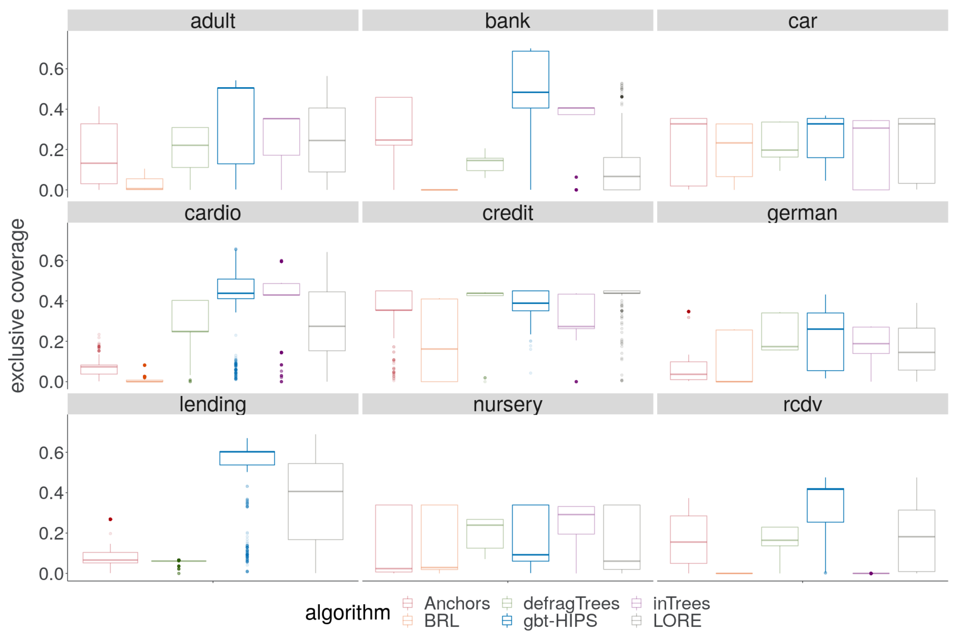
Good performance on the exclusive coverage metric indicates that the explanations generalise well to new data. Such rules cover a large proportion of data from the target distribution without covering large numbers of instances that the black box classified differently than the explanandum instance.
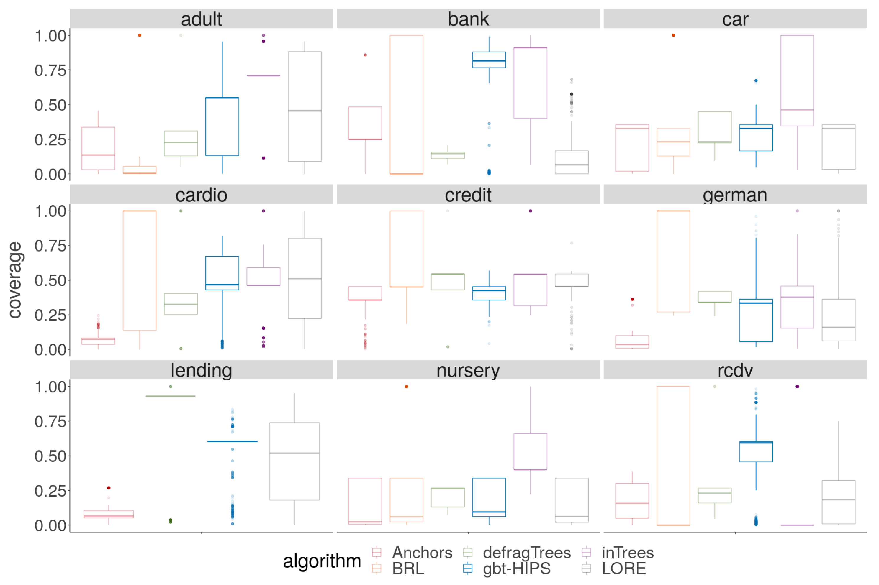
A cursory visual inspection the coverage (
Figure 3) does not reveal any obvious pattern. While there is no overall winning algorithm for coverage, BRL and inTrees are each strongly in the lead for three out of the nine data sets, and gbt-HIPS for two of the remaining three data sets. On the other hand, visual analysis of the exclusive coverage score distribution (
Figure 4) shows that gbt-HIPS is often leading or a close runner-up. The lead that BRL had for simple coverage is completely forfeit. In fact BRL has the lowest exclusive coverage for five out of nine data sets. Furthermore, the inTrees method no longer has the lead in any data set, except for nursery under the exclusive coverage measure. The tabulated mean and mean ranks of these data (in the
supplementary materials) support this visual analysis and show that gbt-HIPS takes the lead for six out of the nine data sets. This result suggests that BRL and inTrees generate explanations that are too general, while gbt-HIPS explanations are robust. This diagnosis is borne out by results from the rule length floor statistic (to follow).
Significance tests between the top two ranking methods are shown in
Table 5. gbt-HIPS ranked first on five data sets, joint first (no significant difference between first and second) on the car data set, second on the german data set, and third out of six methods on the remaining two data sets, making gbt-HIPS the very clear lead.
4.3. Reliability
Good performance on the reliability metric indicates that, for the target distribution, a high proportion of instances covered by the explanation will receive the same classification from the black box model as was given to the explanandum. At the same time, the end user can be certain that the rule does not cover a trivially small region of the input space.
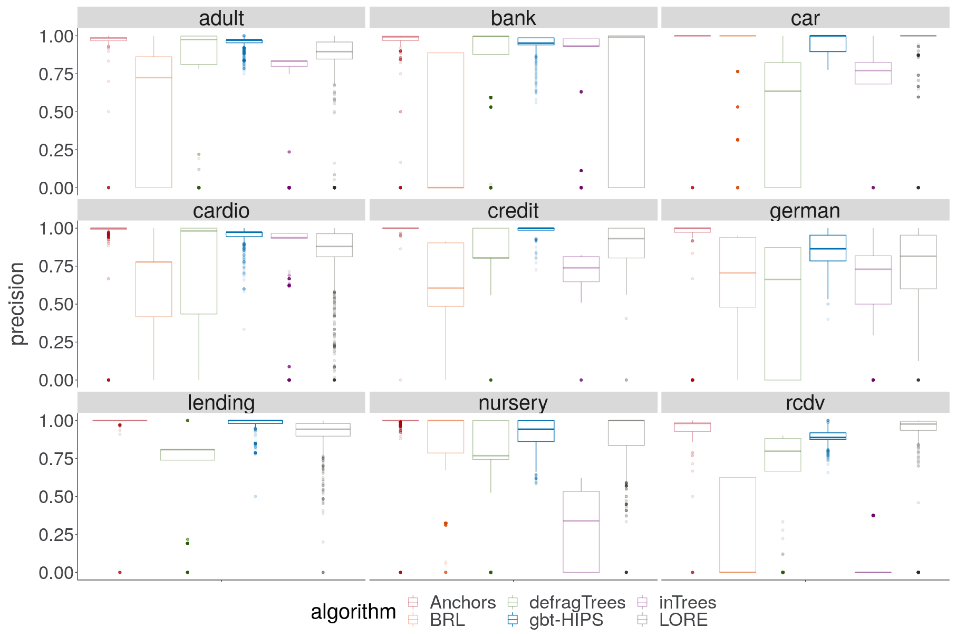
A cursory visual inspection of the precision (
Figure 5) demonstrates the trade-off between precision and coverage. The BRL, inTrees and defragTrees methods that had scored relatively well for coverage do not deliver state-of-the-art precision on any data set. Both precision and reliability (
Figure 6) score distributions show that Anchors and gbt-HIPS vie for first position over almost all of the data sets. Anchors appears to have a slight advantage for precision while gbt-HIPS appears to do better for reliability. The placement is often so close that it requires recourse to the tabulated results (
supplementary materials) and the significance tests to be certain of the leading method.
The results of hypothesis tests of the pairwise comparisons for the top two ranking methods are shown in
Table 6. The tests seem to show that Anchors is leading for reliability on three out of the nine data sets, joint first (no significant difference between first and second place) on a further two data sets, and second on a further two data sets. gbt-HIPS appears to be the second place method, leading on two data sets, and joint first on a further three data sets. These results, it seems, are inconsistent with the tabulated and visualised mean scores for reliability.
These inconsistencies are, unfortunately, an artefact of the choice of significance test, which is non-parametric and, therefore, insensitive to outliers. Specifically, the long tail of under-fitting instances visible as colour saturated dots in the lower parts of each facet of
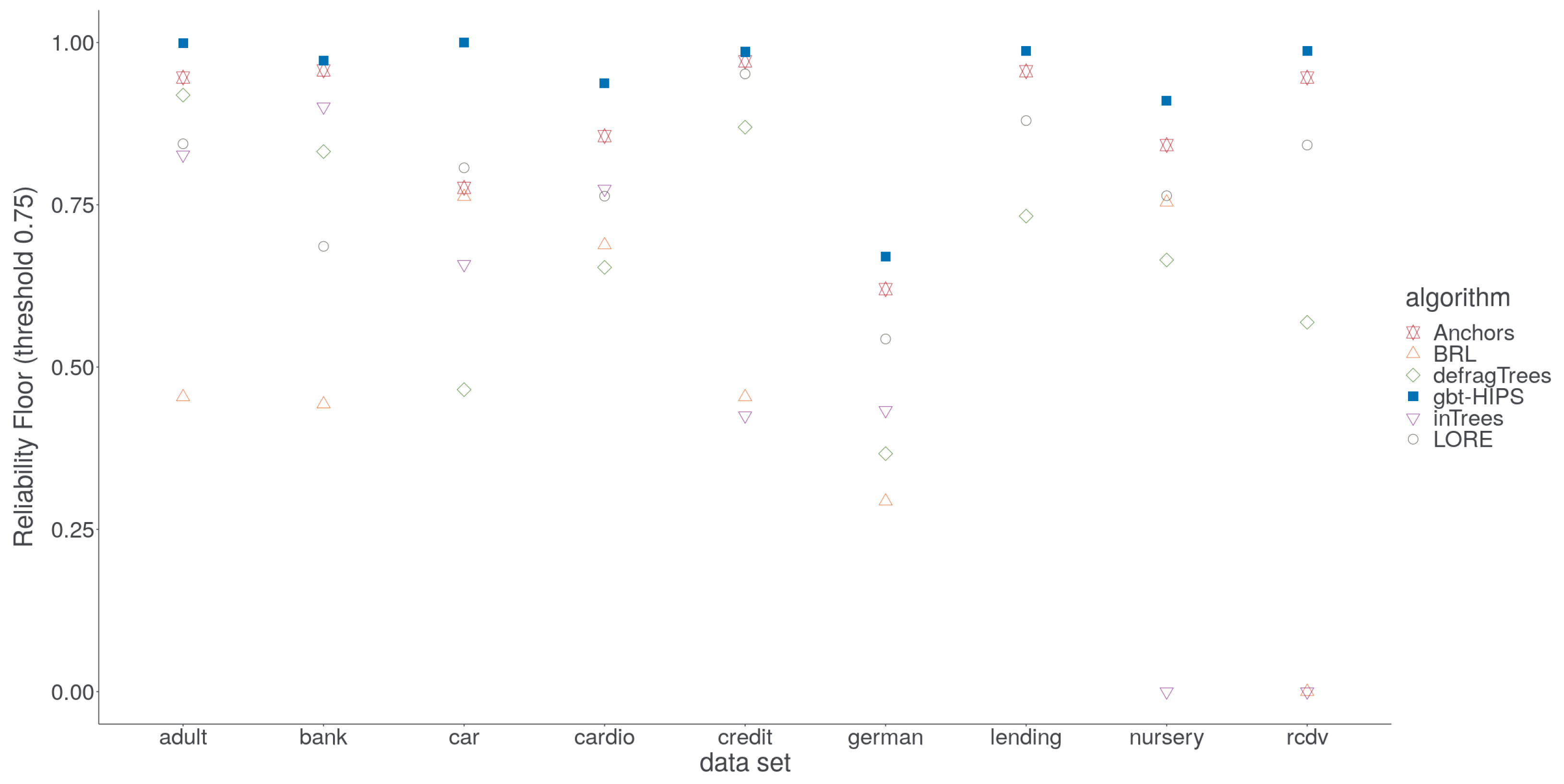
Figure 6. For gbt-HIPS, instead almost the entire set of scores occupies a narrow band near to the upper bound for reliability. It is for this reason that the reliability floor statistic (
Figure 7) is so enlightening. The reliability floor quantifies the propensity to over-fit by measuring the proportion of explanations in the test set that scored above the threshold. Over-fitting explanations are too granular and cover too few instances. Furthermore, a significant number of explanations score zero, demonstrating a critical over-fit. That is, an explanation that covers only the explanandum but not a single instance in the held out set. gbt-HIPS leads on all nine data sets for reliability floor. The reliability floor scores are presented visually in
Figure 7 and tabulated in the
supplementary materials.
4.4. Interpretability
While antecedent length is not an absolute measure, it can be used to compare the relative understandability of CR-based explanations. Significance tests do not form a part of this analysis for the following reason. Even though short rules are the most desirable, a score of zero length (the null rule) is highly undesirable and a sign of under-fitting. The significance test, based on mean ranks of rule lengths (in ascending order) will reward methods with this pathological condition. So, rather than fabricating a new mode of testing, this research relies on the evidence of the visual analysis, and the rule length floor statistic. Anchors and gbt-HIPS are guaranteed never to return a zero length rule via their algorithmic steps. All of the globally interpretable methods, on the other hand, can return the zero length null rule if none of the rules in their list are found to cover the explanandum. It would be highly unexpected for LORE to return a null rule but there is no formal guarantee of this behaviour and, very occasionally, it does occur.
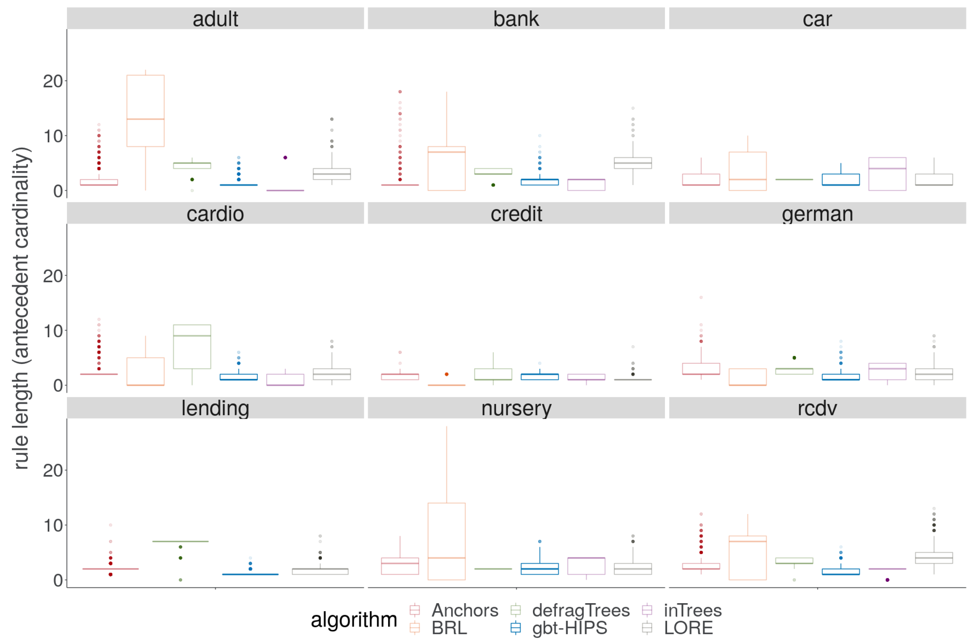
On reviewing the rule length results visually in
Figure 8, it is encouraging to note that gbt-HIPS never generates either the longest rules or suspiciously short rules. Interestingly Anchors, LORE and gbt-HIPS track one another (very approximately) for mean rule length (
supplementary materials) over all the data sets, which might suggest some level of commonality in their outputs. The BRL method, on the other hand, generates the longest rules for four out of five data sets. The defragTrees method generates the longest rules on a further two. In these cases, the rule lengths measured suggest that a large number of instances are explained by rules that are some way down the CRL, resulting in concatenation. The BRL method also generates the shortest explanations for the credit (
), and german (
) data sets. The inTrees method generates the shortest explanation for the adult (
) data set, and the bank (
) data set. Values less than
indicate a critical tendency to under-fit, with a high prevalence of zero length rules that have deflated the mean length to the point of no longer being a meaningful measure. This behaviour is revealed and quantified by the rule length floor results (
Table 7). The rule length floor statistic with a threshold of 0 is simply the fraction of explanations that have a length greater than 0. These results explain the very large contrast between traditional coverage and exclusive coverage for these methods and data sets. This statistic also makes clear the utility of using exclusive coverage for evaluating experiments in the XAI setting.
4.5. Computation Time
For this part of the results analysis, the statistic of interest is simply the arithmetic mean computation time for all the explanations. The mean computation time is presented in
Table 8. There are no significance tests since it is sufficient to show that the mean time per explanation is thirty seconds or less (shorter than the time prescribed by [
22]). For gbt-HIPS, the range of mean times per explanation was
Based upon this simple, threshold-based assessment, while gbt-HIPS is not the fastest method in this study, the threshold is met for all data sets. BRL, defragTrees and inTrees are fast or very fast for all data sets since once the model is built, classification and explanation are a result of the same action. However, it must be noted that these methods have not performed well on the main metrics of interest. LORE is universally the longest running method, as a result of a genetic algorithmic step that results in thousands of calls to the target black box model. The run-times were, unfortunately, too long to be considered useful in a real-world setting.
5. Conclusions and Future Work
In this paper we presented gbt-HIPS, a novel, greedy, heuristic method for explaining gradient boosted tree models. To the best of our knowledge, these models have not previously been the target of a model-specific explanation system. Such explanation systems are quite mature for neural networks, including deep learning methods, but only recently have ensembles of decision trees been subject to similar treatment. We conjecture that the non-differentiable, non-parametric nature of decision trees is the cause of this gap. Our method not only provides a statistically motivated approach to decision path and node activation but also produces explanations that more closely adhere to generally accepted ideals of explanation formats than any previous work. In addition, we have presented an experimental framework that helps to quantify specialised under- and over-fitting problems that can occur in the XAI setting.
As a future direction for research, we suggest a focus on multi-objective optimisation and global search methods such as genetic algorithms to replace the simple, greedy, heuristic rule-merge step. Such a procedure would benefit the method by generating a non-dominated Pareto set of explanations that captures the breadth of optimisation targets—reliability, generality, rule length and accumulated path weight.


