Article

A Minimal GBT Model for Distortional-Twist Elastic Analysis of Box-Girder Bridges

by
Francesca Pancella
and
Angelo Luongo
*,†
Department of Civil, Construction-Architectural and Environmental Engineering, University of L’Aquila, 67100 L’Aquila, Italy
*
Author to whom correspondence should be addressed.
Current address: Piazzale Pontieri, Loc. Monteluco, 67100 L’Aquila, Italy.
Appl. Sci. 2021, 11(6), 2501; https://doi.org/10.3390/app11062501
Submission received: 29 January 2021 / Revised: 22 February 2021 / Accepted: 4 March 2021 / Published: 11 March 2021

Abstract

:
A simple and efficient method is proposed for the analysis of twist of rectangular box-girder bridges, which undergo distortion of the cross section. The model is developed in the framework of the Generalized Beam Theory and oriented towards semi-analytical solutions. Accordingly, only two modes are accounted for: (i) the torsional mode, in which the box-girder behaves as a Vlasov beam under nonuniform torsion, and, (ii) a distortional mode, in which the cross section behaves as a planar frame experiencing skew-symmetric displacements. By following a variational approach, two coupled, fourth-order differential equations in the modulating amplitudes are obtained. The order of magnitude of the different terms is analyzed, and further reduced models are proposed. A sample system, taken from the literature, is considered, for which generalized displacement and stress fields are evaluated. Both a Fourier solution for the coupled problem and a closed-form solution for the uncoupled problem are carried out, and the results are compared. Finally, the model is validated against finite element analyses.

1. Introduction

It is well-known that, when a mono-cellular box-girder undergoes torsion, induced by eccentric loads with respect to its longitudinal axis, its cross section suffers a distortion in its own plane, which modifies the original shape [1]. Such a phenomenon is often referred to, in the technical literature devoted to bridges, as differential flexure, since a quota of the external torsional moment not equilibrated by the internal torsional moment is instead bared by internal forces triggered by equal and opposite flexures of the two webs. Here, however, the word distortion is preferred. The phenomenon is dangerous, since flexure of the webs entails longitudinal normal stress, which adds to the tangential stresses of the Bredt theory of uniform torsion and to the normal stresses of the Vlasov theory of nonuniform torsion. Moreover, flanges and webs all suffer transverse bending, which would not be present if the cross section could maintain its shape. To limit such effects, diaphragms or bracings are occasionally introduced into the box-girder, but more often, these devices are omitted for construction simplicity. In these latter cases, a more refined analysis is required, in which the simple model of a beam must be abandoned and the box-girder must be modeled as a plate assembly.
The most popular approach to this problem is based on the so-called Beam on Elastic Foundation (BEF) analogy, attributed to Wright [2], after the pioneristic work by Vlasov. According to the BEF analogy, the effects of distortion are uncoupled from those of torsion and are governed by the classical differential equation of the beam on Winkler soil. The model was derived on a physical rather than a mathematical ground by substituting the continuous model of a beam with an assembly of elastic thin slices of the box-girder, rigidly connected among them. Among old papers, in Reference [3], an alternative physical model was proposed, leading to the same equation, and an example of reinforced concrete monocellular box-girder bridge was worked out; in Reference [4], parametric analyses were carried out and the results were given in different load conditions. The BEF analogy, in spite of its simplistic idea of uncoupling, is still used nowadays. As a few examples, in Reference [5], the analogy was exploited, aimed at supplying a useful tool for designers and accounting for the presence of diaphragms. In Reference [6], the approach is compared with finite element simulations, concluding that the simplified method provides a safe estimation of the response. In Reference [7], an extended version of the equation of BEF, including the second derivative, is used to analyze the influence of shear-deformable diaphragms.
In spite of using BEF, since 1990, it was clearly stated, in Reference [8], torsion and distortion cannot be separated since they are intrinsically coupled. The model presented there concerns a rectangular box-girder undergoing torsion–distorsion. It is based on simplified kinematics, in which three generalized configuration variables, depending on the longitudinal abscissa, are a priori introduced: one for twist, two (not independent) for bending of webs/flanges in their own planes, and one for distortion. The relevant strains are of membrane type, piece-wise linear, or constant along the directrix, while flexural and torsional plate contributions are ignored. By following an energy approach, a differential system of sixth-order in the configuration variable is derived and solved. In a successive paper [9], the author extended his theory to trapezoidal cross sections by introducing twelve configuration variables.
To analyze coupling effects, we need to resort to more refined models. Recently, higher-order theories of one-dimensional beams have been used, in which some added kinematic descriptors account for warping and distortion of the beam. An overview of different models in the literature is provided in Reference [10]. In this class of papers falls, e.g., References [11,12], in which warping and ovalization of a multi-layered beam is analyzed, and References [13,14,15], where nonlinear effects are accounted for.
The Finite Element Method (FEM) is the most popular tools today to solve problems. In the last decades, however, alternative numerical instruments have also been used, tailored to Thin-Walled Beam (TWB) structures, namely (i) the Finite Strip Method (FSM) [16,17,18] and (ii) the Generalized Beam Theory (GBT) [19]. The latter is a numerical version of the well-known Kantarovitch semi-variational method, in which the displacement field is taken as a linear combination of known functions defined on the cross-sectional domain (usually said modes) and unknown modulating amplitudes defined on the beam axis. The original two-dimensional plate problem is thus brought to a simpler one-dimensional problem in amplitude functions, for which Fourier series expansions, or 1D-FEM, can be applied. The idea had Vlasov himself as a forerunner, who used it to analyze closed TWB; some numerical applications of the Vlasov procedure have been recently illustrated in [20] by never mentioning GBT. The modern version of the method was implemented by many authors, following an original idea by Schardt, successively disseminated in English by References [19,21,22]. It had in Camotim and its school [23,24,25] a huge impulse in the last two decades, through a series of papers in which the choice of modes (cross-section analysis) and various algorithmic aspects were progressively refined. Luongo, Ranzi, and coworkers [26,27,28,29,30] launched the idea to combine GBT with a dynamic boundary value problem to automatize the cross-sectional analysis. De Miranda et al. [31,32] analyzed, in particular, the shear effects. More recently, in References [33,34], GBT was combined with FEM to solve problems in which localized strains and stresses occur. Moreover, the use of the Boundary Element Method (BEM) has also been proposed [35] to analyze beams with general (not necessarily thin-walled) beams.
All such philosophies, based on purely numerical approaches, are more oriented towards describing how a phenomenon manifests itself rather than towards explaining why it occurs, which are the essential parameters that govern them. Therefore, it is believed by the authors of this paper that ancient analytical methods, oriented towards hand-solving a problem, should be rethought in the light of the new knowledge and instruments available. In this view, a simplified model of the box-girder in torsion–distortion is proposed here. It is developed by reconsidering the approach of Reference [8] by framing it in the modern GBT. Accordingly, just two modes (and therefore two configuration variables) describing torsion and distortion, respectively, are shown to be accurate enough to capture the mechanical behavior based on an orthogonal decomposition of the planar cross-sectional displacement field. Strong differences from Reference [8], however, exist, namely (a) generalized configuration variables are not a priori assumed but, in the spirit of GBT, they naturally appear as the amplitude of the deformation modes; (b) distortion involves warping on a kinematic ground, entailing active normal stresses and passive tangential stresses (the reverse occurs in Reference [8]); (c) the plate behavior of the single elements is accounted for, allowing evaluation of the stresses within the thickness; (d) shear strains are not simply piece-wise constant on the directrix, allowing for satisfaction of the equilibrium at joints; and (e) an eighth-order (instead of sixth-order) differential system is derived, as a consequence of the accounted plate behavior and the different treatment of warping.
The main contributions of the paper are the following: (a) to provide a semi-analytical solution, oriented towards hand calculations, able to give reasonably accurate answers to a complex problem, which would otherwise require refined numerical models; (b) to perform an order of magnitude analysis of the different terms in the model, to formulate the simplest possible, and to gain insight into the relative importance of the distortion against the torsion in terms of geometrical parameters; (c) to explain that the effects of distortion can be described by just one mode, for which the in-plane component is taken orthogonal to that of torsion; (d) to clarify that coupling, in contrast, exists due to warping; and (e) to highlight that in an internally kinematically constrained model, the reactive stresses can play an important role. Overall, the paper is inspired by a methodological approach rather than by a computational philosophy. However, the ready-for-use formulas obtained here are believed to be of technical interest.
The paper is organized as follows. In Section 2, some background is supplied. In Section 3, the model is developed, and the governing equations are derived. In Section 4, some algorithmic aspects are addressed. In Section 5, a sample system is studied and the numerical results are discussed. In Section 6, some conclusions are drawn. A few Appendixes are devoted to illustrating details.

2. Background

Existing theories, necessary to formulate the model, are shortly summarized. They concern (i) the Vlasov theory [1], extended to closed TWB by Umanski (see, e.g., Reference [36]), and (ii) the Generalized Beam Theory [23,27], holding for plate assemblies. The box-girder refers to the longitudinal abscissa z 0 , , running along the straight axis, and to the transverse abscissa s, running along the middle-line cross section Γ ; the thickness t s , is assumed to be much smaller than the medium radius of the cross section.

2.1. Beam Theory

When a thin-walled box-girder is subject to nonuniform torsion, one can apply the extended Vlasov theory [36] for closed TWB. The theory assumes (i) that the cross section is undeformable in its own plane but warps out-of-plane and (ii) that the shear strains γ z s on the middle surface of the beam do not vanish, as for open TWB, but they satisfy the condition γ z s z , s t s = : ϕ z , i.e., the flow of the strains across the thickness, at a given z, is constant along Γ , as suggested by the Bredt theory. The combination of the two geometric constraints yields the warping w z , s = θ z ω s , with θ z being the genearally nonuniform torsional curvature and ω s being the warping function:
ω s = 2 Ω ( s ) Ω 0 0 s d s t ( s ) d s t ( s )
where Ω 0 is the area enclosed by Γ and Ω ( s ) is the sector area function. Equation (1) generalizes the more familiar ω s = 2 Ω ( s ) , which holds for open TWB.
When the equilibrium is expressed in terms of the twist angle θ z , the following field equation and boundary conditions are found:
E I ω θ G J θ = c z z G J θ E I ω θ δ θ 0 = 0 E I ω θ δ θ 0 = 0
where E , G are elastic moduli; I ω : = Γ ω 2 s t s d s is the warping inertia moment, J : = 4 Ω 2 d s t s is the De Saint Venant torsion inertia moment; c z z are distributed external torsional couples, δ indicates a virtual displacement, and a prime denotes z-differentiation. The second equation in Equation (2) shows that the external torsional moment M ¯ t is equilibrated by two internal forces: the De Saint Venant torsional moment M t = G J θ and the complementary torsional moment M t = E I ω θ , i.e., M ¯ t = M t + M t .
Once Equation (2) is solved and θ z is determined, the normal stresses are evaluated via σ z z , s = B z I ω ω s , where B z = E I ω θ is the bimoment. Evaluation of the tangential stresses is more complicated. Indeed, they consist of an active and a reactive component, τ z s = τ z s a + τ z s r , with the former being associated with the uniform flow of the shear strains and the latter being associated with the geometric constraint that enforces the uniformity. This circumstance differs from that occurring in open TWB, where tangential stresses are only of reactive nature. The active stress components are evaluated by the Bredt formula, τ z s a = M t 2 Ω 0 t . The reactive stress components are determined by integrating the indefinite equilibrium equation averaged on the thickness, τ z s r t , s + σ z t , z = 0 , where a comma denotes partial differentiation with respect the following variable. This supplies τ z s r z , s t s = M t z S ω s I ω + q 0 z , where S ω s : = Γ ω s t s d s and q 0 z is an arbitrary function; the latter is determined by enforcing the static equivalence between τ z s r and M t . Details on these calculations are given in Appendix A for rectangular box-girders.

2.2. GBT Theory

When the hypothesis of undeformability of the cross section is removed, the box-girder behaves as a plate assembly. According to the classic version of the GBT theory [23,37] (in which only the so-called conventional modes are taken into account), the displacement field is expressed as follows:
u ( z , s ) = k = 1 K U k ( s ) a k ( z ) = U T a v ( z , s ) = k = 1 K V k ( s ) a k ( z ) = V T a w ( z , s ) = k = 1 K W k ( s ) a k ( z ) = W T a
where u , v , w are tangential (along the directrix), normal (along the thickness), and axial (along the axis) components, respectively. Here, U k s , V k s , W k s are assumed to be modal shapes and a k ( z ) are unknown amplitude functions. When the Kirchhoff hypothesis is invoked, the relevant strains ε = ε s m , ε z m , γ z s m , ε s f , ε z f , γ z s f T are derived:
ε s m = U T a , ε z m = W T a , γ z s m = U T + W T a ε s f = y V T a , ε z f = y V T a , γ z s f = 2 y V T a
where apexes m , f denote membrane and flexural contributions, respectively; y is the distance from the middle plane; and a prime indicates differentiation with respect the independent variable. From linear Hooke’s law for isotropic material, the planar stresses σ = σ s m , σ z m , τ z s m , σ s f , σ z f , τ z s f T are found as follows:
σ s m = E U T a , σ z m = E W T a , τ z s m = G U T + W T a σ s f = y E 1 ν 2 V T a + ν V T a , σ z f = y E 1 ν 2 ν V T a + V T a τ z s f = 2 y G V T a
where ν is the Poisson ratio.
Finally, by making use of the Virtual Work Principle,
0 d z t s 2 t s 2 d y Γ σ T δ ε d s = 0 d z Γ f T δ u d s
in which f = f s z , s , f y z , s , f z z , s T are surface external forces and u = ( u ( z , s ) , v ( z , s ) , w ( z , s ) ) T , the following ordinary differential equations and relevant boundary conditions are obtained:
( C e + C f ) a + ( D f + D f T D s D t ) a + ( B f + B d ) a = p δ a T C f + C e a + D f a 0 = 0 δ a T C f + C e a + D f D s D t a 0 = 0
where
C e = Γ E t W W T d s , C f = Γ D V V T d s D f = Γ ν D V V T d s , D t = Γ G t 3 3 V V T d s , D s = Γ G t W T + U T T W T + U T d s B f = Γ D V V T d s , B d = Γ E t U U T d s
are known symmetric matrices, with D s : = E t 3 s 12 1 ν 2 ; moreover,
p = Γ f s U d s + Γ f y V d s Γ f z z W d s
are generalized (modal) loads. Equation (7) is referred to as GBT equations. In them, matrices C , D , B have been labeled as (f) flexural, (e) extensional, (s) shear, (t) torsional, and (d) in-plane dilatation, to remember their energy origin. In particular, C f accounts for flexure of the plates in the longitudinal plane, D f represents the transverse Poisson-induced flexure, and B f is thefor (direct) flexure in the transverse plane.
Once the GBT equations are solved and the amplitude functions a z are evaluated, the active stresses are computed from Equation (5). Reactive stresses, often ignored in the literature, must be determined by equilibrium arguments, as discussed below.

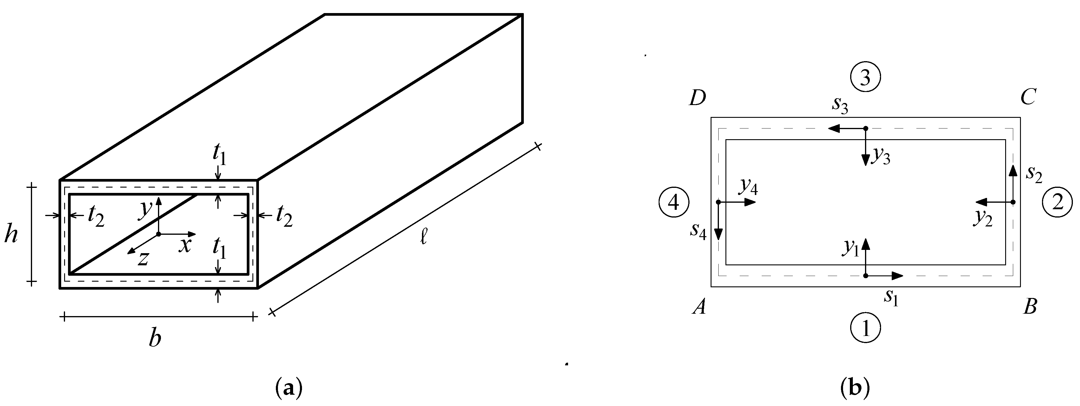
3. A Minimal GBT Model
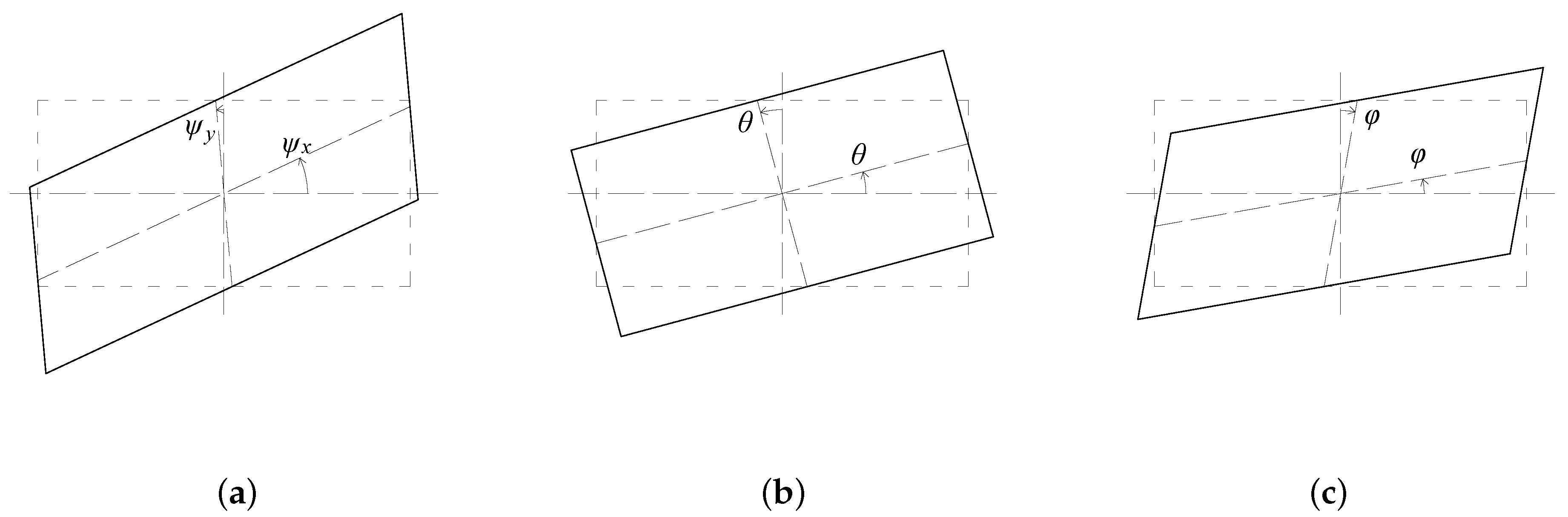
A rectangular, b × h , double-symmetric box-girder is considered (Figure 1). Its cross section is made of four thin elements: the bottom/upper flanges i = 1 , 3 , of thickness t 1 = t 3 , and the right/left webs i = 2 , 4 , of thickness t 2 = t 4 . A simple model is formulated, aimed at capturing the main mechanical behavior of the twist-distortional behavior. The task is accomplished by following the GBT approach, in which just two modes are considered: (i) the torsional mode, in which the cross section keeps its shape unaltered, and (ii) the distortional mode, in which the cross section is deformed. According to Equation (3), the local displacement field is expressed as follows:
u z , s v z , s w z , s = θ z U t s V t s W t s + φ z U d s V d s W d s
where the s-functions are the components of the two modes, to be properly chosen, and a = θ z , φ z T are the unknown amplitude functions, measuring the magnitude of twist θ and distortion φ .
To define the amplitudes, a general inextensional transformation of the box-girder is considered (by ignoring, at this stage, compatibility at corners), in which the x-axis rotates of an angle ψ x and the y-axis of an angle ψ y , both positive counterclockwise (Figure 2a). By decomposing the transformation in its skew-symmetric (Figure 2b) and symmetric (Figure 2c) parts, the twist θ and the distortion φ are uniquely determined as follows:
θ = 1 2 ψ x + ψ y , φ = 1 2 ψ x ψ y
together with their inverse ψ x = θ + φ , ψ y = θ φ .
To define the modes, a suitable in-plane field U s , V s is chosen, as illustrated ahead. From this, the warping component W s is derived by exploiting the internal constraint condition γ z s z , s t s = ϕ z , borrowed by the Bredt theory. Since, in a generic mode, γ z s = u , z + w , s = U s + W s a z , the constraint entails U s + W s t s = const = : Q . This equation can be integrated to furnish
W = 0 s U s d s + Q 0 s d s t s + C
where C is a further integration constant. The previous result is particularized to the two modes.

3.1. Torsional Mode

The in-plane displacement field is expressed as a rotation θ = 1 around the centroid, entailing (Figure 3a,b)
U t i = h 2 i = 1 , 3 b 2 i = 2 , 4 , V t i = s i i = 1 , 4
where s i i = 1 , , 4 are local abscissas with origins at the midpoint of each element i. The associated warping is evaluated by Equation (12), applied to each element, which leads to the following:
W t i = h 2 + Q t t i s i + C i i = 1 , 3 b 2 + Q t t i s i + C i i = 2 , 4
where C i are integration constants. By enforcing continuity at the four corners and the condition Γ W s t s d s = 0 (for equilibrium along z), the five unknown are determined as C i = 0 and Q t = b h t 1 t 2 b t 2 + h t 1 . Therefore,
W t i = 2 w t b s i i = 1 , 3 2 w t h s i i = 2 , 4
where w t : = b h 4 b t 2 h t 1 b t 2 + h t 1 is the modulus of warping at the corners (Figure 3c). This expression coincides with that in Equation (A1) of Appendix A, obtained by the Vlasov theory; therefore, W t i ω s . It should be noticed that the torsional warping vanishes when b h = t 1 t 2 .

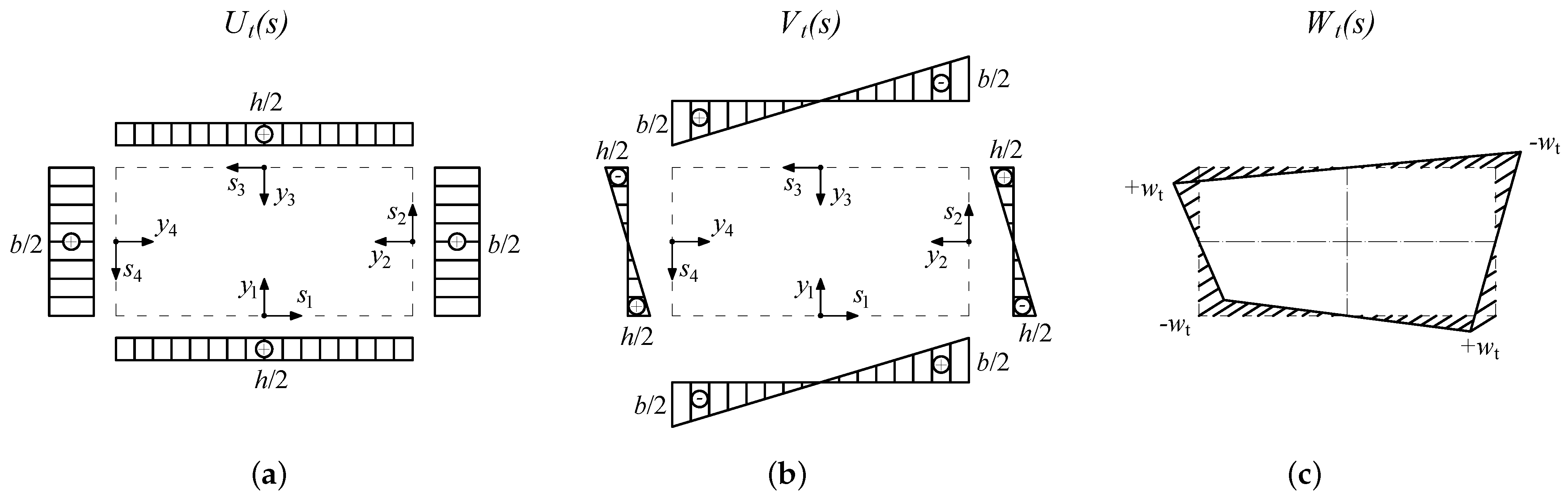
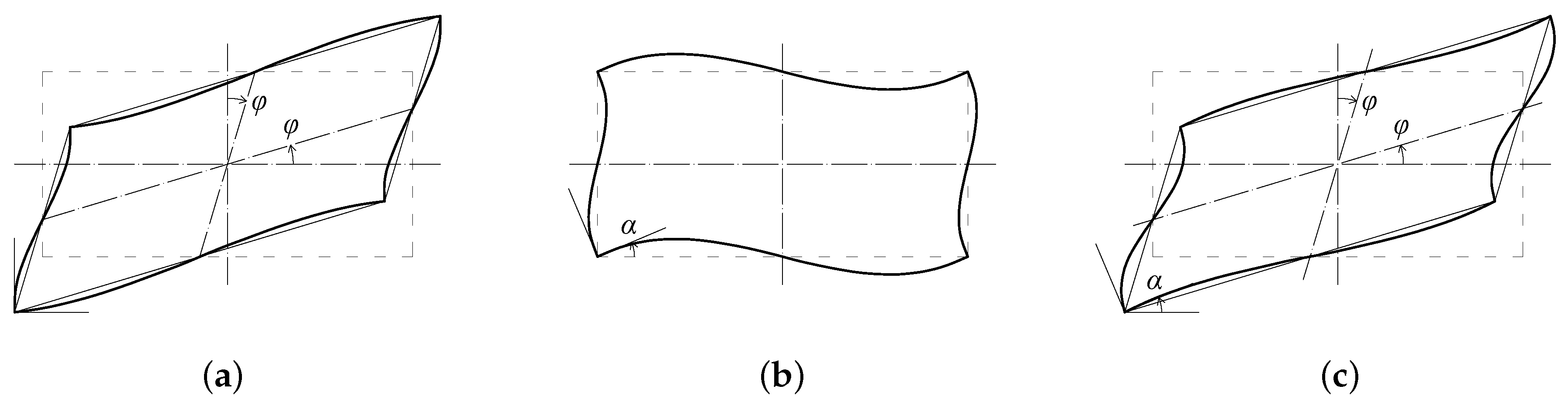
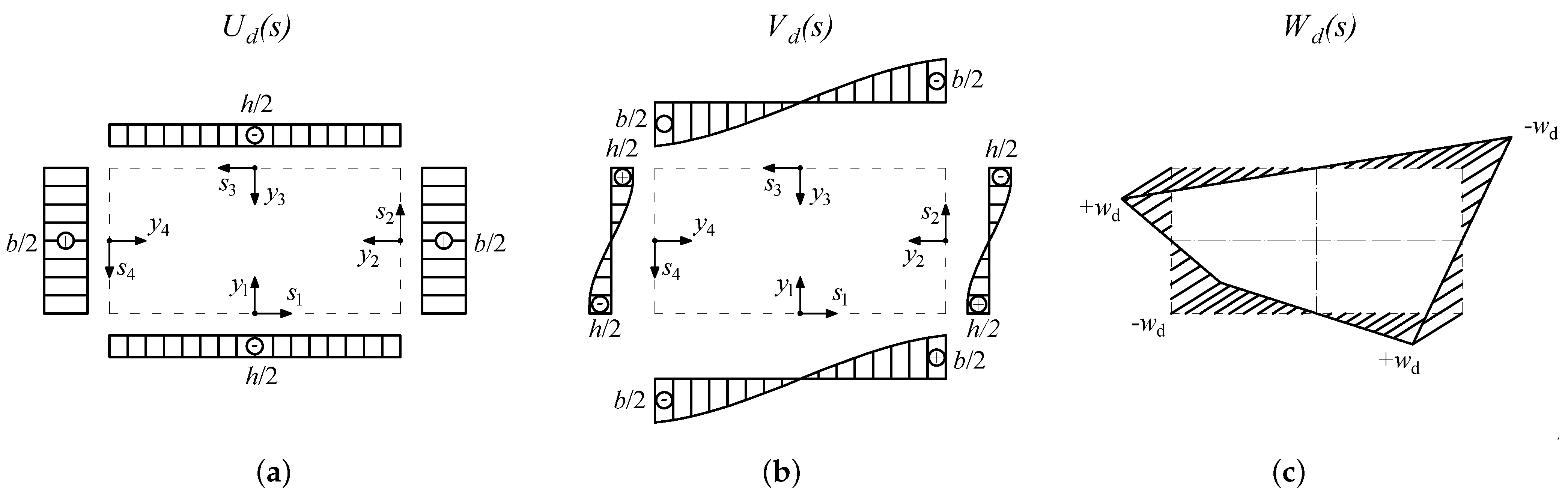
3.2. Distortional Mode

The in-plane displacement field is found as that experienced by a planar frame, undergoing displacements at joints, namely (i) prescribed translation of joints, caused by a distortion φ = 1 , with no rotations, (Figure 4a); (ii) unknown rotations of joints of equal amplitude α with no translations (Figure 4b). After having determined the moments at any of the the four joints, equilibrium is enforced, from which the unknown is evaluated as follows:
α : = b t 2 3 h t 1 3 b t 2 3 + h t 1 3
referred to below as the distortional joint rotation (which can be positive, nil, or negative according to the geometric parameters. After that, the transverse displacements are computed by integrating the elastic line equation under now-known translations and rotations at the ends (see Appendix B for details). The tangential displacements are instead immediately evaluated from the kinematics illustrated in Figure 4a. By summarizing (Figure 5a,b),
U d i = h 2 i = 1 , 3 b 2 i = 2 , 4 , V d i = 1 2 s i 3 + 4 s i 2 α 1 b 2 α i = 1 , 3 1 2 s i 3 + 4 s i 2 α + 1 h 2 α i = 2 , 4
to obtain the warping component, the procedure already described for the torsional mode is followed, leading to the following:
W d i = h 2 + Q d t i s i + C i i = 1 , 3 b 2 + Q d t i s i + C i i = 2 , 4
Due to the skew-symmetric nature of U d i , continuity at joints and the zero-average condition require C i = Q d = 0 . Therefore,
W d i = 2 w d b s i i = 1 , 3 2 w d h s i i = 2 , 4
where w d : = b h 4 is the modulus of the warping at joints (Figure 5c).
It is worth noticing that, differently from torsion, the distortional warping never vanishes. The two warping components are proportional (Figure 3c and Figure 5c), i.e., W t ( s ) = β W d ( s ) , with
β : = b t 2 h t 1 b t 2 + h t 1
defined as the warping ratio. The plot of β vs. the aspect ratio b h , for different thickness ratios t 1 t 2 , is represented in Figure 6. In the range examined, β spans the interval 1 , 1 , so that the two warpings (for unitary twist and distortion) are of the same order of magnitude, except close to a critical combination of the parameters, for which torsional warping is zero.

3.3. GBT Equations

By using the torsional mode (Equations (13) and (15)) and the distortional mode (Equations (17) and (19)), the 2 × 2 matrices (Equation (8) appearing in the GBT equations (Equation (7)) are evaluated, for which the components are as follows:
C α β e = E Γ t W α W β d s , C α β f = Γ D V α V β d s D α β f = ν Γ V α V β d s , D α β t = G 3 Γ t 3 V α V β d s D α β s = G Γ t ( W α + U α ) ( W β + U β ) d s B α β f = E 12 Γ t 3 V α V β d s , B α β d = E Γ t U α U β d s α , β = t , d
together with a = θ , φ T , p = c t , c d T , in which c α is the couples per unit length. A careful check of these matrices reveals the following:
  • since U t ( s ) and U d ( s ) are step-wise constant, U t = U d = 0 , and therefore B d = 0 (i.e., no in-plane dilatation occurs);
  • since V t s is step-wise linear and V d s quadratic, then B 11 f = B 12 f = B 21 f = 0 , so that only B 22 f 0 in matrix B f ;
  • since W t + U t = Q t 0 (torsional shear different from zero) and W d + U d = Q d = 0 (distortional shear zero), then D 12 s = D 21 s = D 22 s = 0 , so that only D 11 s 0 in matrix D s ; the implications on stresses of Q d = 0 will be discussed ahead.
Moreover, aimed at obtaining the simplest model, the Poisson ratio is taken as zero, so that D f = 0 . Concerning D t , it accounts for linear distribution of the tangential stresses in the thickness. When TWBs are considered, these terms are usually negligible with respect to the Bredt stresses; however, in the case of reinforced concrete box-girder bridges, where thicknesses are not so small, they can give significant contributions, as it will be shown by numerical simulations. Therefore, matrix D t is retained in the analysis.
As a result, the field GBT equations reduce to the following:
C 11 C 12 C 21 C 22 θ φ + D 11 D 12 D 21 D 22 θ φ + 0 0 0 B 22 f θ φ = c t c d
where C i j : = C i j e + C i j f and D i j : = D i j s + D i j t , together with the following boundary conditions:
δ θ δ φ T C 11 C 12 C 21 C 22 θ φ 0 = 0 0 δ θ δ φ T C 11 C 12 C 21 C 22 θ φ D 11 D 12 D 21 D 22 θ φ 0 = 0 0
The explicit expressions of the matrices appearing in Equation (22) are reported in Appendix C. It is worth noticing that, when the distortion φ is ignored and the flexure of plates is neglected with respect to the membrane strains (i.e., C 11 f 0 , D 11 t 0 ), the GBT equations reduce to Equation (2) of the Vlasov theory, with C 11 e = E I ω , D 11 s = G J . When torsion is ignored (together with C 22 f 0 , D 22 t 0 ) and distortion is artificially uncoupled, the GBT equations reduce to the classic equation of the beam on elastic soil, on which the BEF analogy is founded.

3.4. Stresses

Once the GBT equations are solved and the amplitudes θ z , φ z are evaluated, the active stresses can be computed by coming back to Equation (5). Reactive stresses, instead, must be determined from equilibrium. By separating the effects of the two modes, the following results are drawn (with the Poisson ratio taken zero). Moreover, from now on, τ : = τ z s is used to simplify the notation.
In the torsional mode, the active stresses are as follows:
σ s m ( z , s ) = 0 σ z m ( z , s ) = E 2 h β s i θ ( z ) i = 1 , 3 E 2 b β s i θ ( z ) i = 2 , 4 τ m ( z , s ) = G b h t 2 h t 1 + b t 2 θ ( z ) i = 1 , 3 G b h t 1 h t 1 + b t 2 θ ( z ) i = 2 , 4 σ s f ( z , s ) = 0 σ z f ( z , s ) = E y i s i θ ( z ) i = 1 , 4 τ f ( z , s ) = 2 G y i θ ( z ) i = 1 , 4
and the reactive stresses (see the Appendix A) are as follows:
τ m r z , s = E θ z h h t 1 b t 2 3 h b 2 4 s i 2 t 1 + b b 2 + 2 h 2 6 s i 2 t 2 48 h t 1 + b t 2 2 i = 1 , 3 E θ z b h t 1 b t 2 h 2 b 2 + h 2 12 s i 2 t 1 + 3 b h 2 4 s i 2 t 2 48 h t 1 + b t 2 2 i = 2 , 4
The normal stresses σ z m ( z , s ) coincide with those predicted by the Vlasov theory (see Equation (A3) in Appendix A), while the tangential stresses τ m ( z , s ) coincide with those of the Bredt theory (see Equation (A4) in Appendix A). The reactive tangential stresses τ m r cannot be captured by the constitutive law of the GBT model (which is based on the same Vlasov kinematic constraint on the flow).
The relevant stress-fields are qualitatively depicted in Figure 7 at a generic cross-section; there, the index max denotes evaluation at the top/bottom face of the plates (i.e., at y i = ± t i 2 ). The diagrams repeat themselves at any abscissas z, being altered by a factor proportional to θ z , θ ( z ) , θ ( z ) , as stated by Equations (24) and (25). The membrane normal stresses σ z m (Figure 7a) are caused by nonuniform warping; they are proportional to W t s (Equation (15)) and vary on z as θ z . The flexural normal stresses σ z f (maximum value in Figure 7b) are caused by the flexure of plates in the longitudinal direction; they are proportional to V t s (Equation (13)) and depend on z via θ z . The membrane active tangential stresses τ m (Figure 7c) are consistent with the Bredt behavior of the box; they are step-wise constant on the cross section and vary with θ z . The reactive component τ m r (Figure 7d) must be added to them; they are step-wise parabolic on the cross section and vary with θ z . The flexural tangential stresses τ f (maximum value in Figure 7e) are related to the torsion of the plates; being proportional to V t s , they are step-wise constant on the cross section and vary with θ z .
In the distortional mode, the active stresses are as follows:
σ s m ( s , z ) = 0 σ z m ( s , z ) = E 2 h s i φ ( z ) i = 1 , 3 E 2 b s i φ ( z ) i = 2 , 4 τ m ( s , z ) = 0 σ s f ( s , z ) = E y i 12 α 1 b 2 s i φ ( z ) i = 1 , 3 E y i 12 α + 1 h 2 s i φ ( z ) i = 2 , 4 σ z f ( s , z ) = E 2 y i s i 3 + 4 α 1 s i 2 b 2 α φ ( z ) i = 1 , 3 E 2 y i s i 3 + 4 α + 1 s i 2 h 2 α φ ( z ) i = 2 , 4 τ f ( s , z ) = G y i b 2 b 2 α 3 12 α 1 s i 2 φ ( z ) i = 1 , 3 G y i h 2 h 2 α + 3 12 s i 2 α + 1 φ ( z ) i = 2 , 4
with α defined in Equation (16). For the torsional mode as well, the membrane reactive tangential stresses must be determined from equilibrium, leading to the following (see the Appendix D):
τ m r z , s = b h 48 2 b t 1 + h t 2 t 1 1 4 h s i 2 E φ ( z ) i = 1 , 3 b h 48 b t 1 + 2 h t 2 t 2 + 1 4 b s i 2 E φ ( z ) i = 2 , 4
The relevant stress-fields (with max denoting evaluation at y i = ± t i 2 ) are qualitatively depicted in Figure 8. The diagrams repeat themselves at any abscissas z, being altered by a factor proportional to φ ( z ) , φ ( z ) , φ ( z ) , as stated by Equations (26) and (27). The membrane normal stresses σ z m (Figure 8a) are caused by nonuniform warping; they are proportional to W d s (Equation (19)) and vary on z as φ z . The flexural normal stresses σ z f (maximum value in Figure 8b) are due to the longitudinal flexure of plates; they, being proportional to V d s (Equation (17)), are cubic on the cross section and depend on z via φ z . The transverse flexural normal stresses σ s f (maximum value in Figure 8c) are generated by the flexure of the plates in the transverse direction; being proportional to V d s , they are step-wise linear on the cross section and are modulated by φ z . The membrane reactive tangential stresses τ m r (Figure 8d) are step-wise parabolic and proportional to φ z . The flexural tangential stresses τ f (maximum value in Figure 8e) are related to the torsion of the plates; they depend on V d s , are step-wise parabolic on the cross section, and are modulated by φ z .
It is worth noticing that, according to the model presented here, the distortional tangential stresses are purely reactive, since no shear strains occur in the distortional mode; in contrast, longitudinal normal stresses are of the active type, directly related to distortional warping. The model, therefore, is different from that adopted in Reference [8], where due to the assumed step-wise constant shear with no warping, the tangential stress is active while the normal stress is reactive. As an advantage of the method followed here, the continuity of the flow of tangential stresses is assured at the joints, a condition that cannot be satisfied in the alternative approach.

4. Algorithmic Aspects

Aimed at further simplifying the reduced GBT equations (Equation (22)), an analysis of the relative magnitude of different terms is carried out. Moreover, qualitative information on the relative importance between distortion and twist are sought. Then, some methods of solution are discussed.

4.1. Order of Magnitude of the Coefficients and Unknowns

The possibility to neglect some terms in GBT equations depending on the geometric quantities involved is detected.

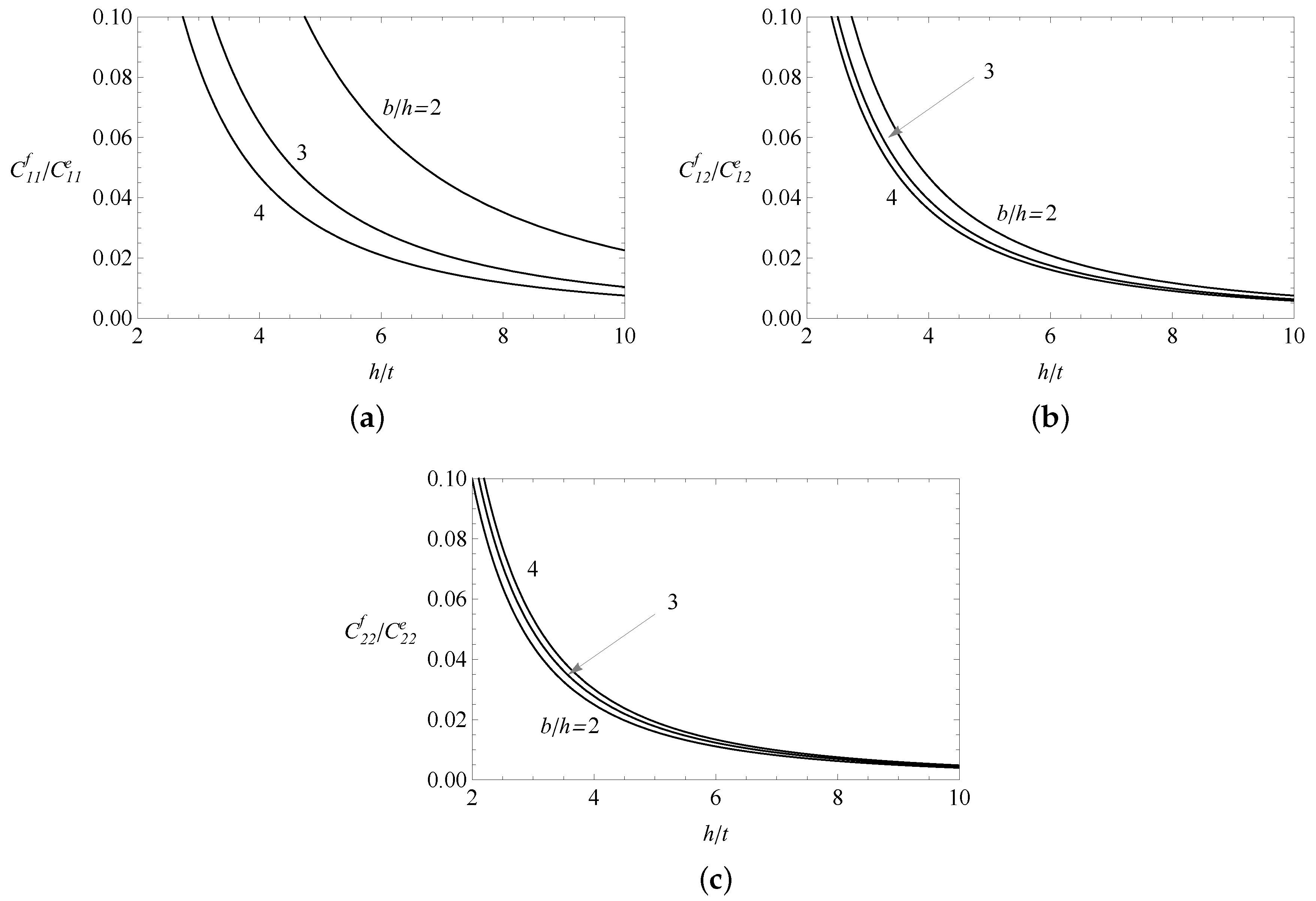
4.1.1. Flexural vs. Extensional Higher-Order Derivatives

First, the coefficients of the higher-order derivatives, C i j = C i j e + C i j f , are considered. In them, it is expected that the C i j f s, which account for longitudinal flexure of the thin plates, are much smaller than the C i j e s, which account for extension of the longitudinal fibers induced by nonuniform warping (at least in the distortional mode, where warping never disappears). To investigate this aspect, the ratios C i j e / C i j f are plotted in Figure 9 vs. the h t ratio for different b h ratios and for a fixed t 2 t 1 . It is seen that, for realistic values of h t , e.g., ranging between 5 and 10, the flexural coefficients are, as expected, a small fraction (few percents) of the extensional ones. It is concluded that the C i j f are generally negligible, especially for large h t . An exception, of course, occurs when C 11 e = C 12 e = 0 .

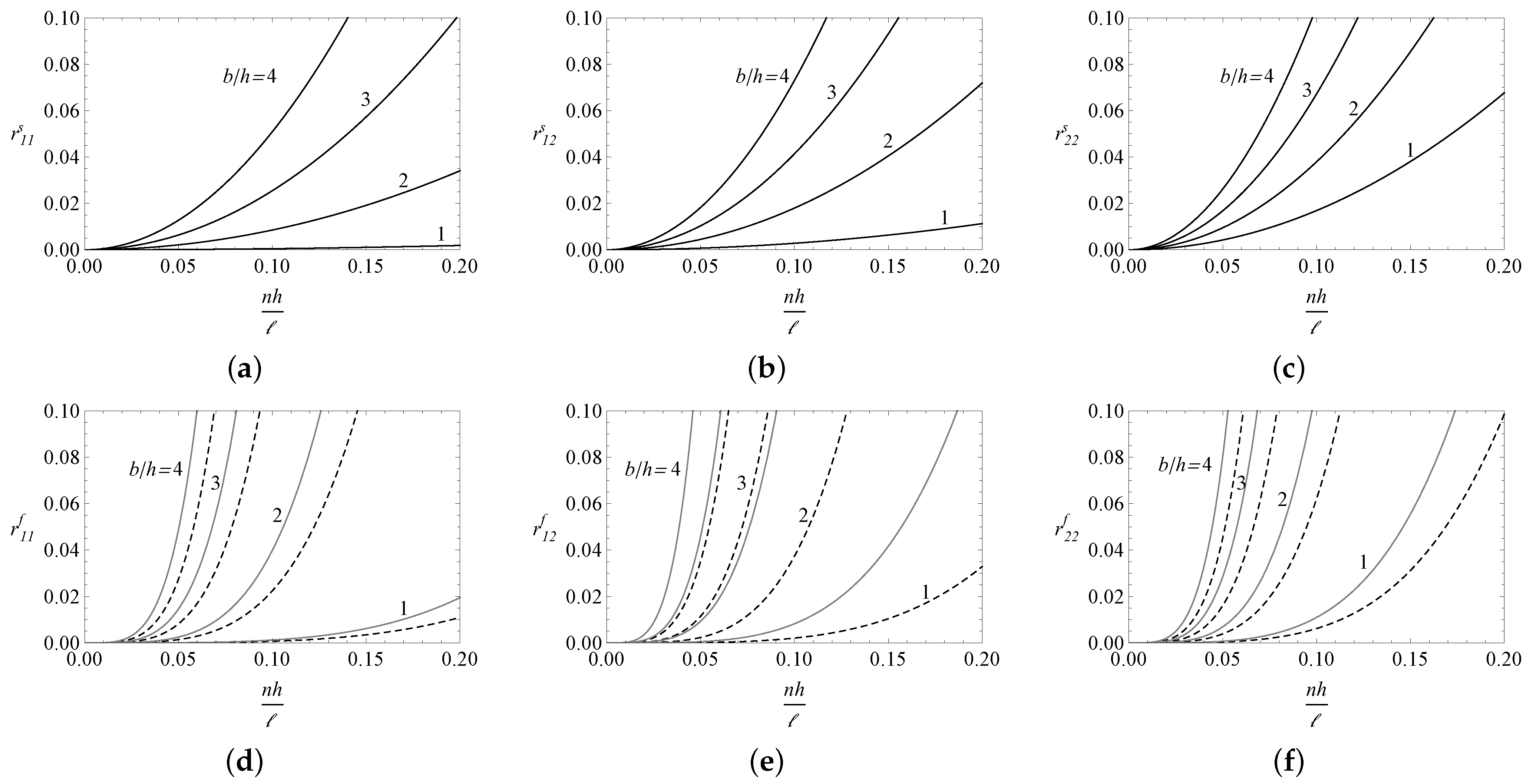
4.1.2. Extensional vs. Shear Torsional Effects

A second, and more important, topic concerns coupling existing between the GBT equations. They are a set of two fourth-order differential equations, where coupling is mainly due to higher-order terms (the larger ones being produced by warping, as seen before). It is interesting to investigate if, and under which conditions, such a coupling can be neglected. To this end, the box-girder is assumed to be loaded by sinusoidal loads p = c t ^ , c ^ d T sin n π z , which trigger sinusoidal deflections a = θ ^ , φ ^ T sin n π z . The amplitudes must satisfy the following algebraic equations:
C 11 e C 12 e C 21 e C 22 e n π 4 + D 11 s 0 0 0 n π 2 + 0 0 0 B 22 f θ ^ φ ^ = c ^ 1 1
where c t ^ = c ^ d = c ^ has been taken and C i j f is neglected together with D i j t (small thickness). The task is understanding if the C i j e s bring a significant contribution to the equilibrium when, e.g., they are compared to D 11 s = G J or B 22 f . Referring to a rectangular box-girder with uniform thickness t 1 = t 2 = : t , the nondimensional ratios r i j s : = C i j e D 11 s n π 2 and r i j f : = C i j e B 22 f n π 4 among the coefficients are plotted in Figure 10 vs. the squatness ratio n h for different b h . It is seen that the r i j s are less than 0.1 if n h < 0.2 (e.g., n < 4 if = 20   h ). Moreover, r i j s is much smaller as b h decreases, tending towards a square shape. Concerning r i j f , similar consideration hold.
The investigation therefore leads to the following conclusions:
  • Warping, as expected, plays a minor but not negligible role in torsion of closed TWB. In particular, it is fundamental in describing boundary layers close the constraints (or lumped forces), which, in a Fourier perspective, call for higher-order harmonics (n large), which make the fourth-order derivatives comparable with second- or zero-order derivatives.
  • Due to the small but not negligible coupling terms due to warping, the torsion–distortion mechanical problem cannot, in principle, be uncoupled, as already observed, e.g., in Reference [8]. A measure of the error made in splitting the problem will be discussed with reference to the numerical results.

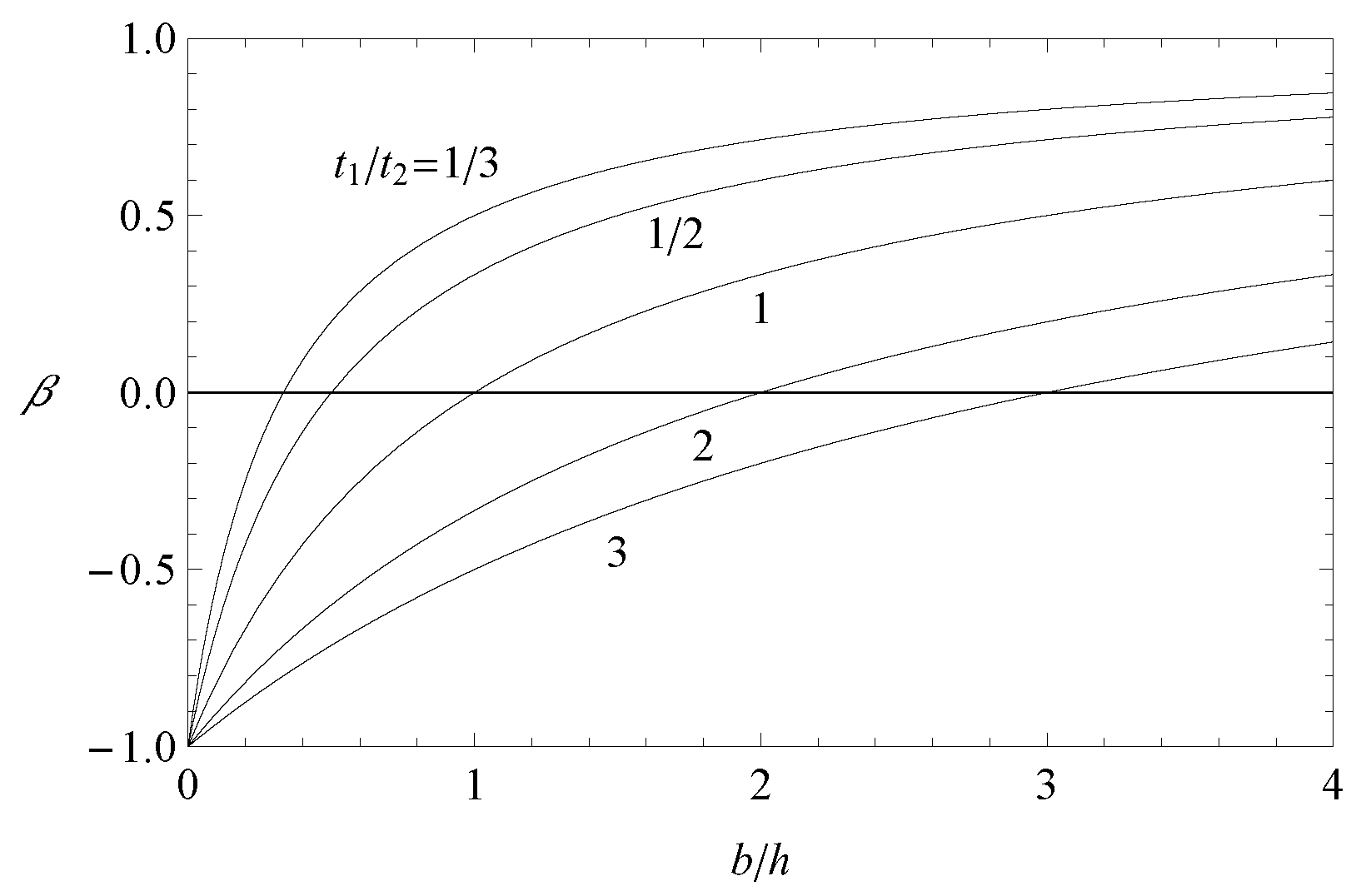
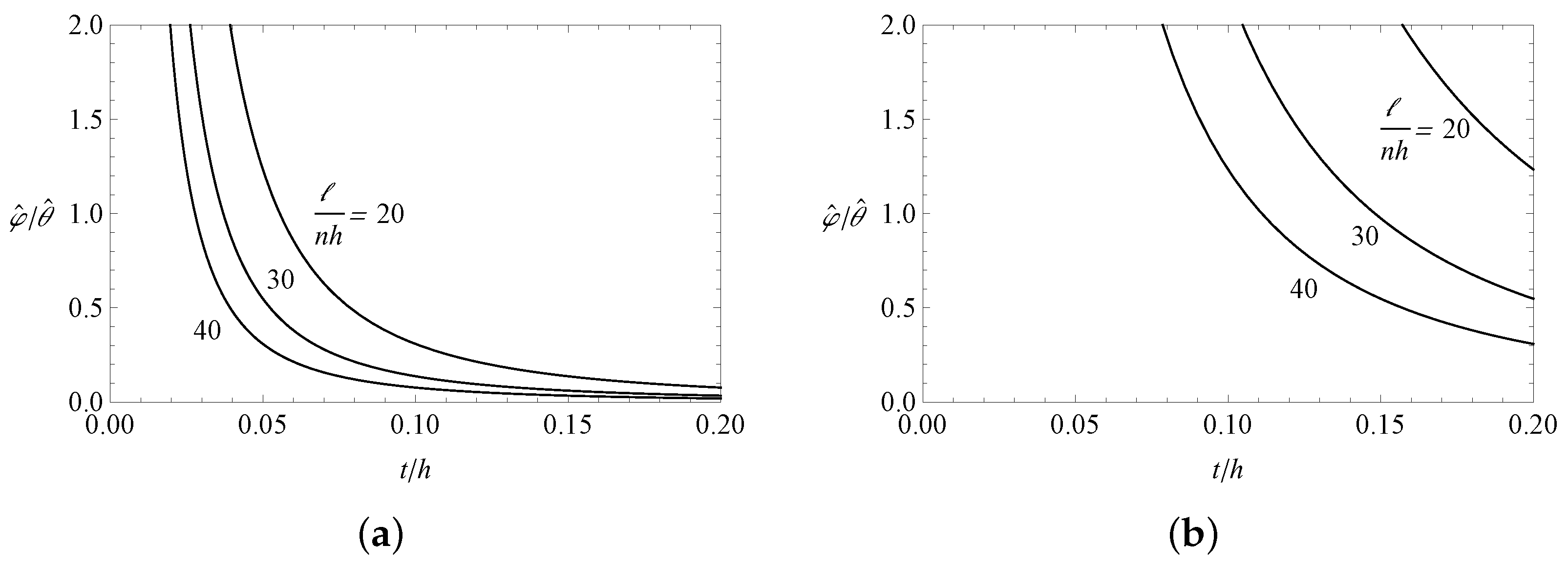
4.1.3. Distortional vs. Twist Amplitude

If, in a first attempt, the warping effects are completely neglected (i.e., C i j e = 0 is taken) together with the torsional curvatures (i.e., D i j t = 0 ), the two Equation (28) uncouple. Their solution gives a rough estimation of the relative importance of the distortion on twist, namely
φ ^ θ ^ = π 2 D 11 s B 22 f
This ratio is plotted in Figure 11 vs. t h for squared (Figure 11a) and rectangular (Figure 11b) boxed cross sections having uniform thickness t 1 = t 2 = : t and for different slenderness ratios n h . It appears that distortion is of the same order as twist or even larger:
  • for a fixed slenderness ratio n h , distortion is larger for smaller thicknesses;
  • for a fixed thickness ratio t h , distortion is larger for shorter lengths.
The results corroborate and quantify the common idea that the girder behaves as a beam (i.e., with no distortion) when it is long and its cross section is thick.

4.2. Solution Methods

The exact integration of the complete GBT equations, although not difficult in principle, is quite laborious. As a matter of fact, when boundary layers exist, even exact closed-form solution are not well-conditioned and numerical problems arise. To confine the analysis to a minimum level, two approaches are proposed here: (a) an exact Fourier analysis, holding for simply supported box-girder with free warping at the ends; (b) an exact closed-form solution for simplified equations, heuristically obtained by neglecting coupling.

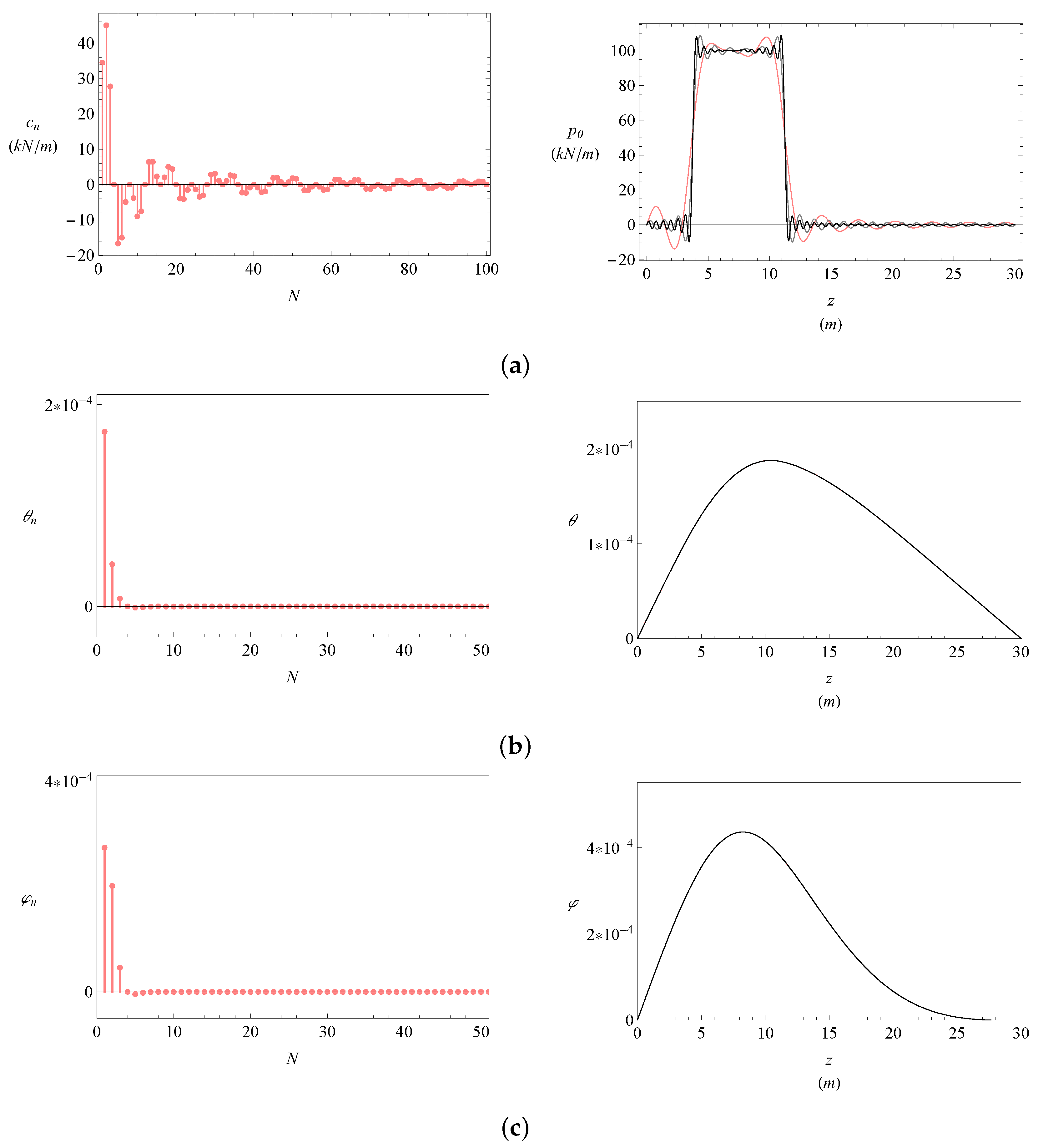
4.2.1. Fourier Analysis

The modal loads c t , c d are expanded in Fourier sinus series as c α = n = 1 N c α n sin n π z with α = t , d . Accordingly, generalized displacements are expanded as well as
θ φ = n = 1 N θ n φ n sin n π z
with θ n , φ n unknowns. By substituting the series in the GBT equations (Equation (22)) and by separating the harmonics, we obtain the following (apex omitted on B 22 ):
D 11 π 2 n 2 2 + C 11 π 4 n 4 4 D 12 π 2 n 2 2 + C 12 π 4 n 4 4 D 21 π 2 n 2 2 + C 21 π 4 n 4 4 B 22 + D 22 π 2 n 2 2 + C 22 π 4 n 4 4 θ n φ n = c t n c d n
From these equations, the unknowns are evaluated.

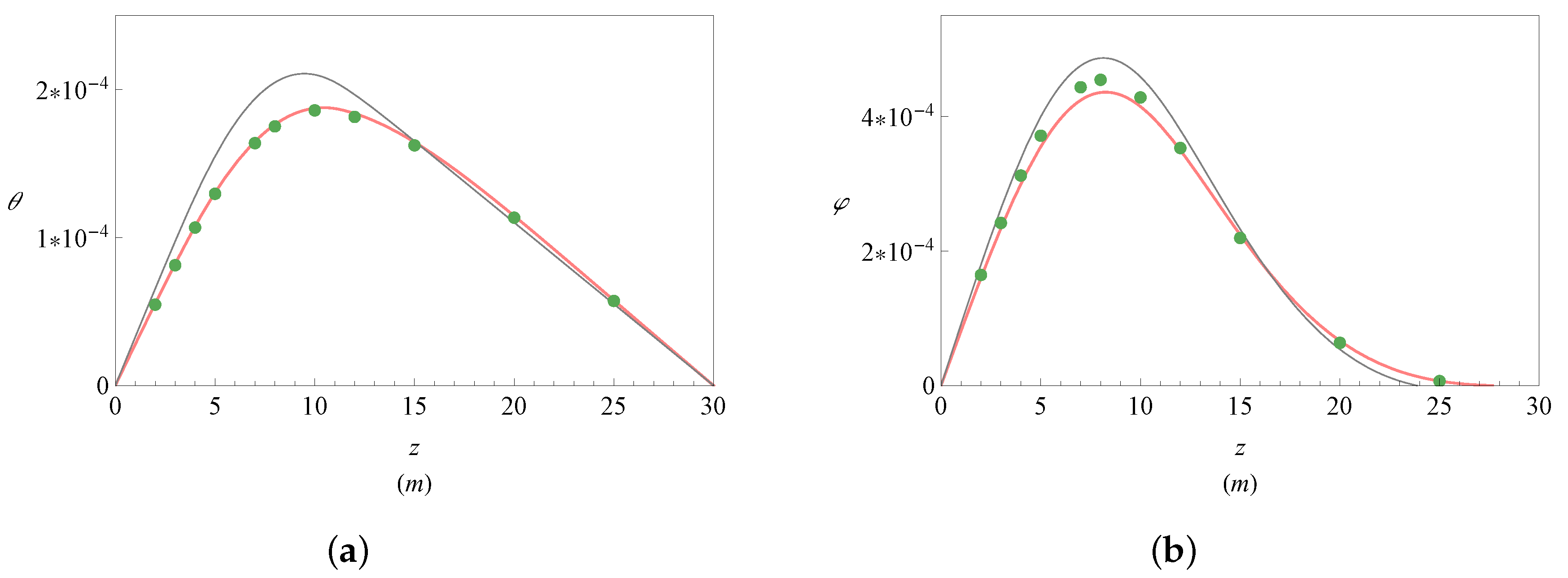
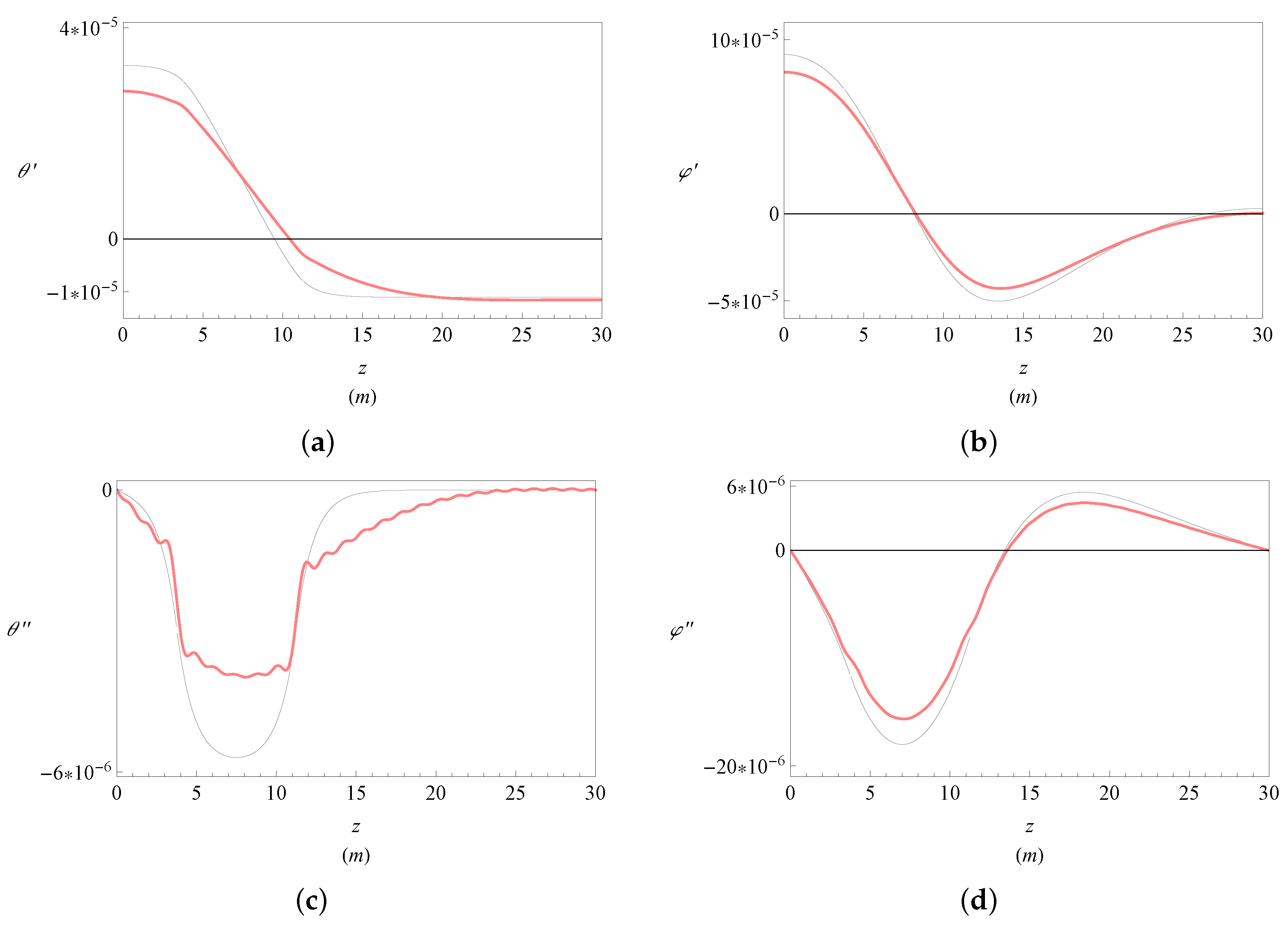
4.2.2. A Simplified Approach: The Uncoupled Equations

A heuristic approach is attempted here, consistent with the literature, in which all out-of-diagonal terms are (arbitrarily) neglected. In this case, the differential equations and boundary conditions read as follows:
E I ω θ G J θ = p t θ 0   = θ 0   = θ   = θ = 0
together with
C 22 φ + B 22 φ = p d φ 0   = φ 0   = φ   = φ = 0
The first equation coincides with Equation (2) of the Vlasov theory, while the second one is the classic equation of a beam on Winkler soil. It should be noticed that, according to this simplified approach, distortional stresses simply add themselves to Vlasov stresses without any feedback effect.
Integration usually calls for dividing the 0 , interval in subintervals in which the loads are continuous; in the generic subinterval i, the general solution reads as follows:
θ z i   = c 1 i e λ z i l i + c 2 i e λ z i + c 3 i z i + c 4 i + θ ¯ i z i φ z i   = e μ z c 1 i sin μ z   +   c 2 i cos μ z   +   e μ z c 3 i sin μ z   +   c 4 i cos μ z   +   φ ¯ i z i
where l i is the lengths of the subintervals, z i is the local abscissas spanning them, with the origin at the left end; and c k i is an arbitrary constant. Moreover, θ ¯ i z i , φ ¯ i z i are particular solutions. Finally,
λ : = G J E I ω , μ : = B 22 4 C 22 4
are wave numbers.
The arbitrary constants c j i appearing in each problem are determined by enforcing two boundary conditions at each z = 0 , end and four conditions at each of the internal boundaries, as supplied by Equation (23). If no lumped couples are present, these read as follows:
  • for the twist problem, (i) continuity of θ , (ii) continuity of θ , (iii) equilibrium of forces dual of δ θ (entailing continuity of the bimoment B = E I ω θ ), and (iv) equilibrium of forces dual of δ θ (entailing continuity of the total torsional moment M ¯ t = G J θ E I ω θ );
  • for the distortional problem, (i) continuity of φ , (ii) continuity of φ , (iii) equilibrium of forces dual of δ φ (entailing continuity of φ ), and (iv) equilibrium of forces dual of δ φ (entailing continuity of φ ).
By numerically solving two sets of linear algebraic problems, the arbitrary constants are evaluated and the solution (Equation (34)) is analytically obtained in step-wise form.

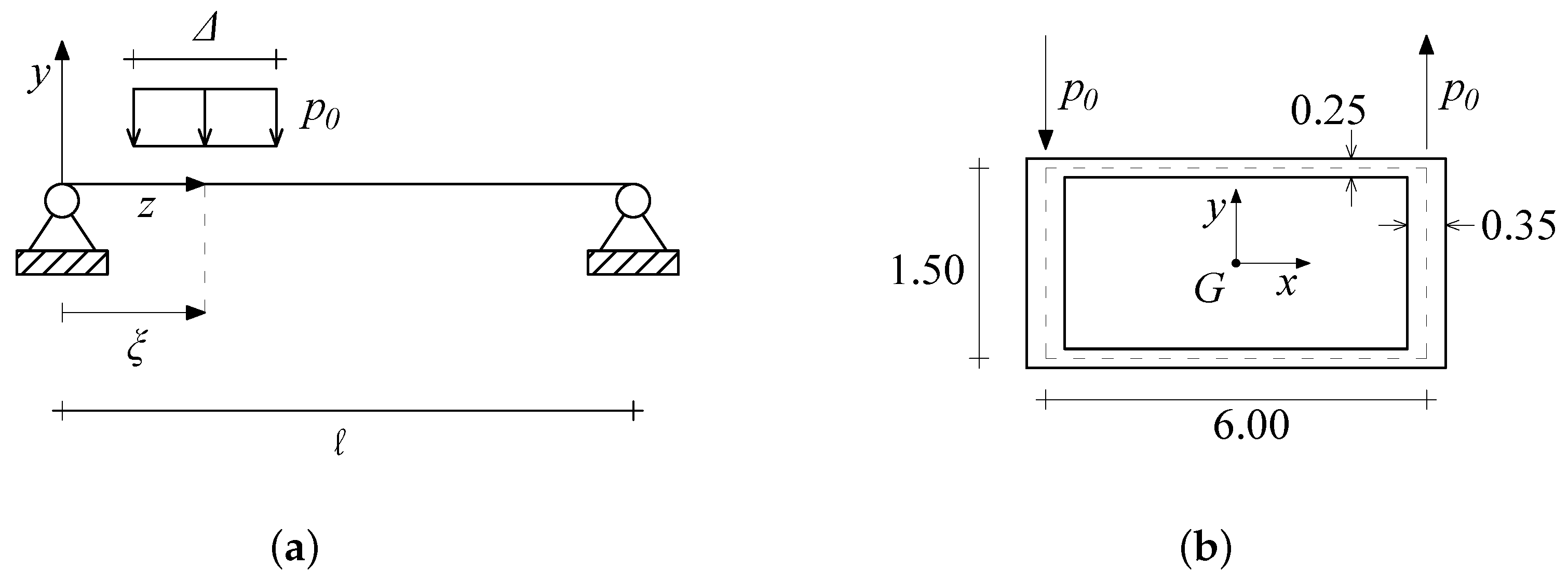
5. Numerical Results

A case study is considered, consisting of a reinforced concrete, rectangular box-girder bridge, taken from the literature [3]. The box-girder has the following geometric characteristics: length = 30   m , width b = 6   m , height h = 1.5   m , flange thickness t 1 = 0.25   m , web thickness t 2 = 0.35   m ; elastic moduli E = 35,654 × 10 3   kN / m 2 ,and G = E / 2 . The GBT constants consequently assume the values in Table 1. Moreover, the joint distortional rotation is α = 0.83 and the warping ratio β = 0.70 .
The girder is assumed to be simply supported at the end, where it is free to warp. It is loaded at the two webs by equal and opposite forces P = ± 750   kN , uniformly distributed on a length Δ = 4 , as p 0 : = ± P Δ = 100   kN / m , and centered at the abscissa: ξ = 4 (Figure 12). The relevant modal loads c t z , c d z are evaluated by Equation (9), as the virtual work spent at the abscissa z by the external forces in the displacements caused by θ = 1 and φ = 1 , respectively. Since, at the application points of the loads (i.e., at the corners C , D of the box, see Figure 1), it is V = ± b 2 in both modes, it follows that
c α x = p 0 b z ξ Δ 2 , ξ + Δ 2 0 z ξ Δ 2 , ξ + Δ 2 α = t , d
The elastic problem was tackled in different ways: (a) by solving the GBT Equation (22) (with no terms neglected) via Fourier series; (b) by exactly integrating the differential Equations (32) and (33) after having neglected the coupling terms; and (c) via a FEM analysis. The latter was carried out by using a commercial software by implementing a model made of 40 × 60 = 2400 shell elements (along the directrix and the axis, respectively) for an overall number of 2440 degrees of freedom. The results were then compared.

5.1. Deflection Analysis

First, Fourier analysis was carried out for the GBT equations. By expanding the modal loads in sinus Fourier series, the coefficients c t n = c d n = : c n were found, as reported in Figure 13a, together with the truncated series with N = 20 , 50 , 100 terms. The Fourier spectra for deflections, as furnished by Equation (31), together with the reconstructed series (for N = 50 , value used from now on) are represented in Figure 13b,c. As a general comment, distortion of the box girder is remarkable, larger than twist, and it propagates to a large distance from the loaded region.
The simplified method was successively applied by uncoupling the GBT equations. The integration domain was broken in three subintervals, i.e., I 1 : = 0 , ξ Δ 2 ,   I 2 : = ξ Δ 2 , ξ + Δ 2 ,   I 3 : = ξ + Δ 2 , , and the general solution (Equation (34)) was written in each of them. There, θ ¯ i z i = φ i ¯ z i = 0   i = 1 , 3 and θ ¯ 2 z 2 = b p 0 2 G J z 2 2 ,   φ ¯ 2 z 2 = b p 0 B 22 are the particular solutions. The twelve arbitrary constants c k i appearing in each problem were determined by enforcing two boundary conditions at each z = 0 , end and four conditions at each of the internal boundaries, as discussed before. The responses θ z , φ z thus obtained, Equation (34), are plotted in Figure 14 and compared with those of the complete Fourier analysis. Here, the exact numerical results, as provided by the FEM analysis are also reported. It appears that FEM and Fourier analysis are in excellent agreement, in spite of the stronger simplifications introduced in the analytical model. The simplified analysis also supplies satisfactory results (maximum error of about +11% on twist and about +10% on distortion), especially far from the loads. Differences with the exact results put into light the contribution of coupling, which should not be ignored, if more accurate results are desired. It is concluded that the error provided by the simplified approach is reasonable and that, at least in this case study, this method is conservative since it magnifies the deflection (in agreement with the conclusions of Reference [6]).
The first, second, and third derivatives of both θ z and φ z amplitudes, needed for stresses evaluation according to Equations (24)–(27), were then computed. In Figure 15, the Fourier (coupled) solution is compared with that of the simplified (uncoupled) method (comparison with FEM being not straightforward). It appears that, although small spurious oscillations persist with N = 50 , the Fourier solution is quite smooth. Concerning the third derivatives θ , φ , two peaks are noticed at the end-points of the loaded interval, denoting the occurrence of a strongly varying complementary torsional moment and its correspondent distortional quantity, which are almost zero anywhere else. The simplified method gives a good approximation of all the derivatives, except a large error on the second derivative of θ z , magnified at the loaded region, consistently with what is noticed in Figure 14.

5.1.1. Stress Analysis in Pure Torsion

A stress analysis was carried out by referring to the Fourier solution with N = 50 terms. The stresses were evaluated by referring to the uncracked cross section. In order to separate the causes of discrepancies between analytical and FEM analyses, the pure torsion case θ 0 ,   φ 0 was considered first, for which the Vlasov beam model is usually assumed to be accurate. Thus, the stresses provided by the analytical model via Equations (24) and (25) were compared with those furnished by a FEM model, in which indeformability of the cross section was enforced via “body constraints”, simulating thin diaphrams at any cross sections of the mesh. It should be remembered, that the analytical model proposed here reproduces the Vlasov model by further encopassing for variation in the stresses within the thickness.
The pattern of stresses on a tipical cross section was examined first. Figure 16 reports, by continuous/dashed lines, the analytical longitudinal normal stresses σ z , m a x m + f : = σ z m + σ z , m a x f and the tangential stresses τ m a x m + f : = τ m + τ m a x f evaluated at the middle abscissa of the load ( z = 7.5   m ) and at bottom/top edges of the cross section. The bullets represent numerical FEM results. It appears that the “enriched Vlasov model” captures very well the state of stress sufficiently far from the corners of the cross section. Close to them, indeed, and probably exhalted from the abrupt change in thickness, the tangential stresses violate the Bredt law; this occurrence, in turn, entails a local disturbance on the longitudinal stresses for equilibrium reasons. The maximum differences between analytical and numerical results are of the order of 10–15%.
The dependence of the stresses on the longitudinal abscissa was then investigated. Figure 17 shows how the normal stresses at the corners and the tangential stresses at the half side s i = 0 depend on z. It appears that the differences between the analytical and numerical models disappear at large distance from the load, thus confirming the local nature of the disturbance.
Concerning the tangential reactive stresses, which are related to the complementary torsional moment, they are negligibly small at z = 7.5   m (not shown here). However, as Figure 18 shows, they are significant at z = 11.25   m (i.e., where the load has a discontinuity point) according to the diagram of θ z in Figure 15e.

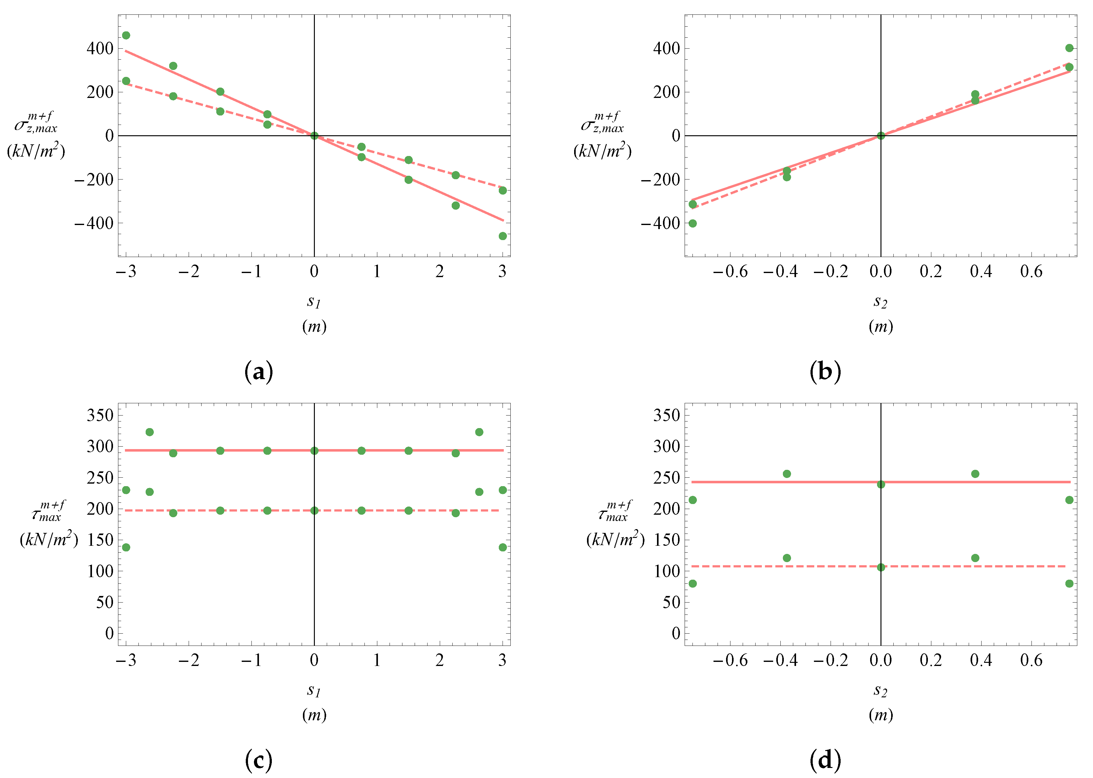
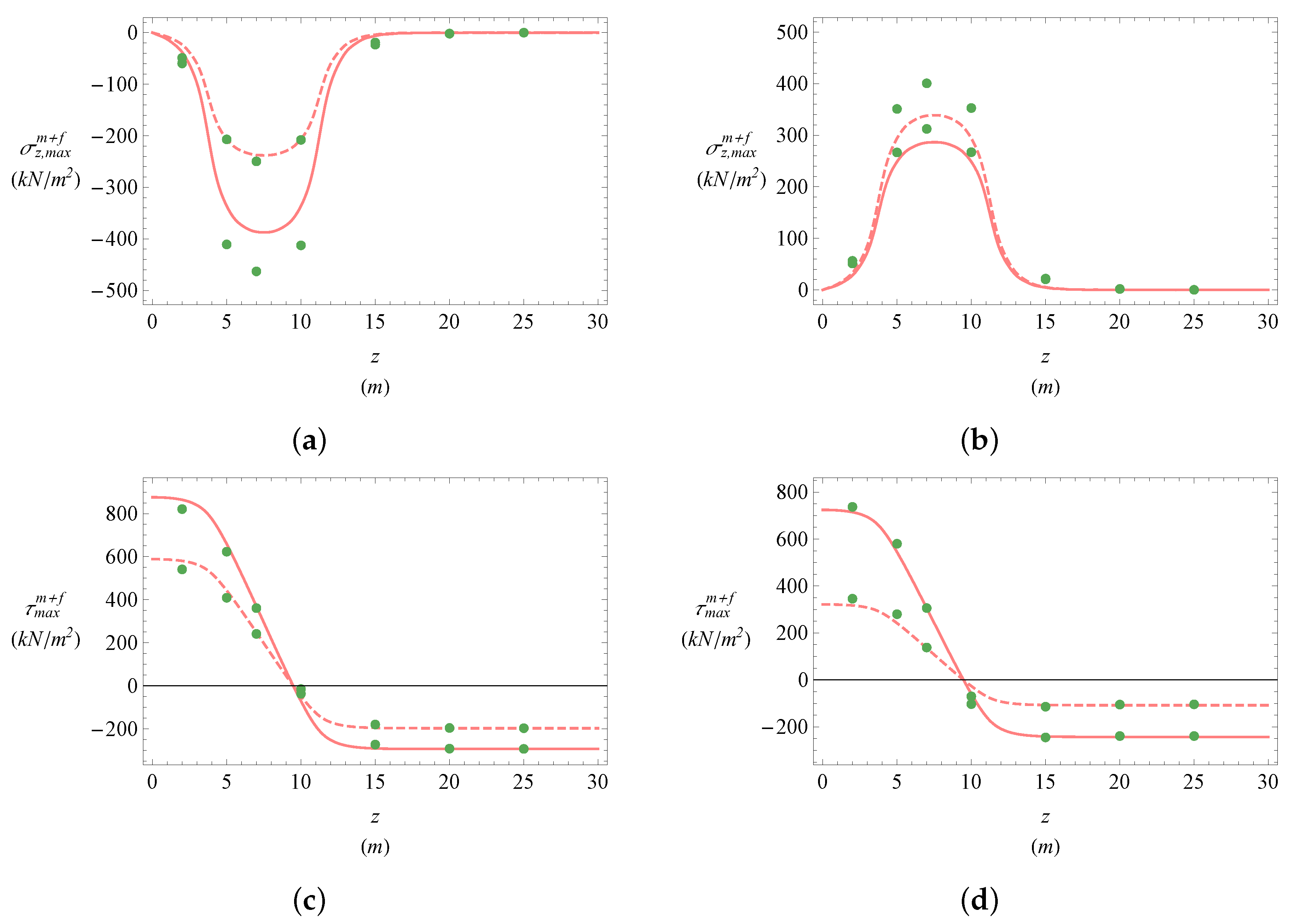
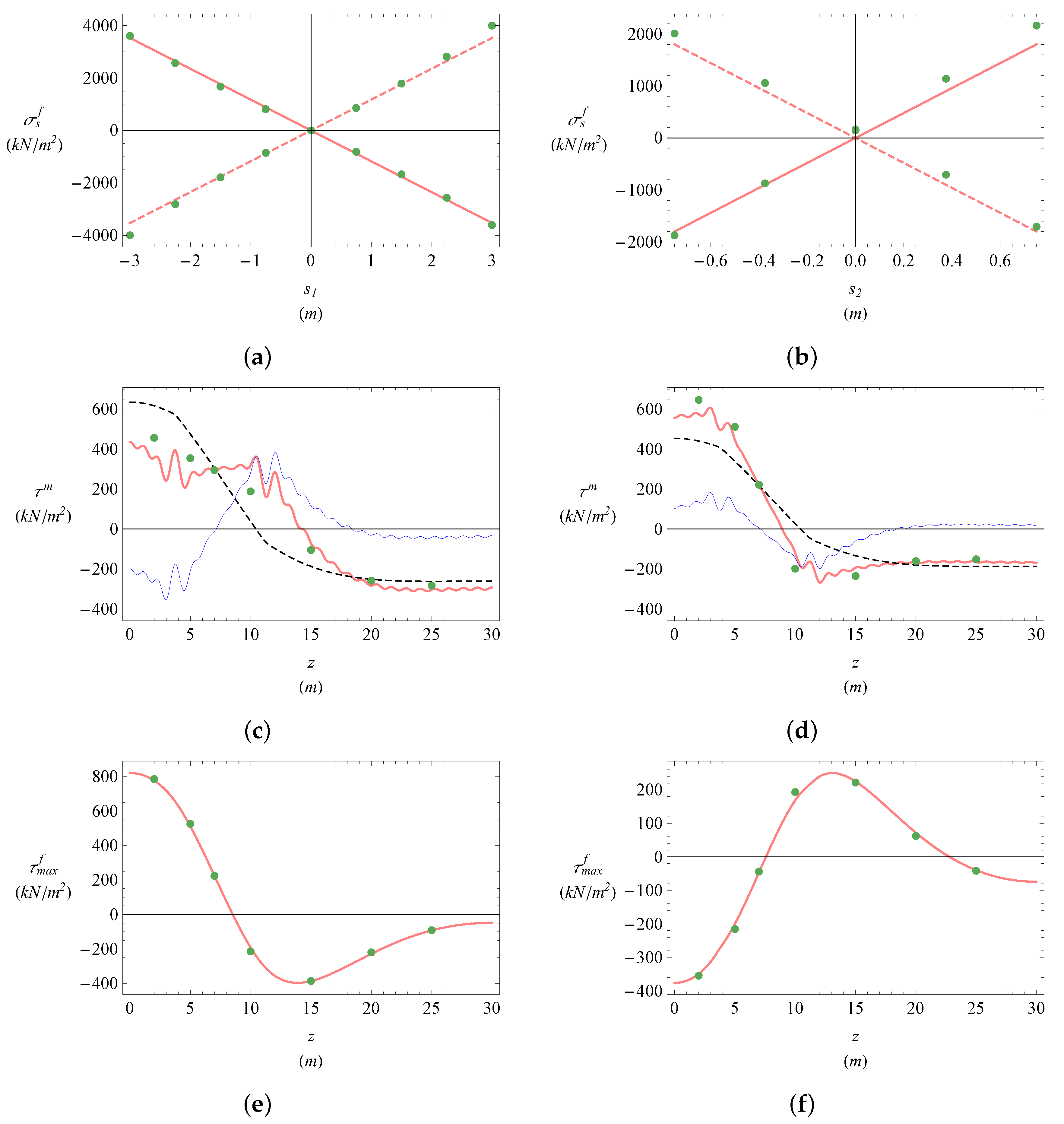
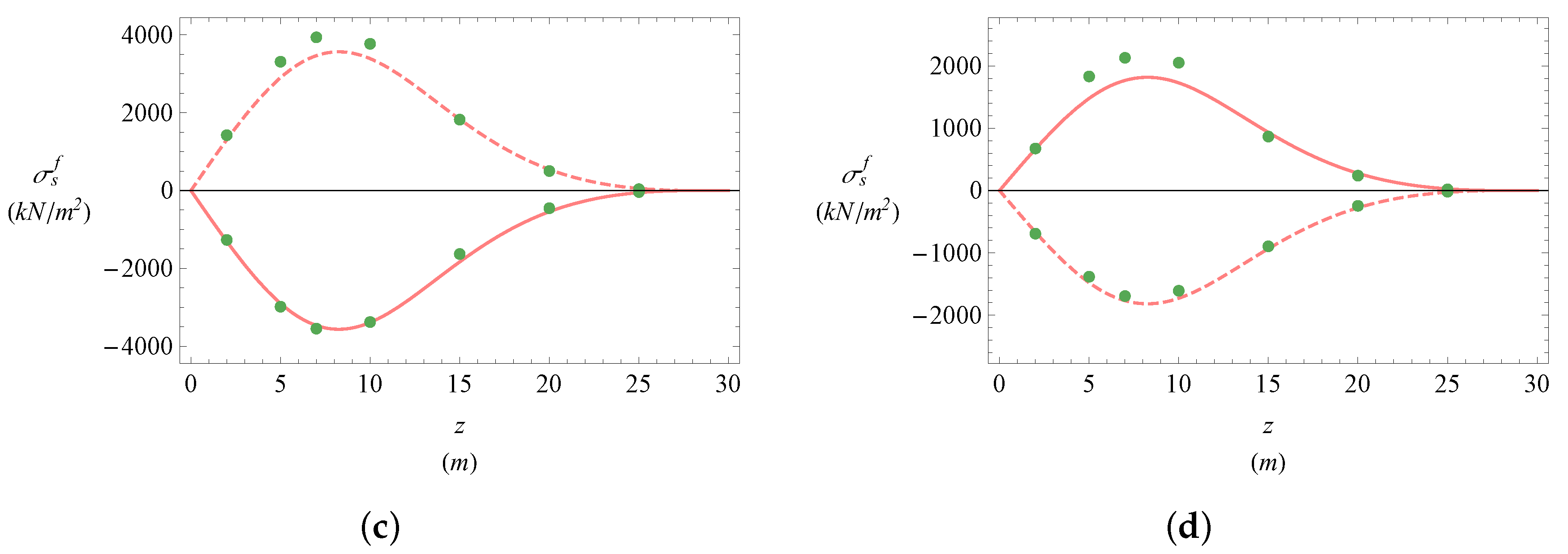
5.1.2. Stress Analysis in Torsion–Distortion

The complete analytical solution ( θ 0 ,   φ 0 ) is now considered, and relevant stresses (Equations (26) and (27)) are compared with those furnished by the unconstrained FE model. The membrane longitudinal normal stresses at the corners, σ z m z , b 2 , σ z m z , h 2 , are plotted in Figure 19a,b; they are found to be in excellent agreement with FEM analysis. Moreover, they are about three times larger that the normal stresses induced by torsion alone (Figure 17), thus highlighting the role of warping by distortion. The membrane tangential stresses at half side, τ m z , s 1 = 0 , τ m z , s 2 = 0 , are plotted in Figure 19c,d. Here, the contributions of active and reactive parts, together with their sum, are displayed. It is seen that the reactive component associated with distortion is essential, as discussed before, to achieve a good agreement with the numerical results. Finally, the maximum flexural tangential stresses at half side τ f z , s 1 = 0 , y 1 = t 1 2 and τ f z , s 2 = 0 , y 2 = t 2 2 are plotted in Figure 19e,f, showing, again, an excellent accordance between analytical and numerical results. The flexural component of the tangential stress is found to be comparable or even larger than the membrane component, thus revealing the importance to consider the variation in stresses inside the thickness of the cross section of reinforced concrete bridges.
The transverse normal stresses, mainly related to the distortion, are reported in Figure 20. Stresses acting at the cross section z = 7.5   m are displayed in Figure 20a,b. The linear law predicted by the analytical model is confirmed by FEM to within an error of about 10% at corners. When the variation with z of the stresses at corners was analyzed (Figure 20c,d), a 10% error is confirmed just in the region loaded, while the error almost vanishes far from this zone. As a curiosity, while the analytical model predicts the same absolute values for the stresses at the two faces, the FEM analysis reveals slight differences, more significant on one of the two faces. The reactive transverse normal stresses, which are associated with the normal forces induced by the bending moments, were checked as an attempt to explain this discrepancy, but they were found to be negligibly small. Therefore, such a phenomenon cannot be captured by the unique distortion mode considered here. Moreover, further investigation would be needed to unfold the effects of the way the external loads are applied to the box-girder, which, according to the De Saint Venant principle, are not negligible close to the loaded region.
As a final comment, it is important to notice that the distortional stresses in Figure 19 and Figure 20 are of the same order of magnitude or larger than the stresses due to pure torsion in Figure 16 and Figure 17. Therefore, distortion plays an important role in this sample system.

6. Conclusions

A minimal linear and elastic model of rectangular box-girder, undergoing twist and distortion, was formulated in the framework of GBT. The model is useful for bridge analysis in skew-symmetric loading conditions caused by the eccentricity of live loads. The displacement field was approximated as the superposition of two cross-sectional modes, one describing twist and the other describing distortion, all given in closed form. Modes are modulated by two amplitude functions, defined on the beam axis, governed by a set of two coupled fourth-order ordinary differential equations, which generalize the well-known uncoupled equations by Vlasov for torsion and of beam on elastic soil for distortion. The method, being analytic, is able to supply closed-form expressions for stresses in the whole domain.
Algorithmic aspects related to these equations were tackled, leading to the following conclusions.
  • The coefficients of the derivatives of fourth-order are mainly generated by nonuniform warping both in twist and distortion. Therefore, among them, the contribution of the flexural nature of the plates are negligible. In contrast, warping terms, although small, cannot be neglected when the displacement wavelength is short. It is argued that they could be relevant in describing boundary layers, e.g., produced by constraints preventing free warping.
  • The distortion-to-twist ratio was proven to be of order 1 for thin and short girders.
  • The Fourier analysis is a convenient and efficient tool to analyze simply supported girders warping free at the ends; for other boundary conditions, exact integration of the differential equations should be carried out. By following the literature, a simplified procedure was illustrated, which calls for neglecting all coupling terms, solving two independent problems and superimposing the effects. The two problems are (i) the Vlasov beam under torsion and (ii) the Winkler soil equation-like beam for distortion.
A sample system was considered, for which both Fourier analysis and uncoupled equation integration were carried out. The following conclusions were drawn.
  • Fourier analysis works well even for non-smooth loading conditions, provided that a sufficient number of terms is accounted for in the series. The exact integration of the uncoupled equations gives reasonably good results, with errors of about 10% with respect to the coupled Fourier representation.
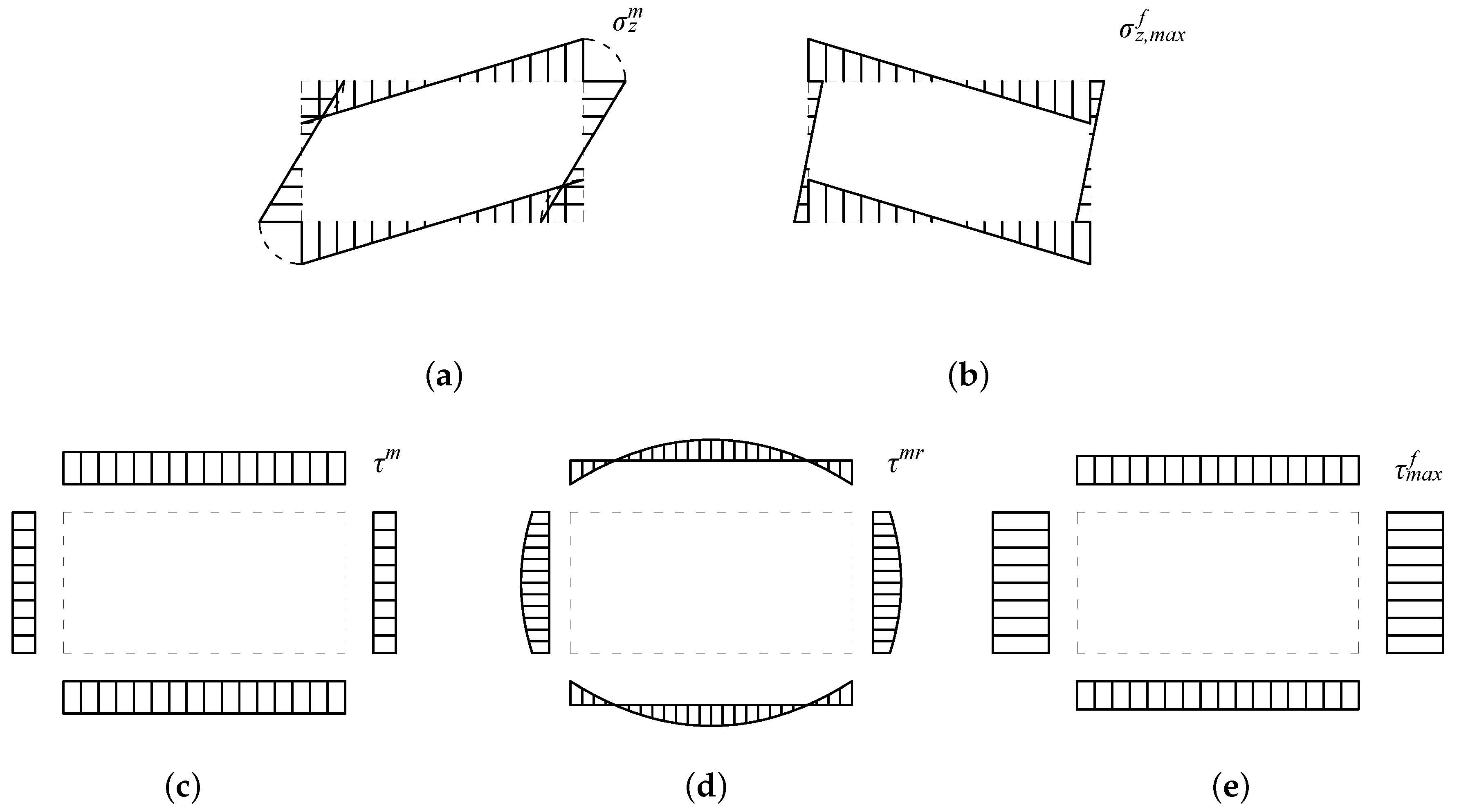
  • Stresses due to torsion mainly consist of (i) normal longitudinal components equilibrating the bimoment; (ii) active tangential stresses, as given by the Bredt theory; and (iii) reactive tangential stresses equilibrating the complementary torsional moment due to warping. All these effects are significant, except for the reactive tangential stresses, of which the influence is appreciable only close to the discontinuity points of the load.
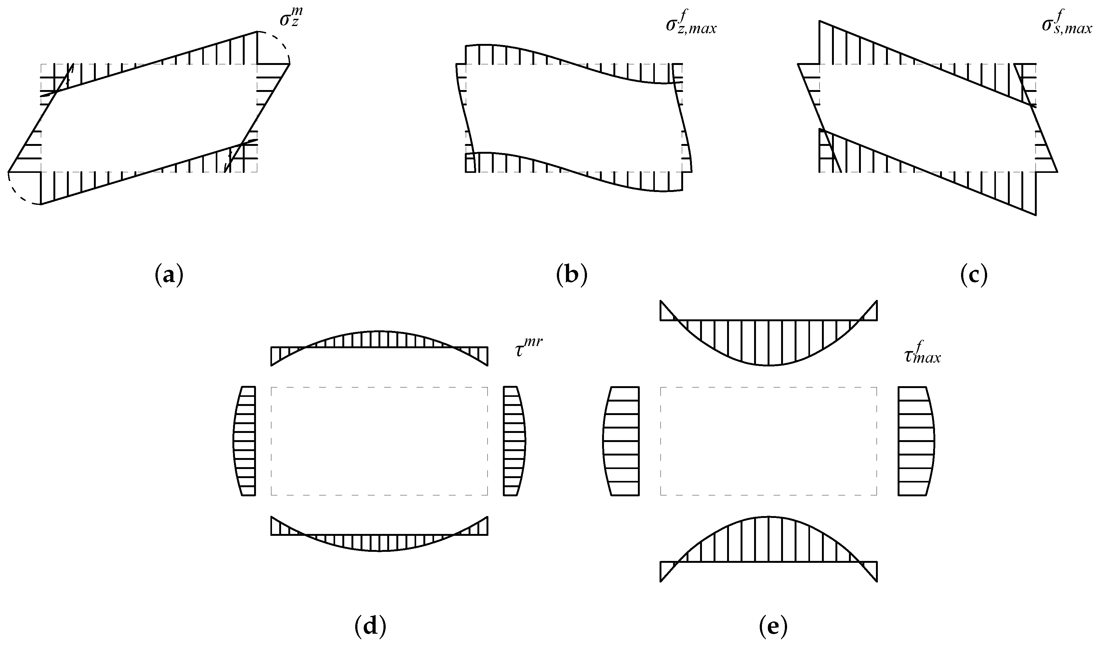
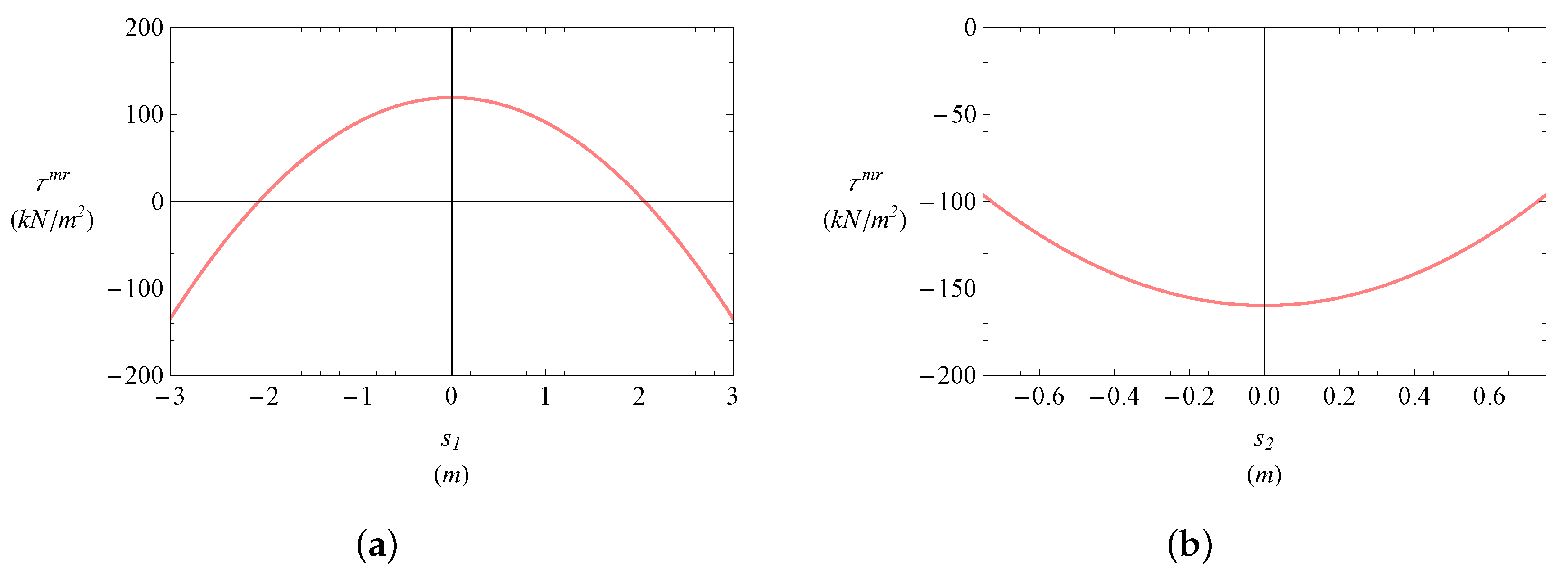
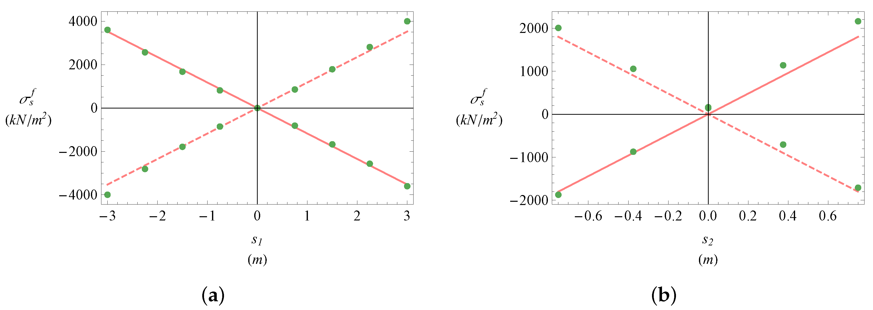
  • Stresses due to distortion consist of (i) membrane normal stress in the longitudinal direction, triggered by nonuniform warping, kinematically compatible with the loss of the shape of the cross section; (ii) membrane normal stresses in the transverse direction, generated by the frame-like behavior of the cross-section; (iii) flexural normal stresses in the longitudinal direction, generated by the flexure of the plates associated with the longitudinal modulation of the frame-deflection; and (iv) tangential stresses, generated by the torsion of the plates, made of an active and a reactive component. Among these stresses, (i) and (ii) are the most important. However, among the tangential stresses, the reactive component cannot be neglected.
Finally, all the results have been validated by a Finite Element Analysis. In spite of a remarkably larger computational effort, the differences between numerical and analytical results were found to be small. It is therefore confirmed that the simple analytical model proposed here is able to capture, with acceptable precision, the mechanical behavior of the girder.
The research is susceptible to some extensions. In the static field, (i) the exact solution of the two coupled equation could be found and more complicated boundary conditions could be analyzed and (ii) a one-dimensional finite element could be formulated to account for highly segmented or lumped loads as well for multi-span bridges. In the dynamic field, (iii) the free and forced vibrations of box-girder in torsion–distortion could be analyzed.

Author Contributions

Conceptualization, A.L.; methodology, A.L.; software, F.P.; validation, F.P.; formal analysis, A.L.; investigation, F.P.; resources, A.L. and F.P.; data curation, F.P.; writing—original draft preparation, A.L.; writing—review and editing, A.L. and F.P.; visualization, F.P.; supervision, A.L.; project administration, A.L. All authors have read and agreed to the published version of the manuscript.

Funding

This research received no external funding.

Conflicts of Interest

The authors declare no conflict of interest.

Appendix A. The Vlasov Stresses in Rectangular Box-Girders under Nonuniform Torsion

The rectangular box-girder in Figure 1 was considered, and stresses due to nonuniform torsion were calculated according to the Vlasov theory. The warping function (Equation (1)) is as follows:
ω s = 1 2 b t 2 h t 1 b t 2 + h t 1 h s i i = 1 , 3 1 2 b t 2 h t 1 b t 2 + h t 1 b s i i = 2 , 4
from which the warping inertia I ω = Γ ω 2 s t s d s is computed as follows:
I ω = b 2 h 2 24 h t 1 b t 2 2 b t 1 + h t 2 h t 1 + b t 2 2
The normal stresses are evaluated via σ z z , s = B z I ω ω s , with B z = E θ ( z ) , thus obtaining the following:
σ z z , s = E θ ( z ) h 2 b t 2 h t 1 b t 2 + h t 1 s i i = 1 , 3 E θ ( z ) b 2 b t 2 h t 1 b t 2 + h t 1 s i i = 2 , 4
The active tangential stresses (indexes omitted) are given by the Bredt formula τ a z , s = M t z G Ω 0 t s , with M t z = G J θ ( z ) , Ω 0 = b h and J = 4 ( b h ) 2 2 b t 1 + h t 2 , leading to the following:
τ a z , s = G b h t 2 h t 1 + b t 2 θ ( z ) i = 1 , 3 G b h t 1 h t 1 + b t 2 θ ( z ) i = 2 , 4
The reactive tangential stresses τ r z , s must be evaluated by integrating the indefinite equilibrium equation τ r t , s + σ z t , z = 0 . By accounting for σ z , z = E θ z ω s and remembering that t s is step-wise constant, it follows that τ r z , s i = 0 s ω s i d s i + c i E θ z , i.e.,
τ r z , s i = 1 4 b t 2 h t 1 b t 2 + h t 1 h s i 2 + c 1 E θ z i = 1 , 3 1 4 b t 1 h t 2 b t 2 + h t 1 b s i 2 + c 2 E θ z i = 2 , 4
where c 1 , c 2 are arbitrary constants. By enforcing the continuity of the flow at joints, i.e., t 1 τ r z , s 1 = b 2 = t 2 τ r z , s 2 = h 2 , and the equivalence of the reactive stresses to M t x = E I ω θ , i.e.,
h b / 2 b / 2 τ r z , s 1 t 1 d s 1 + b h / 2 h / 2 τ r z , s 2 t 2 d s 2 = E I ω θ
a linear system in the two unknown constants is derived:
t 1 t 2 t 1 t 2 c 1 c 2 = 1 b h E 1 16 b 2 h 2 β b t 1 + h t 2 I ω + 1 48 b 2 h 2 β b t 1 h t 2
By solving for c 1 , c 2 and coming back to Equation (A5), Equation (25) is found. It should be noticed that, if h b = t 2 t 1 , it is M t = 0 , then τ z s r z , s 0 .

Appendix B. Planar Frame Deflections

The rectangular planar frame in Figure 4 was considered with prescribed displacements at joints caused by the known distortion φ = 1 and with the rotations α unknowns. For a single beam, the stiffness matrix links shear forces and couples to displacements and rotations at the A , B ends:
V i M A V B M B = E I i 12 l i 3 6 l i 2 12 l i 3 6 l i 2 6 l i 2 4 l i 6 l i 2 2 l i 12 l 3 6 l i 2 12 l i 3 6 l i 2 6 l i 2 2 l i 6 l i 2 4 l i v A θ A v B θ B
with l i = b , h and I i = t 1 3 12 , t 2 3 12 , when i = 1 , 3 and i = 2 , 4 , respectively. It turns out that
  • when i = 1 , 3 , v A = b 2 v B = b 2 , θ A = θ B = α , entailing M A = M B = 6 E I 1 b + 6 E I 1 b α ;
  • when i = 2 , 4 , v A = h 2 and v B = h 2 , entailing M A = M B = 6 E I 2 h + 6 E I 2 h α .
Enforcing equilibrium at any joint (all the equilibrium conditions being equal for symmetries), it follows that
6 E I 1 b α 1 + 6 E I 2 h α + 1 = 0
from which α is derived, as given in Equation (16). To evaluate the deflections of each beam, the elastic line equation E I i V i s = 0 is integrated under the prescribed displacements at the end; namely
  • when i = 1 , 3 , V b 2 = b 2 , V b 2 = α , from which V i = 1 2 s i 3 + 4 s i 2 α 1 b 2 α
  • when i = 2 , 4 , V h 2 = ± h 2 , V b 2 = α , from which V i = 1 2 s i 3 + 4 s i 2 α + 1 h 2 α

Appendix C. Matrices in the GBT Equation (22)

By performing integrations in Equation (21), with the modes given by Equations (13), (15), (17), and (19), the following expressions are found for the GBT matrices:
  • Matrix C e :
    C e = E I ω 1 1 β 1 β 1 β 2
    where β is the warping ratio (Equation (20)) and I ω = b 2 h 2 24 h t 1 b t 2 2 b t 1 + h t 2 h t 1 + b t 2 2 = β 2 b 2 h 2 24 b t 1 + h t 2 is the warping stiffness. As already observed, when h b = t 2 t 1 , C 11 e = C 21 e = C 12 e = 0 while C 22 e 0 .
  • Matrix C f :
    C 11 f = E 72 b 3 t 1 3 + h 3 t 2 3 C 12 f = C 21 f = E 360 b 3 t 1 3 6 + α + h 3 t 2 3 6 + α C 22 f = E 2520 b 3 t 1 3 51 + 2 α 9 + α + h 3 t 2 3 51 + 2 α 9 + α
    where α (Equation (16)) is the joints’ distortional rotation.
  • Matrix D s :
    D s = G J 0 0 0
    where J = 4 ( b h ) 2 2 b t 1 + h t 2 is the Bredt torsional stiffness.
  • Matrix D t :
    D 11 t = 2 3 G b t 1 3 + h t 2 3 D 12 t = D 21 t = 2 3 G b t 1 3 h t 2 3 D 22 t = 2 15 G b t 1 3 6 + 2 + α α + h t 2 3 6 + α 2 + α
  • Matrix B f :
B f = 0 0 0 B 22 f , B 22 f : = 2 E b h t 1 3 h α 1 2 + t 2 3 b α + 1 2

Appendix D. Reactive Distortional Tangential Stresses

The membrane reactive tangential stresses τ m r z , s associated with the distortion of the cross section must be evaluated by integrating the indefinite equilibrium equation τ m r t s + σ z t , z = 0 . By using Equation (26) for σ z and integrating it, it follows that
τ m r z , s i = c i 1 4 E h s i 2 φ ( z ) i = 1 ,   3 c i + 1 4 E b s i 2 φ ( z ) i = 2 ,   4
where c i is an arbitrary constant. By enforcing equilibrium at the joints, i.e., t 1 τ r z , s 1 = b 2 = t 2 τ r z , s 2 = h 2 , and by imposing the tangential stresses are self-equilibrated, i.e.,
h b / 2 b / 2 τ r z , s 1 t 1 d s 1 + b h / 2 h / 2 τ r z , s 2 t 2 d s 2 = 0
an algebraic linear system for the constant follows:
t 1 t 2 t 1 t 2 c 1 c 2 = E b h 16 b t 1 + h t 2 b t 1 h t 2 3
By solving it and coming back to Equation (A15), Equation (27) is found.

References

  1. Vlasov, V.Z. Thin-Walled Elastic Beams; Monson: Jerusalem, Israel, 1961. [Google Scholar]
  2. Wright, R.H.; Abdel-Samuel, S.R.; Robinson, A.R. BEF Analogy for Analysis of Box-Girders. J. Struct. Div. ASCE 1968, 94, 1179–1743. [Google Scholar]
  3. Petrangeli, M.P.; Zechini, A. Il calcolo dei ponti a cassone unicellulare con pareti sottili. Giornale del Genio Civile 1973, 2, 108–122. [Google Scholar]
  4. Stefanou, G.D.; Dritsos, S.; Bakas, G.J. The effects of additional deformations in box-beam bridges on the longitudinal stresses and transverse moments. Comput. Struct. 1983, 16, 613–628. [Google Scholar] [CrossRef]
  5. Arici, M.; Granata, M.; Recupero, A. BEF Analogy for Concrete Box Girder Analysis of Bridges. In Proceedings of the 34th International Symposium on Bridge and Structural Engineering, Venice, Italy, 22–24 September 2010. [Google Scholar]
  6. Stavridis, L.T.; Spiliopoulos, K.V.; Afantenou, A.V.; Kapogiannis, I.A. Appraisal of simplified methods for the analysis of box-girder bridges. Int. J. Bridge Eng. 2015, 3, 55–64. [Google Scholar]
  7. Ren, Y.; Cheng, W.; Wang, Y.; Chen, Q.; Wang, B. Distortional analysis of simply supported box girders with inner diaphragms considering shear deformation of diaphragms using initial parameter method. Eng. Struct. 2017, 145, 44–59. [Google Scholar] [CrossRef]
  8. Mentrasti, L. Distortion (and Torsion) of Rectangular Thin-Walled Beams. Thin Wall Struct. 1990, 10, 175–193. [Google Scholar] [CrossRef]
  9. Mentrasti, L. Torsion of Box Girders with Deformable Cross Sections. J. Eng. Mech. 1991, 117, 2179–2200. [Google Scholar] [CrossRef]
  10. Sapountzakis, E.; Argyridi, A. Influence of in-plane deformation in higher order beam theories. J. Mech. Eng. 2018, 68, 77–94. [Google Scholar] [CrossRef] [Green Version]
  11. Zulli, D. A one-dimensional beam-like model for double-layered pipes. Int. J. Nonlinear Mech. 2019, 109, 50–62. [Google Scholar] [CrossRef]
  12. Zulli, D.; Casalotti, A.; Luongo, A. Static Response of Double-Layered Pipes via a Perturbation Approach. Appl. Sci. 2021, 11, 886. [Google Scholar] [CrossRef]
  13. Luongo, A.; Zulli, D. A non-linear one-dimensional model of cross-deformable tubular beam. Int. J. Nonlinear Mech. 2014, 66, 33–42. [Google Scholar] [CrossRef]
  14. Gabriele, S.; Rizzi, N.; Varano, V. A 1D nonlinear TWB model accounting for in plane cross-section deformation. Int. J. Solids Struct. 2016, 94–95, 170–178. [Google Scholar] [CrossRef]
  15. Ziane, N.; Ruta, G.; Meftah, S.A.; Doula, M.H.; Benmohammed, N. Instances of mixed buckling and post-buckling of steel RHS beams. Int. J. Mech. Sci. 2021, 190, 106013. [Google Scholar] [CrossRef]
  16. Cheung, Y.K. Finite Strip Method in Structural Analysis; Pergamon Press: Oxford, UK, 1976. [Google Scholar]
  17. Friedrich, R. Finite strip method: 30 Years—A bibliography (1968–1998). Eng. Comput. 2000, 17, 92–111. [Google Scholar] [CrossRef]
  18. Adany, S.; Schafer, B.W. A full modal decomposition of thin-walled, single-branched open cross-section members via the constrained finite strip method. J. Constr. Steel Res. 2008, 64, 12–29. [Google Scholar] [CrossRef]
  19. Schardt, R. Verallgemeinerte Technicsche Biegetheorie; Springer: Berlin/Heidelberg, Germany, 1989. [Google Scholar]
  20. Chidolue, C.A.; Osadebe, N.N. Flexural Torsional Behaviour of Thin Walled Mono Symmetric Box Girder Structures. Int. J. Eng. Sci. Emerg. Technol. 2012, 2, 11–19. [Google Scholar]
  21. Davies, J.M.; Leach, P.; Heinz, D. Second-Order Generalised Beam Theory. J. Constr. Steel Res. 1994, 31, 221–241. [Google Scholar] [CrossRef]
  22. Leach, P. The Calculation of Modal Cross-Section Properties for use in the Generaliszd Beam Theory. Thin Wall Struct. 1994, 19, 61–79. [Google Scholar] [CrossRef]
  23. Silvestre, N.; Camotim, D. First-order generalised beam theory for arbitrary orthotropic materials. Thin Wall Struct. 2002, 40, 755–789. [Google Scholar] [CrossRef]
  24. Gonçalves, R.; Ritto-Correa, M.; Camotim, D. A new approach to the calculation of cross-section deformation modes in the framework of generalized beam theory. Comput. Mech. 2010, 46, 759–781. [Google Scholar] [CrossRef]
  25. Bebiano, R.; Gonçalves, R.; Camotim, D. A cross-section analysis procedure to razionalise and automate the performance of GBT-based structural analyses. Thin Wall Struct. 2015, 92, 29–47. [Google Scholar] [CrossRef]
  26. Ferrarotti, A.; Piccardo, G.; Luongo, A. A novel straightforward dynamic approach for the evaluation of extensional modes within GBT ’cross-section analysys’. Thin Wall Struct. 2017, 114, 52–69. [Google Scholar] [CrossRef]
  27. Ranzi, G.; Luongo, A. A new approach for thin-walled member analysis in the framework of GBT. Thin Wall Struct. 2011, 49, 1404–1414. [Google Scholar] [CrossRef] [Green Version]
  28. Piccardo, G.; Ranzi, G.; Luongo, A. A complete dynamic approach to the Generalized Beam Theory cross-section analysis including extension and shear modes. Math. Mech. Solids 2014, 19, 900–924. [Google Scholar] [CrossRef]
  29. Piccardo, G.; Ranzi, G.; Luongo, A. A direct approach for the evaluation of the conventional modes within the GBT formulation. Thin Wall Struct. 2014, 74, 133–145. [Google Scholar] [CrossRef]
  30. Taig, G.; Ranzi, G.; D’Annibale, F. An unconstrained dynamic approach for the Generalised Beam Theory. Continuum Mech. Therm. 2015, 27, 879–904. [Google Scholar] [CrossRef]
  31. de Miranda, S.; Gutierrez, A.; Miletta, R.; Ubertini, F. A generalized beam theory with shear deformation. Thin Wall Struct. 2014, 67, 88–100. [Google Scholar] [CrossRef]
  32. de Miranda, S.; Madeo, A.; Miletta, R.; Ubertini, F. On the relationship of the shear deformable Generalized Beam Theory with classical and non-classical theories. Int. J. Solids Struct. 2014, 51, 3698–3709. [Google Scholar] [CrossRef] [Green Version]
  33. Bianco, M.J.; Habtemariam, A.K.; Knke, C.; Zabel, V. Analysis of warping and distortion transmission in mixed shell–GBT (generalized beam theory) models. Int. J. Adv. Struct. Eng. 2019, 11, 109–126. [Google Scholar] [CrossRef] [Green Version]
  34. Manta, D.; Gonçalves, R.; Camotim, D. Combining shell and GBT-based finite elements: Linear and bifurcation analysis. Thin Wall Struct. 2020, 152, 106665. [Google Scholar] [CrossRef]
  35. Dikaros, I.C.; Sapountzakis, E.J. Distortional Analysis of Beams of Arbitrary Cross Section Using BEM. J. Eng. Mech. 2017, 143, 04017118. [Google Scholar] [CrossRef]
  36. Silvker, V. Closed-profile thin-walled bars—A theory by Umanski. In Mechanics of Structural Elements-Theory and Applications; Springer: Berlin/Heidelberg, Germany, 2007; pp. 395–432. [Google Scholar]
  37. Schardt, R. Generalized Beam Theoy—An Adequate Method for Coupled Stability Problems. Thin Wall Struct. 1994, 19, 161–180. [Google Scholar] [CrossRef]
Figure 1. Box-girder: (a) geometry; (b) element numbering and local systems of coordinates.
Applsci 11 02501 g001
Figure 2. Decomposition of the cross-sectional transformation: (a) current configuration, (b) skew-symmetric part (twist), and (c) symmetric part (distortion). Compatibility at corners to be accounted for later.
Applsci 11 02501 g002
Figure 3. Torsional mode: (a) tangential displacements, (b) normal displacements, and (c) warping.
Applsci 11 02501 g003
Figure 4. Distortional deflection: (a) translating joints, (b) rotating joints, and (c) superposition of displacements.
Applsci 11 02501 g004
Figure 5. Distortional mode: (a) tangential displacements, (b) normal displacements, and (c) warping.
Applsci 11 02501 g005
Figure 6. Warping ratio β = W t W d vs. the aspect ratio b h for different thickness ratios t 1 t 2 .
Applsci 11 02501 g006
Figure 7. Stresses in the torsional mode: (a) membrane longitudinal normal stress, (b) flexural longitudinal normal stress, (c) active membrane tangential stress, (d) reactive membrane tangential stress, and (e) flexural tangential stress. (b,e) the index max denotes evaluation at the top/bottom face of the plates (i.e., at y i = ± t i 2 ).
Applsci 11 02501 g007
Figure 8. Stresses in the distortional mode: (a) membrane longitudinal normal stress, (b) flexural longitudinal normal stress, (c) flexural transverse normal stress, (d) membrane reactive tangential stresses, and (e) flexural tangential stress. (b,c,e) the index max denotes evaluation at the top/bottom face of the plates (i.e., at y i = ± t i 2 ).
Applsci 11 02501 g008
Figure 9. Flexural-to-extensional coefficient ratios vs. the height-to-thickness ratio for different b h aspect ratios: (a) C 11 f C 11 e , (b) C 12 f C 12 e , (c) C 22 f C 22 e vs. h t ; t 2 t 1 = 1 .
Applsci 11 02501 g009
Figure 10. Influence of the fourth-order terms on the sinusoidal solution: (ac) extensional-to-shear ratios r i j s : = C i j e G J n π 2 ; (df) extensional-to-flexural ratios r i j f : = C i j e B 22 f n π 4 vs. the squatness ratio n h for different aspect ratios b h ; h t 1 = 6 (black dashed lines), and h t 1 = 8 (gray continuous lines); t 2 = 1.4 t 1 .
Applsci 11 02501 g010
Figure 11. Distortion-to-twist ratio vs. the thickness-to-height ratio for different slenderness ratios n h : (a) squared box b = h ; (b) rectangular box b h = 4 ; t 1 = t 2 = : t .
Applsci 11 02501 g011
Figure 12. Segment of distributed load, p 0 = ± P Δ , centered at z = ξ : (a) longitudinal view; (b) cross section at z = ξ , dimensions in meters.
Applsci 11 02501 g012
Figure 13. Fourier coefficients and truncated series for (a) loads, (b) twist angle, and (c) distortion.
Applsci 11 02501 g013
Figure 14. Comparison among deflections: (a) twist angle, (b) distortion; Fourier ( N = 50 terms, thick red lines), Finite Element Method (FEM) (bullets), and uncoupled differential equations (thin gray lines).
Applsci 11 02501 g014
Figure 15. Derivatives of deflections: (a,c,e) twist angle derivatives, (b,d,f) distortion derivatives; comparison between Fourier ( N = 50 terms, thick red lines) and uncoupled solutions to the differential equations (thin gray lines).
Applsci 11 02501 g015aApplsci 11 02501 g015b
Figure 16. Torsion without distortion: longitudinal normal stresses and tangential stresses at the cross section z = 7.5   m vs. s i ; bottom edge (continuous line), top edge (dashed lines); (a,b) σ z , m a x m + f : = σ z m + σ z , m a x f ; (c,d) τ m a x m + f : = τ m + τ m a x f ; (a,b) element 1, (c,d) element 2. Fourier analysis with N = 50 terms, FEM analysis (bullets).
Applsci 11 02501 g016
Figure 17. Torsion without distortion: longitudinal normal σ z , m a x m + f : = σ z m + σ z , m a x f and tangential τ m a x m + f : = τ m + τ m a x f stresses, at corners ( s i = b 2 , h 2 ) and top face (dashed lines) and bottom face (continuous lines ) vs. z; (a,b) element 1, (c,d) element 2; Fourier analysis with N = 50 terms; FEM analysis (bullets).
Applsci 11 02501 g017
Figure 18. Torsion without distortion: Reactive tangential stresses τ m r at z = 11.25   m vs. s i : (a) element 1, (b) element 2.
Applsci 11 02501 g018
Figure 19. Torsion coupled to distortion: (a,b) membrane longitudinal normal stresses evaluated at the corners ( s i = b 2 , h 2 ); (c,d) active (dashed black line), reactive (blue line), and total (red line) membrane tangential stresses evaluated at half side ( s i = 0 ); (e,f) flexural tangential stresses evaluated at half side ( s i = 0 ) bottom/top edge ( y i = t i 2 ); (a,c,e) element 1, (b,d,f) element 2; Fourier analysis with N = 50 terms, FEM analysis (bullets).
Applsci 11 02501 g019
Figure 20. Torsion coupled to distortion: (a,b) Transverse normal stresses at bottom edges (continuous lines) and top edges (dashed lines): (a,b) stresses at z = 7.5   m vs. s i , (c,d) stresses at the corners vs. z; (a,c) element 1, (b,d) element 2. Fourier analysis with N = 50 terms, FEM analysis (bullets).
Applsci 11 02501 g020aApplsci 11 02501 g020b
Table 1. Coefficients of the Generalized Beam Theory (GBT) equations.
(i,j)(1,1)(1,2)(2,2)
C i j e 1.18 × 10 8 1.70 × 10 8 2.44 × 10 8
C i j f 1.74 × 10 6 2.21 × 10 6 3.29 × 10 6
D i j s 1.02 × 10 8 00
D i j t 1.88 × 10 6 3.50 × 10 5 2.63 × 10 6
B i j f 00 6.80 × 10 5
Publisher’s Note: MDPI stays neutral with regard to jurisdictional claims in published maps and institutional affiliations.

