Prediction of Model Distortion by FEM in 3D Printing via the Selective Laser Melting of Stainless Steel AISI 316L

Abstract

This paper deals with an experimental analysis of stress prediction and simulation prior to 3D printing via the selective laser melting (SLM) method and the subsequent separation of a printed sample from a base plate in two software programs, ANSYS Addictive Suite and MSC Simufact Additive. Practical verification of the simulation was performed on a 3Dprinted topologically optimized part made of AISI 316L stainless steel. This paper presents a typical workflow for working with metallic 3D printing technology and the state-of-the-art knowledge in the field of stress analysis and simulation of printed components. The paper emphasizes the role of simulation software for additive production and reflects on their weaknesses and strengths as well, with regard to their use not only in science and research but also in practice.

1. Introduction

The 3D printing (additive manufacturing (AM)) of precise metal models includes three technological phases: pre-process (simulation, prediction, and data preparation), processing (3D printing), and post-processing (heat treatment, support removal, machining, etc.). These processes can realize a significant reduction in or even elimination of stresses and deformations, thereby reducing scrap and manufacturing costs. Selective laser melting (SLM) is a powder bed fusion (PBF) additive manufacturing technology, whose principle consists of melting atomized metal powder by laser. The SLM method is characterized by a thermal process taking place in the so-called melt pool, where the metal powder melts [1]. Due to the repeated heating and cooling, there are high temperature gradients resulting in high thermal stress in SLM-printed parts [2]. Heat transfer in the SLM process has a great influence on the final mechanical properties of the print. To obtain a fully dense component without pores, it is necessary to completely melt the metallic particles of the powder. Therefore, it is advisable to use high laser power. However, this power can produce negative thermal effects, such as the balling effect and internal stress [3], causing part distortion or cracks.

Several researchers have already studied distortion prediction [4,5], mostly based on simulations of a model for welding using the finite elements (FE). This simulation method involves the application of a mathematically modeled heat source to the thermomechanical finite element analysis (FEA) [4]. This method has been mainly applied in a process where the input material is a powder or an additional wire. However, these simulations are very limited when the geometry of the part is complex. Chiumenti et al. [5] performed a fully coupled thermo-mechanical numerical simulation that included phase-change phenomena defined in terms of both the latent heat release and shrinkage effects. In this way, the authors formulated a new activation methodology for simulating layer deposition. This method was followed by the work of Lundbäck et al. [6], who successfully simulated the deposition of individual layers. In addition, the authors improved the model by calibrating the inflow and heat input to predict the correct temperature and distortion. The authors then compared the results experimentally. Hussein et al. [7] developed a 3D FE model for the prediction of melt pool size and temperature gradients that are affected by the scan speed parameter during single-layer deposition. This model, however, is valid only for AISI 316L materials. The authors noted that higher speeds produced a smaller melt pool size based on the width and depth parameters, but the pool length parameter was higher. Another conclusion of this publication was that the highest temperature gradients were reached with the first layer and then rapidly decreased with each subsequent layer (at all scan speeds tested). Zhang et al. [8] used a 3D FE model to investigate the dependence of temperature gradients on laser power and scanning speeds. It was shown that high laser power and low scanning speed led to significant heat input and a high maximum temperature in the SLM process. However, these simulation approaches require high computer (PC) performance and considerable computational time. To speed up the simulations, some researchers have begun to use the inherent strain approach, which is commonly employed in the field of welding for large components. Keller et al. [9] used the inherent strain approach at a macroscale and successfully managed to significantly reduce the computational times of the simulations. However, it remains unknown how accurate these simulations are, because they have not been experimentally verified. A similar approach based on FE and inherent strain was developed by the team of Afazov et al. [10], who succeeded in simulating an industrial model of an impeller blade at a macroscale. The data obtained from the simulation were successfully experimentally verified with a high degree of accuracy. Song et al. [11] noted that for an accurate simulation, it is necessary to consider the powder surrounding the printed part, given that the heat is transferred through supports to the base plate and the surrounding powder insulates the heat.

To verify the accuracy of the simulation, the results need to be experimentally verified, i.e., one needs to print the part and then measure its deformed state. There are several methods for this. One of the most widely used and non-destructive methods is 3D scanning, which generally allows one to compare a model from a real scan at an accuracy up to 0.025 mm. Alternatively, 3D full-field measurements can be taken using the digital image correlation (DIC) method, which is a method for measurement that also captures deformations/strains on the visible part surface. The advantage of this method is that no contact with the investigated part is required. This method utilizes optical testers that measure not only displacements and strains but also velocities and accelerations on the vibrated part. The DIC method is currently also applied in hole-drilling residual stress measurements [12]. X-ray diffraction can also be used for non-destructive testing, but it can only light up a very relatively thin layer [13].

As listed above, although numerical studies of the printing process and its products have been investigated intensively, there are few studies that consider the thorough process from the designing stage to fabrication of the optimal components so as to bridge the gap between academic works and practice. In view of this, this study presents a typical workflow from designing to manufacturing and finally quality control (QC) of parts fabricated with the state-of-the-art SLM technology. In particular, a part was designed and topologically optimized. Subsequently, two commercially available software programs, namely ANSYS Addictive Suite and MSC Simufact, were utilized to evaluate the deformation of the optimized part caused by the printing process. For both cases, the 3D non-linear finite element model based on thermo-mechanical fields was presented and compared. Finally, the part went through the QC process conducted with DIC and 3D scanning methods. The surface deviation results from the two methods were collected and compared. The manuscript answers the following questions:

• What are the roles of simulation in preparation for the fabricating process with SLM technology? How accurate are they in predicting the dimensional deviation of the printed parts?
• How dimensionally accurate is the SLM-fabricated part in comparison with the Computer Aided Design (CAD) design?
• What are the controllable factors that need to be considered in the whole process to obtain dimensionally, functionally, and economically optimal SLM-fabricated parts?

2. Materials and Methods

Both ANSYS Additive Suite (AAS) and MSC Simufact work on the principle of finite element (FE) simulation and are directly designed for SLM technology. The primary task of these programs is to avoid unnecessary cost and time expenditures and improve product quality. Thanks to the prediction of stresses and deformations in the AM process, these tools allow one to choose the optimal design and orientation of the part in the build chamber. Another function is distortion prediction, which allows the part to be printed as pre-deformed to obtain the required geometry. Both simulation programs use layered discretization with voxel elements (a cube with a defined edge length). The AAS also offers layered tetrahedral elements for better adaptation to the shape of the part. In the AAS program, it is recommended to set 10–20 times the actual height of the print layer for layer simulation [14]. For MSC Simufact, the manual recommends setting the voxel size to 1.8 mm. According to the literature [15], the smaller the voxel size that is set, the longer the simulation will take. In general, the simulation procedure can be described by a flowchart in a similar way to Bian et al. in their research [16], as shown in Figure 1.

2.1. ANSYS Additive Suite

The AAS is fully adapted for work in the ANSYS Workbench environment. The component is first completely meshed with individual layers of either the voxel or tetrahedral elements. Each FE layer represents several real metal powder layers, assuming thermal continuity with the next layer. The program does not consider a moving heat source, such as when the thermal gradient in the build direction dominates over the thermal gradient in the plane direction due to its effect on residual deformations. Unlike MSC Simufact, the AAS requires more input parameters. To simulate the process, it is necessary to specify the basic properties of the material, which are temperature dependent. Inherent strain calibration, which simplifies the data input process, is as well possible, but the first approach with default values from the software’s database was considered in this study. These parameters include the elastic modulus, orthotropic thermal conductivity, Poisson’s ratio, density, elastic bilinear curves of the plastic stress and strain, the coefficient of thermal expansion, and the specific heat capacity up to the melting point of the material. In this study, the material properties for AISI 316L (AM), which is predefined in the ASS, were set for the simulation. The other process parameters necessary for print simulation are given in

Table 1. Process parameter for input data in ANSYS Additive Suite (AAS).

Parameter	Value
Element size	1 mm
Method	Cartesian
Hatch spacing	0.11 mm
Scan speed	650 mm/s
Laser power	200 W
Preheat temperature	22 °C
Layer thickness	50 µm
Scan strategy	Meander

. Meshing was also used to build a plate with a hexahedral element.

For this study, we used ANSYS Inc. ANSYS Mechanical Workbench, version 2020R1.

2.2. MSC Simufact

MSC Simufact is a program developed specifically for power bed fusion additive manufacturing simulations. Selective laser melting (SLM), electron beam melting (EBM), laser beam melting (LBM), and direct metal laser sintering (DMLS) methods can be analyzed. One of the advantages of this software is its simulation of the whole AM process, such as printing simulation, support cutting, heat treatment, hot isostatic pressing (HIP), and the evaluation of residual stresses and distortions. MSC Simufact offers only a hexahedral element for a voxel mesh. After creating the voxel mesh, a volumetric mesh structure is created, which provides a 3D network; then, a surface mesh is generated. The voxel and surface mesh complement each other and thus guarantee coverage of the entire part. Since the program offers an inherent strain calibration function, it is necessary to calibrate first the software with the real machine with the use of cantilevers following this approach. Specifically, a set of cantilevers was first printed on the printer in various positions and were then cut lengthwise, thus activating residual stresses and entering the measured values into the software. The material curves and constants were already predefined for the AISI 316L material, as well as for the AAS, by the manufacturer. The only necessary input from the user is the input of the machine type (for setting the working space), the layer thickness, the direction of cutting the part from the printing pad, and the voxel size.

For this study, we used MSC Software Inc. Simufact, version 2019. The main considered parameters in the simulation are outlined in

Table 2. Process parameters for input data in MSC Simufact.

Parameter	Value
Element size	1 mm
Method	Inherent Strains
Hatch spacing	0.11 mm
Scan speed	650 mm/s
Laser power	200 W
Preheat temperature	Ambient
Layer thickness	50 µm
Scan strategy	Meander

.

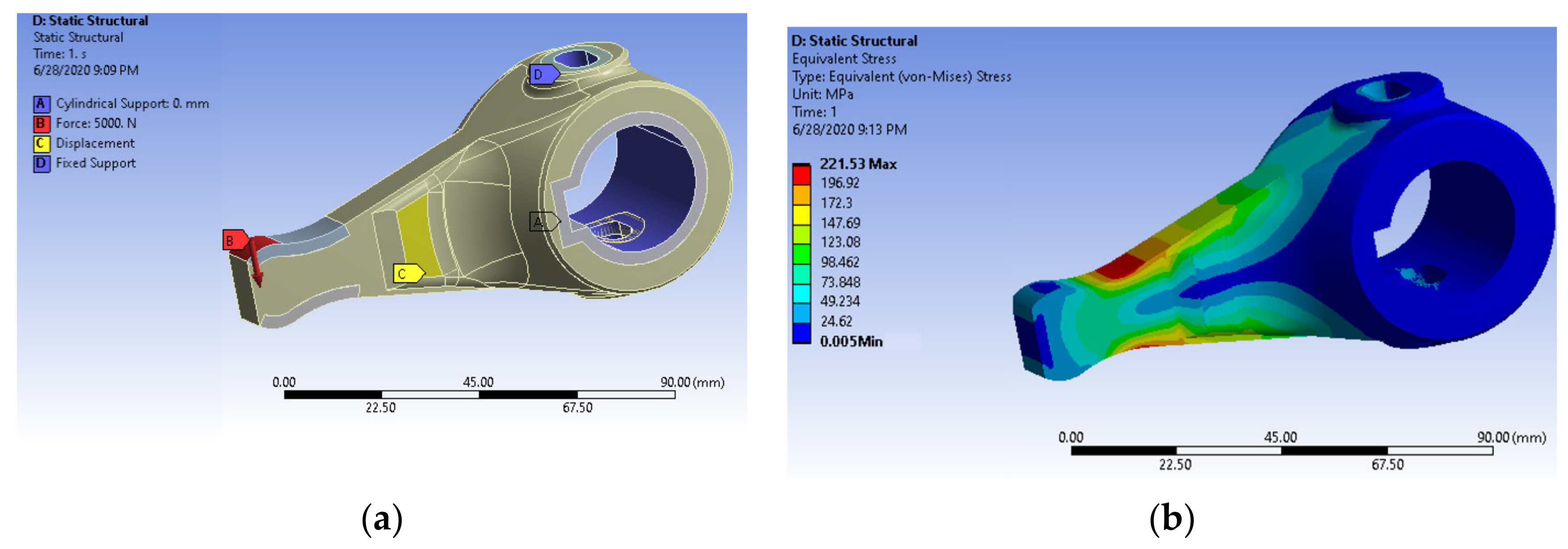
2.3. Topology Optimization

For evaluation and validation purposes, we chose a practical component called the shifting thumb (with dimensions 110 × 55 × 41 mm; see Figure 2), which is used as a mechanical-pneumatic power steering, on TATRA 14TS210L manual transmissions. The original shape was topologically optimized for maximum 3D printing potential (see Figure 3). The original model was subjected to a total force of 5000 N in the normal direction of the loaded face according to Figure 4a. Considered constraints are depicted in the same picture. Young’s modulus E = 195 GPa and Poisson’s ratio ν = 0.3 were used as elastic constants of stainless steel AISI 316L in all simulations. Initially, an FE elastostatic analysis in ANSYS Workbench was performed for the original geometry. As a result, von Mises stress contours obtained in the original part are presented in Figure 3b. The keyway is not used for transferring a torque, which is why there is no hotspot of stresses. The torque is transferred by two holes with faces depicted by mark D in Figure 4a. It should be noted that the topology optimization is done to cut off the weight from the part, while ensuring that the part is functional and with comparable stiffness in comparison to its original counterpart. Specifically, in our study, we saved 63% of weight (From Figure 3a to Figure 3b, 646 g to 236 g) and obtained comparable stiffness and stresses (Figure 4b vs. Figure 6, 222 MPa vs. 232 MPa/214 MPa) after topology optimization.

Topological optimization has become a powerful area of study since such algorithms can be applied to many design problems in different physical disciplines, such as solid mechanics, fluid dynamics, and thermal dynamics [18,19,20]. By using topological optimization methods and related algorithms, a designer can generate innovative design ideas, especially in engineering fields. Instead of using trial-and-error methods for designing engineering products, designers use different topological optimization methods to generate conceptual designs.

Topological optimization methods can be distinguished by two main methods: solid isotropic material with penalization, otherwise known as SIMP, and the level-set method. Each method has unique features, although both can be used to achieve similar goals. The SIMP method is the most popular due to its conceptual simplicity and computational efficiency. However, it requires more post-processing and smoothing due to its gray elements, which produce a rough surface geometry [21].

The mathematical representation of the SIMP method is based on the heuristic relationship between the relative element density x_i and the element of the Young’s modulus E_i given by

$$E_i= E_i\left(x_i\right)= x_i^p{E}_{0 }, x_i\in \left[0,1\right],$$

(1)

where $E_0$ is the elastic modulus of the solid material and $p$ is the penalization power $(p>1)$. A modified SIMP approach is given by

$$E_i=E_i\left(x_i\right)=E_{min}+x_i^p\left(E_0-E_{min}\right), x_i\in \left[0,1\right],$$

(2)

where $E_{min}$ is the elastic modulus of the void material, which is non-zero to avoid a singularity of the finite element stiffness matrix.

The modified SIMP approach offers several advantages over the classical SIMP formulation, including independency between the minimum values of the materials’ elastic modulus and superior penalization power [22].

However, topological optimization methods are likely to encounter numerical difficulties, such as mesh dependency, checkerboard patterns, and local minima [23]. To mitigate such issues, researchers have proposed the use of regularization techniques [24]. One of the most common approaches is the use of density filters [25].

On the other hand, the compliance function in the level-set method relies on the response type or constraint. Static structural analysis supports a combination of force-based and displacement-based loading, as well as thermal loading. The compliance function can be described as follows:

$$\begin{array}{c}J\left(\mathsf{\Omega }\right)=\frac{1}{2}\left[{{\displaystyle \int }}_{\mathsf{\Omega }}A\left(e\left(u\right)-e^{th}\right):e^{th}dx+{{\displaystyle \int }}_{\mathsf{\Omega }}f*udx+{{\displaystyle \int }}_{{\mathsf{\Gamma }}_N}g*uds+{{\displaystyle \int }}_{{\mathsf{\Gamma }}_u}{\lambda }_u*u_{0}ds\right]\\ =\left[-\frac{1}{2}{{\displaystyle \int }}_{\mathsf{\Omega }}A\left(e\left(u\right)-e^{th}\right):\left(e\left(u\right)-e^{th}\right)dx+{{\displaystyle \int }}_{\mathsf{\Omega }}f*udx+{{\displaystyle \int }}_{{\mathsf{\Gamma }}_N}g*uds\right]\end{array}$$

(3)

where $e\left(u\right)=\frac{1}{2}\left(\nabla u+{\left(\nabla u\right)}^t\right)$ is the total strain vector, $e^{th}$ is the thermal strain vector, $\left(e\left(u\right)-e^{th}\right)$ is the elastic strain vector, $\sigma \left(u\right)=A\left(e\left(u\right)-e^{th}\right)$ is the stress vector, $\left(f,g\right)$ are the external loads, and $\left({\lambda }_u,u_0\right)$ are the reaction force and the prescribed displacement, respectively.

These formulas are equivalent and based on the potential energy. Compliance is a self-adjoint response, meaning that no adjoint problem needs to be solved, as compliance is always computed over the whole model [26].

Topological optimization is usually done by creating geometry that only considers the constraints of the part ranging from the supports to the vacant area that the body can move around in within the assembly. However, since that part has almost no space within the assembly, the original geometry has been considered in this study with a slight modification to simplify the calculations and some fitment issues, where the radius at the tip of the thumb does not perfectly match when attaching it to the main assembly. Results of topology optimization by SIMP and level-set methods are presented in Figure 5.

For comparison, ANSYS Discovery Live software was also used to get a topologically optimized design. The geometry obtained for the final volume reduction of 63% is very similar as that from the level-set method applied in ANSYS Workbench. The main benefit of ANSYS Discovery Live is its speed and the smoother resulting shape, as visible in Figure 6a. Verification of the design was performed in ANSYS Workbench, leading to 214.2 MPa von Mises stress (232.3 MPa in ANSYS Discovery Live, as shown in Figure 6a), which is comparable with the 221.5 MPa von Mises stress obtained for the original design (see Figure 4b). It is important to mention that a total force of 5000 N had to be applied on two facets in contrast to ANSYS Workbench analysis because there is no appropriate symmetry condition. The only one weak part is that between both used facets, which had to be stiffened in the validation analysis using ANSYS Workbench (see Figure 6b).

2.4. Orientation of Parts in the Build Chamber

A total of 9 possible locations were iterated for the appropriate print location. The orientation position of the 3D printing component was chosen through Autodesk Netfabb software, which contains the Orient Part tool. The tool function evaluates the optimal orientation of the 3D print position from the specified minimum values and criteria. These values and criteria are defined by the user according to production requirements and experience. To calculate the orientation of the part’s position, a critical angle of 40° was defined; the distance of the model from the substrate for band sawing in the z axis was defined as 4 mm, the limit of construction height was set to 280 mm (the maximum height on the z axis for the Renishaw AM400 3D printer), and the minimum rotation angle between orientations was defined as 90°. A comparison of the orientation of components in 3D printing, including a graphical preview of the supporting material, is shown in Figure 7.

The appropriate orientation of the component was chosen according to

Table 3. Choosing the orientation of the part.

Rank	Supported Area (cm2)	Support Volume (cm3)	Outbox Volume (cm3)	Height (mm)	Centre of Gravity (mm)
1	19.771	28.888	250.340	46.1	24.5
2	19.830	29.109	250.340	46.1	24.5
3	28.269	40.362	250.340	115.6	24.5
4	38.284	61.889	250.340	60.1	40.0
5	19.462	22.309	298.763	53.0	31.6
6	17.050	21.325	311.980	58.5	24.5
7	25.250	87.678	250.340	115.6	78.6
8	9.974	25.466	506.948	100.3	43.0
9	12.244	36.140	505.806	99.2	43.4

below, which evaluates and compares the following parameters: the area content of the supporting material, the volume of the supporting material, the size of the outbox volume, the height of the model position, and the height of the center of gravity of the model in that orientation. This evaluation is presented numerically and in colors (green, recommended; red, not recommended), and the orientations of the component are arranged in ascending order from recommended (optimal) to inappropriate orientations.

To choose the optimal printing orientation, a compromise between the mechanical properties and the manufacturability of the printed parts must be made. It should be noted that 3D-printed parts, contrary to their casted counterparts, are anisotropic because of the nature of the fabricating process. Given that the part is printed layer by layer in the Oz direction, the part is loaded as in Figure 6a, and the 3D-printed parts are the strongest when the load is applied in plane with the layers [27], and orientation nos. 1, 2, and 3 are anticipated to have the highest strength in such application. The layer effect on the mechanical properties is left out because to the best of our knowledge, there is not yet any commercial software that can calculate the stress response considering the layer effect.

For optimal support results, having ranked by software, the best orientations are nos. 1 and 2 (position no. 2 is rotated by 180° compared to position no. 1). In this position, the area and volume of the support material are sufficiently small. Additionally, requirements for the minimal height of the structure and the minimal distance of the center of gravity from the zero point on the z axis are achieved simultaneously. Other orientations are assessed in detail in the next paragraph.

Elaborating further from the optimal support results, manufacturing-wise, the positions of the model in positions no. 3 and no. 4 are not suitable for 3D printing because the support removal from the surface of the keyway will affect its function. In these cases, it would be necessary to choose an allowance for finishing operations, and the production process would further include machining and broaching. Another disadvantage of position no. 3 is the height of the component, which results in long printing time and can cause additional bending around the Ox axis. Additionally, positions no. 5 and no. 6 could be suitable alternatives for the two best options so far (positions no. 1 and no. 2). However, based on the experience of the research team, printing with such inclined supports will cause an additional bending moment that separates the components along the supported side when cooling, which reduces significantly the geometric accuracy. Finally, position nos. 7–9 are not suitable, not only due to the height of the components, but also due to the inefficient amount of supports that are used. These increase the time for printing and support removal, and subsequently the cost per part. Position no. 8 is eliminated as well because of the additional effort that it requires for solving the keyway surface problem. Moreover, for positions no. 7 and no. 9, of which a majority of the printed volume is oriented upward, insufficient heat dissipation from the melting point via the supports to the base plate is expected, which is likely to cause thermal deformation and significant residual stress.

After consideration, positions no. 1 and no. 2 (inverted position no. 1) are the best options satisfying the following criteria: highest stiffness for its application considering the on-field load cases, optimal support usage (minimal volume of supports, optimal heat dissipation), and minimal printing time and effort spent on postprocessing (support removal, machining, etc.).

It should be noted that in commercial 3D printing simulation software, after predicting the distortion of the to-be-printed part, a function of so-called geometry compensation can be utilized to pre-deform the part so that after printing, the part is distorted to meet the accuracy requirement. This function is dependent on how fine the software is calibrated with the machine, the accuracy requirements for specific applications, user experience with the software and machine setting, etc. Ideally, if the software is well calibrated with the machine, the compensated geometry in the software, after being printed, can be geometrically the same as its CAD counterpart, regardless of the printing orientation. However, the calibrating process requires taking a trial-and-error approach, is situational, and does not take into account the principal errors when fabricating with 3D printers (on manufacturability, mechanical properties, support distribution and its effect, etc.), which are previously discussed. Thus, geometry compensation is not employed in this study for better generality in comparison.

2.5. SLM Printer RenAM400

A Renishaw AM400 3D printer was used to manufacture and test the part. This is a device for the 3D printing of metal parts and is produced by the English industrial company Renishaw. The AM400 printer is an improved version of the AM250 printer and features an improved optical control system, a redesigned inert gas flow, a window protection system, and a 400 W optical system with a fiber laser possessing a wavelength of 1070 nm, which provides a beam with a diameter of 70 μm at the melting point. Argon, which has a higher atomic number than nitrogen, was used to produce the experimental sample, thus displacing more oxygen in the printing chamber and keeping the oxygen level below 500 ppm.

Table 4. Fabrication parameters.

Parameter	Value
Laser power	200 W
Hatch spacing	0.11 mm
Scan speed	650 mm/s
Preheat temperature	Ambient
Layer thickness	50 µm
Scan strategy	Meander

shows the real parameters that were used to produce the shifting thumb.

2.6. Digital Image Correlation

To investigate the deformation of the part after support removal and to make a subsequent comparison with the deformation predicted by FEM, a real-time measurement was performed using digital image correlation (DIC). A Mercury^®RT system provided by the company Sobriety was used to capture the displacement field. An optical contrast coating was placed on the printed part (generally known as a pattern).

The software used in DIC measurements was Mercury RT, which is capable of 3D measurements. Two high-accuracy cameras (2 × 2.3 Mpx@40 Hz) were fixed in front of the investigated part during the cutting process. The cameras recorded the deformation of the part once the cutting process had begun. With the capabilities of the software, deformation contours were acquired for comparison with the numerical predictions.

2.7. 3D Scanner HandyScan Black

Using 3D scanning technology, the displacement of the prestressed part after printing with the default CAD model was verified. Three phases were verified. First, the part was scanned on the construction board. Then, it was scanned after cutting the piece with a band saw. The piece was then scanned one last time after removing the support elements. A HandyScan Black 3D scanner was used for this purpose. This device enables the digitization of physical objects and creates their digital twins. This device works with an accuracy of 0.025 mm, a mesh resolution of 0.100 mm, and a measurement rate of 1,300,000 measurements/s. This scanner offers great advantages not only for reverse engineering but also for metrological dimensional control. The scanned data were then entered and compared in Geomagic Control X software.

3. Results and Discussion

3.1. Simulation for Total Displacement in the AAS

After selecting the appropriate orientation, the model was subjected to additive manufacturing thermal analysis to simulate the printing process and predict structural defects, such as deformation due to shrinkage during cooling time. Using the ANSYS Additive Manufacturing wizard, the following project setup was automatically generated. The AM thermal analysis meshing is displayed in Figure 8a. The AM thermal analysis results shown in Figure 8b confirm that the effective thermal stress is proportionally related to an increase in the layer height from the bed surface.

After thermal analysis, structural AM analysis was performed. Due to the nature of using a Cartesian mesh, we obtained less accurate results than a hexahedral mesh (MSC Simufact). Therefore, subsequent finite element analysis (submodeling) was required to obtain finer and more accurate results by selecting a finer mesh. This process was performed using a suppressed base plate and ignoring the nonlinear effect, as well as the initial strain. After evaluating the simulated printing process, as shown in Figure 9, the theoretical results were then verified by performing the printing process along with a deformation test while cutting the part from its base plate. The maximum displacement was about 1.5 mm. The largest deviation from the original shape is shown on the nose of the part. Here, the greatest deformation occurred because the coarser part did not deform, while the rest bent due to thermal stress; moreover, the corners of the part acted as stress concentrators.

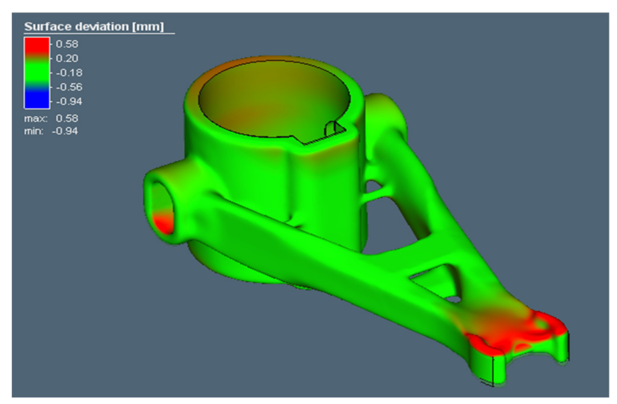
3.2. Simulation for Total Displacement in MSC Simufact

Performing a simulation in the MSC Simufact program involves eight steps. After importing the geometry, support elements are generated or imported. In the third step, the manufacturing parameters are defined, as shown in Table 2. By selecting the AM printer, the dimensions of the working environment are automatically set; then, the distance of the z axis direction is manually set. In the fourth step, a surface and voxel mesh are formed, as shown in Figure 10a. The surface mesh is set to 2 mm by default for each analysis. A surface mesh is the type of mesh that was transferred to the shifting thumb part after the voxel mesh. The voxel element size was set to 1 mm. The voxel mesh was then used to directly analyze the deformations (see Figure 10b). The main reason for creating the surface and voxel mesh was to make the part as close as possible to the actual shape. The fifth step in this software analyzes the results and shows a preview. In the sixth step, the results are graphically displayed and are subsequently used to calculate the pre-deformed model, as well as undergo any further analysis. The penultimate step consists of removing the supporting elements. In the last step, the part is cut from the build plate.

In this study, the layer height was set to 0.05 mm, and the inherent strains of ε_xx = −0.0036, ε_yy = −0.0036, and ε_zz = −0.03 were set to a uniform distribution. These values were determined via calibration with a reference structure for the equipment used. From the results of the simulation with the base plate, a total displacement in the range of 0.6–0.7 mm was obtained. The surface deformation deviation was 0.58 mm, and as with the ASS, the largest deformation on the nose of the component was evaluated, as shown in Figure 11.

3.3. Validation of the Results

The part was printed on the RENISHAW AM400 machine using stainless steel AISI 316L. After completing the printing process, excess powdered material was safely removed for recycling in future jobs. Then, the printed part was cut from the base plate, which was investigated to observe whether any deformation occurred on the printed part.

Testing was performed using digital image correlation (DIC). It can be observed in Figure 12 that the resulting deformation was slightly higher than the simulated deformation in Figure 9 and Figure 11. There are many factors that might play a role in such a difference. For instance, computational tools use different approaches and input parameters, which might result in different values. More obviously, the material properties that were employed in the simulation process using the ANSYS and MSC material libraries were the sources of the material properties assigned. The material properties of the printed part differed from the material properties available in the libraries. Further, the meshing of the bodies might have had a significant impact since the calculations were constrained to a limited number of elements. Moreover, heating due to slicing could be a factor in the significant additional deformation of the part.

Cutting from the base plate was realized using a saw blade, and the maximum displacement was measured as 1.137 mm. The base plate was taken into account as a reference, and the deviation from it was measured.

Verification by means of a 3D scanner was performed mainly to determine the degree of displacement after printing compared to the CAD model and to verify the functionality of the pre-programmed prestressed state.

In the first phase of scanning, when the part was still on the base plate, an average deviation of −0.210 mm was achieved, where the largest deviation was recorded on the nose of the part as −0.206 mm, which corresponds to the performed simulations (see Figure 13a). The second phase of the scan took place on already-cut parts that still had supporting elements on them. The achieved average deviation here was 0.229 mm. However, the activation of residual stresses was observed, and the part bent perpendicularly to the base plate and approached the desired shape when the deviation on the nose reached a value of −0.005 mm. The last scan was performed on components free of supporting elements. The removal of supports was done manually, which could have led to an error in the measurement; this error also appeared when the average deviation was measured as −0.541 mm. After removal of the supports, the required tolerance was reached in the part with the elongated holes (see Figure 13b), but the maximum deviation found on the nose was 1.326 mm. The value of the detected maximum deviation was, therefore, close to the result of the DIC measurement (taking into account the fact that maximal deflection is expected in the position where DIC results are not fully available; see Figure 12). That is also why we compare the numerical results with the 3D scanning results.

A comparison of the numerical results with the experimental results is provided in

Table 5. Numerical and experimental results of the maximal deflection of the part.

Numerical Method	Max. Value of Deflection
ANSYS Additive Suite	1.496 mm
MSC Simufact	0.580 mm
Experimental Method	Max. Value of Deflection
Digital image correlation	1.137 mm
3D scanner HandyScan	1.327 mm

. The lowest absolute difference between the numerical results and the experimental results in terms of maximal deflection was around 0.17 mm (11.4%) and was achieved using ANSYS Workbench.

4. Conclusions

This technical note presents a thorough workflow of 3D printing of metallic alloys to bridge the gap between designing and actual fabricating. Besides, it reveals the state-of-the-art knowledge in the field of stress analysis and simulations utilizing two commercial simulation software programs, AAS and MSC Simufact. A real component loaded with realistic forces was selected, which underwent topology optimization. Subsequently, simulations were performed in both programs. For both software programs, the default settings for material properties supplied by the manufacturer were used (these settings were not the same for both simulations). The part was also experimentally printed using the SLM method to verify the development of deformations during the part’s removal from the base plate. Thanks to the performed simulations and real verifications, several conclusions, which highlight the pros and cons of metallic 3D printing technology, were drawn:

• From a part designed for the traditional manufacturing method, utilization of topology optimization can reduce the volume of the part by up to 63%, while ensuring the equivalent strength. The 3D printing technology, subsequently, can be utilized to fabricate the complex optimized shape.
• Cost efficiency can be improved by minimizing the support structures when orienting the part on the base plate. However, as previously discussed, ac ompromise has to be made between the mechanical properties and the manufacturability of the printed parts. This factor, indeed, is most important for industrial and serial production.
• ANSYS simulation brings closer results to experiments considering deviation values.
• The two measurements realized by the different methods (DIC and 3D scanning) provided equivalent results for deflections, which contrasted with the numerical results. For more sufficient QC process, 3D scanning is recommended.
• When comparing the simulations with real measurements, a deviation of 0.17 mm was achieved. The nature of this difference was expected in the linear structural analysis. Significant residual stresses can lead to the yielding of the material. The stainless steel showed slight viscoplastic behavior, even at room temperature.
• To achieve higher precision in surface finishing or dimensioning below the deviation level presented in this study, extra surface treatment and machining must be carried out on the printed parts.
• The support elements generated in both pieces of software can be successfully utilized in place of supports generated in the slicer software.

Further studies will consider calibrating the software with the utilized machine, instead of setting the default printing values, with a hope of achieving better surface deviation prediction. Material properties of the in-used metal will be investigated so that more sophisticated numerical analysis can be performed. Moreover, multiple scanning strategies along with the use of multiple different print settings will be investigated.

References

1. Chen, Q.; Liang, X.; Hayduke, D.; Liu, J.; Cheng, L.; Oskin, J.; Whitmore, R.; To, A.C. An inherent strain based multiscale modeling framework for simulating part-scale residual deformation for direct metal laser sintering. Addit. Manuf. 2019, 28, 406–418. [Google Scholar] [CrossRef]
2. Ansari, J.; Nguyen, D.-S.; Park, H.S. Investigation of SLM Process in Terms of Temperature Distribution and Melting Pool Size: Modeling and Experimental Approaches. Materials 2019, 12, 1272. [Google Scholar] [CrossRef] [PubMed] [Green Version]
3. Hajnys, J.; Pagáč, M.; Měsíček, J.; Petru, J.; Król, M. Influence of scanning strategy parameters on residual stress in the SLM process according to the bridge curvature method for AISI 316L stainless steel. Materials 2020, 13, 1659. [Google Scholar] [CrossRef] [PubMed] [Green Version]
4. Lindgren, L. Computational Welding Mechanics; Woodhead: Cambridge, UK, 2007. [Google Scholar]
5. Chiumenti, M.; Cervera, M.; Salmi, A.; de Saracibar, C.A.; Dialami, N.; Matsui, K. Finite element modeling of multi-pass welding and shaped metal deposition processes. Comput. Methods Appl. Mech. Eng. 2010, 199, 2343–2359. [Google Scholar] [CrossRef]
6. Lundbäck, A.; Lindgren, L.-E. Modelling of metal deposition. Finite Elements Anal. Des. 2011, 47, 1169–1177. [Google Scholar] [CrossRef]
7. Hussein, A.; Hao, L.; Yan, C.; Everson, R.M. Finite element simulation of the temperature and stress fields in single layers built without-support in selective laser melting. Mater. Des. 2013, 52, 638–647. [Google Scholar] [CrossRef]
8. Zhang, D.; Cai, Q.; Liu, J.; Zhang, L.; Li, R. Select laser melting of W-Ni–Fe powders: Simulation and experimental study. Int. J. Adv. Manuf. Technol. 2010, 51, 649–658. [Google Scholar] [CrossRef]
9. Keller, N.; Ploshikhim, V. New method for fast predictions of residual stress and distortion of AM parts. In Annual International Solid Freeform Fabrication Symposium—An Additive Manufacturing Conference; The University of Texas: Austin, TX, USA, 2016; pp. 1229–1237. [Google Scholar]
10. Afazov, S.; Denmark, W.A.; Toralles, B.L.; Holloway, A.; Yaghi, A. Distortion prediction and compensation in selective laser melting. Addit. Manuf. 2017, 17, 15–22. [Google Scholar] [CrossRef]
11. Song, X.; Feih, S.; Zhai, W.; Sun, C.-N.; Li, F.; Maiti, R.; Wei, J.; Yang, Y.; Oancea, V.; Brandt, L.R.; et al. Advances in additive manufacturing process simulation: Residual stresses and distortion predictions in complex metallic components. Mater. Des. 2020, 193, 108779. [Google Scholar] [CrossRef]
12. Pástor, M.; Hagara, M.; Čarák, P. Residual stresses measurement around welds by optical methods. In Proceedings of the 58th International Scientific conference on Experimental Stress Analysis 2020, Luhacovice, Czech Republic, 3–6 June 2019; VSB-Technical University of Ostrava: Ostrava, Czech Republic, 2020; pp. 371–381, ISBN 978-80-248-4451-0. [Google Scholar]
13. Borralleras, P.; Segura, I.; Aranda, M.A.; Aguado, A. Influence of experimental procedure on d-spacing measurement by XRD of montmorillonite clay pastes containing PCE-based superplasticizer. Cem. Concr. Res. 2019, 116, 266–272. [Google Scholar] [CrossRef]
14. Mayer, T.; Brändle, G.; Schönenberger, A.; Eberlein, R. Simulation and validation of residual deformations in additive manu-facturing of metal parts. Heliyon 2020, 6, 1–13. [Google Scholar] [CrossRef]
15. Çelebi, A.; Appavuravther, E.Z. Analyzing the Effect of Voxel Mesh and Surface Mesh Application on Residual Stress by Simufact Additive Software. Düzce Üniversitesi Bilim ve Teknoloji Dergisi 2018, 6, 930–940. [Google Scholar] [CrossRef] [Green Version]
16. Bian, P.; Shi, J.; Liu, Y.; Xie, Y. Influence of laser power and scanning strategy on residual stress distribution in additively manufactured 316L steel. Opt. Laser Technol. 2020, 132, 106477. [Google Scholar] [CrossRef]
17. Training Manual 14TS210N; Kopřivnice: Kopřivnice, Czech Republic, 2011.
18. Sotola, M.; Stareczek, D.; Rybansky, D.; Prokop, J.; Marsalek, P. New Design Procedure of Transtibial ProsthesisBed Stump Using Topological Optimization Method. Symmetry 2020, 12, 1837. [Google Scholar] [CrossRef]
19. Jancar, L.; Pagac, M.; Mesicek, J.; Stefek, P. Design Procedure of a Topologically Optimized Scooter Frame Part. Symmetry 2020, 12, 755. [Google Scholar] [CrossRef]
20. Mesicek, J.; Pagac, M.; Petru, J.; Novak, P.; Hajnys, J.; Kutiova, K. Topological Optimization of the Formula Student Bell Crank. MM Sci. J. 2019, 2019, 2964–2968. [Google Scholar] [CrossRef]
21. Li, Y.; Zheng, T.; Yang, S.; Ren, Z. A methodology for topology optimization based on level set method and its application to piezoelectric energy harvester design. Int. J. Appl. Electromagn. Mech. 2019, 59, 79–85. [Google Scholar] [CrossRef]
22. Sigmund, O. Morphology-based black and white filters for topology optimization. Struct. Multidiscip. Optim. 2007, 33, 401–424. [Google Scholar] [CrossRef] [Green Version]
23. Bendsøe, M.P.; Sigmund, O. Topology Optimization: Theory, Method and Applications; Springer: Berlin/Heidelberg, Germany, 2007. [Google Scholar]
24. Sigmund, O.; Peterson, J. Numerical instabilities in topology optimization: A survey on procedures dealing with checker-boards, mesh-dependencies and local minima. Struct. Optim. 1998, 16, 68–75. [Google Scholar] [CrossRef]
25. Bruns, T.E.; Tortorelli, D.A. Topology optimization of non-linear elastic structures and compliant mechanisms. Comput. Methods Appl. Mech. Eng. 2001, 190, 3443–3459. [Google Scholar] [CrossRef]
26. ANSYS. ANSYS Workbench—ANSYS Help. 2020. Available online: https://ansyshelp.ansys.com/Account/Login?ReturnUrl=%2FViews%2FSecured%2Fcorp%2Fv195%2Fwb_sim%2Fds_topo_opt_level_set (accessed on 10 November 2020).
27. Hitzler, L.; Hirsch, J.; Heine, B.; Merkel, M.; Hall, W.; Öchsner, A. On the Anisotropic Mechanical Properties of Selective Laser-Melted Stainless Steel. Materials 2017, 10, 1136. [Google Scholar] [CrossRef] [PubMed] [Green Version]
Figure 1. Flowchart of the simulation model.
Applsci 11 01656 g001
Figure 2. Gear shift fork 14TS210 including the previous version of the shifting thumb [17].
Applsci 11 01656 g002
Figure 3. Original geometry of the main shifting thumb (a) and topologically smoothed shifting thumb (b).
Applsci 11 01656 g003
Figure 4. Boundary conditions applied to the model of the main shifting thumb (a) and resulting contours of von Mises stress (b).
Applsci 11 01656 g004
Figure 5. Resulting mesh and von Mises stress contours from the solid isotropic material with penalization (SIMP) method (a) and resulting mesh and von Mises stress contours from level-set method (b).
Applsci 11 01656 g005
Figure 6. Results of the simulations using a topologically smoothed shifting thumb in the form of von Mises stress contours: ANSYS Discovery Live (a) and ANSYS Workbench (b).
Applsci 11 01656 g006
Figure 7. 3D print position orientation using Autodesk Netfabb software (the gray arrows indicate the powder-laying direction).
Applsci 11 01656 g007
Figure 8. Additive manufacturing (AM) meshing for thermal analysis (a); thermal analysis results (b).
Applsci 11 01656 g008
Figure 9. Stand-alone structural analysis by the ASS.
Applsci 11 01656 g009
Figure 10. Voxel and surface mesh (a) and voxel mesh analysis (b).
Applsci 11 01656 g010
Figure 11. Stand-alone structural analysis using MSC Simufact.
Applsci 11 01656 g011
Figure 12. Maximum displacement on the left camera (a) and on the right camera (b).
Applsci 11 01656 g012
Figure 13. Representation of deviations detected by the 3D scanner: after printing (a) and after support removal (b).
Applsci 11 01656 g013