Article

Effects of Landscape Features on the Roadside Soil Heavy Metal Distribution in a Tropical Area in Southwest China

1
Research Institute of Forestry, Chinese Academy of Forestry, Beijing 100091, China
2
State Key Laboratory of Water Environment Simulation, School of Environment, Beijing Normal University, Beijing 100875, China
*
Author to whom correspondence should be addressed.
Appl. Sci. 2021, 11(4), 1408; https://doi.org/10.3390/app11041408
Submission received: 7 January 2021 / Revised: 25 January 2021 / Accepted: 26 January 2021 / Published: 4 February 2021
(This article belongs to the Special Issue Heavy Metals in the Environment – Causes and Consequences)

Abstract

:

Featured Application

Thus far, limited research has been carried out on a large scale that considers landscape characteristics, in-situ soil condition, or land cover. We aim to verify hitherto lacking evidence on the ability of vegetation characteristics and topographical factors to lessen pollutants in tropical regions in China.

Abstract

Soil heavy metals along roadsides pose a great threat to ecosystems while their spatial variations and influencing factors still remain unclear in some regions, especially in tropical areas with complex landscape characteristics. Our study was carried out to determine how the land use, vegetation characteristics, topographical factors and distance to the road affect the soil heavy metal distribution. Taking Jinghong county in Yunnan Province, Southwest China as a case, soil samples were collected at different distances off roads and canonical correspondence analysis (CCA) methods were used to determine the relative importance of different factors. Our results showed that heavy metal sources were obtained mainly from the road, based on the principle component analysis (PCA) identification. There were no obvious trends of soil quality index (SQI) with distance to the road in natural soils, while SQI nutrients and SQI metals in farmlands had a decreasing and increasing trend, respectively, which could both be expressed by logarithm models. However, soil properties showed little differences for road levels while they showed significant differences under land use types. The CCA further showed that heavy metal variations in natural soils were jointly affected by distance, plant coverage, relative elevation and soil properties in decreasing order.

1. Introduction

Roads, as an important linear landscape element, affect both abiotic and biotic ecosystems, especially the vegetation composition and soil properties along them [1,2]. In recent decades, studies on the ecological and environmental effects of road traffic have increased significantly [3,4,5,6]. In China, the development of road networks has been rapid with many high-level roads being constructed in recent years [7]. The negative effects, such as pollution, ecological damage, landscape fragmentation and hydrological connectivity interruption, are becoming more and more prominent and causing severe environmental, economic and even social issues, it is necessary to pay great attention to the road ecological protection [8].
Along with the extension and development of road networks, the contribution of road transportation to the emissions of atmospheric pollutants is regularly increasing [9]. The study of heavy metals and their risks has received much attention. The toxicity of heavy metals has been well investigated by researchers. Heavy metals are relatively serious pollutants not only because they are great potential hazards to human beings and other creatures [10], but they also accumulate in soils and are difficult to remove. Some heavy metals, including lead (Pb), cadmium (Cd), mercury (Hg), arsenic (As), and chromium (Cr), belong to priority control metals with high toxicities [11]. Heavy metals emitted from road vehicles into the atmosphere spread over wide regions, which could be called the “road effect zone” [12,13,14]. The road effect zone suffers from long-term accumulation of heavy metals, and these pollutants have an impact on the environment and nearby ecosystems. Some studies even focused on the relationships between cadmium pollution in view of tourism activities [15]. More studies have shown the contamination by these elements and the distribution of heavy metals in road dusts and soils [16,17,18]. Specifically, the effects mainly cause soil and plant environment disturbances [4]. Heavy metals can accumulate in topsoil from atmospheric deposition by sedimentation, impaction and interception, thus affecting the ecosystems directly or indirectly via changes to soil biogeochemistry and soil quality [6,19]. Although gasoline containing lead has been forbidden in China, the exhaust gas containing other heavy metals still shows significant effects on the soils.
Studies have shown that the distribution of heavy metals has many influencing factors, such as traffic level, wind direction, and topography [20]. In recent decades, the removal of pollutants by vegetation in the road effect zone has been of particular interest [21]. Pataki et al. (2011) stated that “the removal of atmospheric pollutants by vegetation is one of the most commonly cited ecosystem services”, yet it is one of the least supported empirically [22]. However, measurements on the uptake amount of air pollutants and rate of re-suspension by vegetation are not available [21]. Studies have verified that the understory vegetation plays an important role in regulating the nutrient fluxes, hydrology and micro climate of boreal forests and can accumulate considerable amounts of heavy metals and protect the soil from contamination [21]. Although Setälä et al. suggested that the urban area vegetation showed minor ability to remove air pollutants in northern climates with short growing seasons [21], the role of high vegetation canopy coverage for pollution mitigation in the tropical evergreen area needs further study. The concentration variations in roadside soils can provide valuable information in urban areas because such concentrations reflect the extent of the emissions from anthropogenic sources in most cases.
A spatial variability study is necessary for accurate prediction of soil contamination, as many uncertain results exist. As the total amount of heavy metals may be derived from anthropogenic and natural origins, it is difficult to determine a priori which of these two contributions will “decide” the variability [23]. Accordingly, the detection of contamination patterns with multivariate or multiple sample data involves determining which variables are of the most importance. Usually, the statistical methods of factor analysis (FA), principle component analysis (PCA), cluster analysis (CA), and correlation analysis have been widely used in evaluations of heavy metal pollution [24,25,26,27]. Previous studies often focused on a single heavy metal or influencing factor, and little research has been conducted on a larger scale, considering the landscape characteristics, in-situ soil conditions, or land cover. It is usual that the variation in soil nutrient status across landscapes is often analyzed using such techniques as regression and geostatistical analysis [28]. Other new multivariate methods are also recommended [29,30]. Recently, canonical correspondence analysis (CCA) has been widely applied in soil-environment research [31].
While there are many studies investigating roadside pollution in China, especially in urban areas, no studies thus far have demonstrated the spatial variability of heavy metals in tropical ecosystems [2,32,33,34]. The variation and accumulation of metallic pollutants along roads in this region require further study. In this paper, we aim to verify the hitherto lacking evidence on the ability of vegetation characteristics and topographical factors to decrease pollutants in tropical regions in China. For this purpose, the main highway that connects the Puer and Jinghong cities in Yunnan Province, Southwest China, was chosen. In the current study, special emphasis is placed on the relative ability of different factors. Based on previous studies, we assumed that soil pollutants decrease with increasing distance from the road [16,26], while the trends were not similar under different land uses. In addition, the pollutant accumulation and variations are related to the local landscape features [35,36,37,38]; however, the tropical areas in China need to be further explored. We considered the vegetation coverage and relative elevation of soil samples to the road as influencing factors, according to the field investigation. Thereby, our study uses multivariate methods to investigate the relationship between heavy metal contamination in roadside soils and its influencing factors. The objectives are to (1) reveal the spatial distribution of heavy metals near different roads; (2) use the CCA method to discern the relative importance of different influencing factors to immigrate heavy metal soil pollution.

2. Materials and Methods
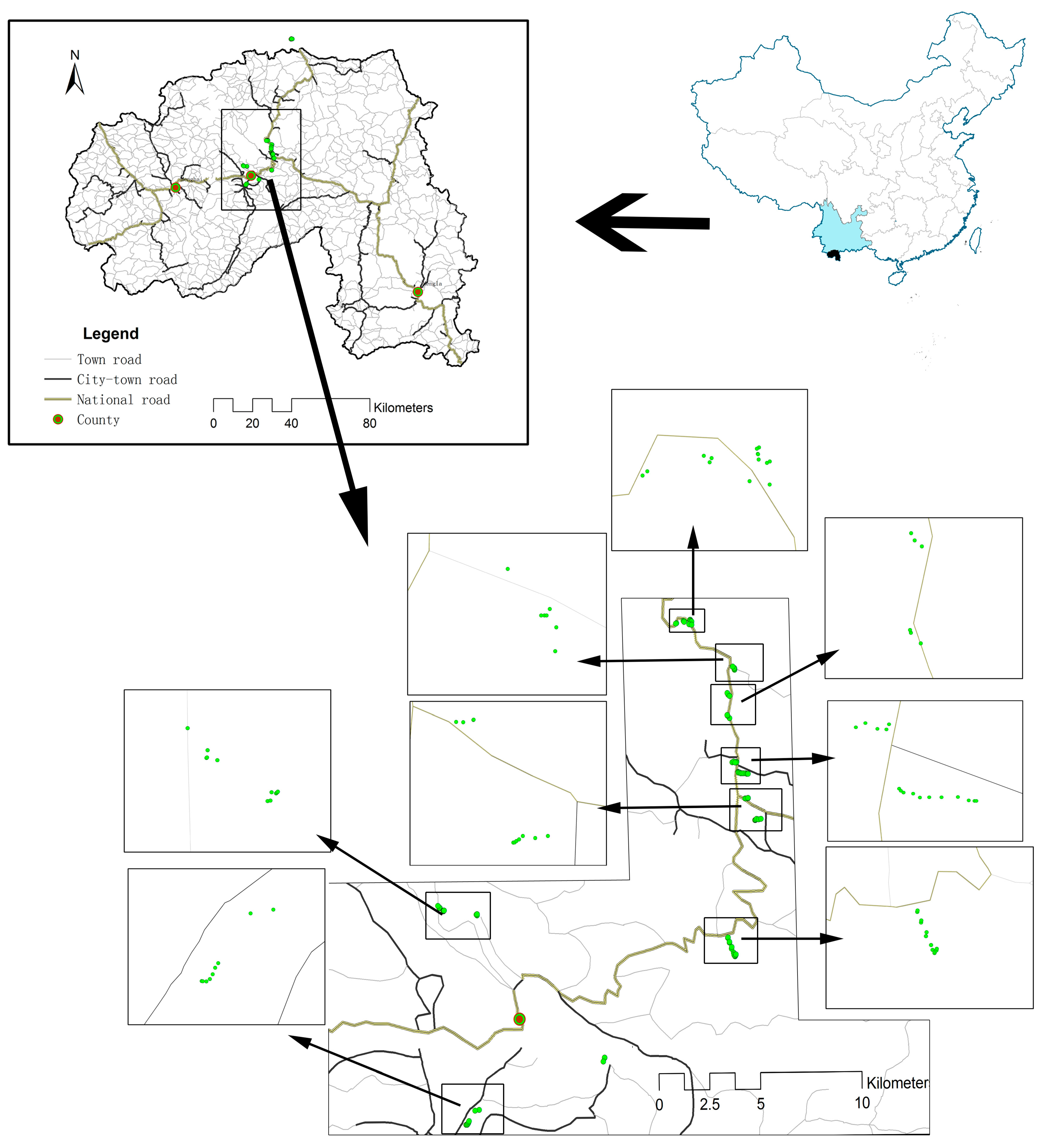
2.1. Study Area

The highway is located in the tropical regions in the southern part of Yunnan Province, which is approximately 50 km long connecting Puer and Jinghong cities for more than 35 years without a branch main road. In addition, two lower level roads were selected for comparison (Figure 1). All of the roads were located in the Lancang River valley (Upper Mekong River), an important eco-region for biodiversity and ecosystem conservation in China and in the world. Additionally, this region is famous in China for its diverse flora, fauna and beautiful landscape. It is estimated that approximately 5000 species of higher plants (16% of those in China) occur in this area of 19,200 km2 (0.2% of that of China). However, as the region is also an important ecological corridor of Yunnan Province toward Southeast Asia, it is vulnerable to scenarios, such as road development, thriving tourism and plantation. On both sides of the highway, agricultural lands and different land covers, including forest, shrubs, and grass, exist. In addition, the study road sections are far away from city and industrial sites, there are many topography variations and fewer villages, and atmospheric transportation of heavy metals from other sites is relatively low at these points. For the above reasons, the region provides a perfect background to study the regularity of soil heavy metal distribution near roads.

2.2. Basic Approach

To estimate the effect of road on soil, the transect line method was used for the soil sampling providing. Previous studies showed that the concentrations of heavy metals in roadside soils appear highest within 50 m from the road edge and reach the background values at 150 m [19,25,39]. Transect lines were taken as vertically as possible to the road, and the sampling distance was limited within 300 m off the road edge in the farmland and 200 m in the natural land area. Sampling intervals are small in areas within 50 m of the road and beyond 50 m, sampling distance is roughly 50 m apart. The soil type in this region is mainly red soil. The sample sites were chosen away from human constructions, such as gas station, service station, etc. The land use types included paddy field, grassland, dry land, natural forest, secondary forest, artificial forest and shrub land, and the total numbers of samples were 119, 10, 16, 30, 16, 18, 12, and 17 for each land use type, respectively.
The natural, secondary and artificial forests are mainly tropical rain, mixed broad-leaved and rubber plantation forests, respectively. Due to the landscape heterogeneity in the study region, the sample sizes for each land use type were different. At each site, a 10 × 10 m quadrate was set to investigate the vegetation community characteristics. For the soil sites, the relative elevation and distance from the road were recorded. Soil samples were obtained using cores (5 cm diameter) from three soil profiles at each site. The soil was sampled at a depth of approximately 0–20 cm, and the three replicate samples were homogenized. Then, the soil samples were air-dried and sieved for the determination of soil nutrients. The soil characteristics examined for the surface layer included pH, soil organic matter (SOM), total nitrogen (TN), available potassium (AK), available phosphorus (AP), total potassium (TK) and total phosphorus (TP) by colorimetry after wet digestion with H2SO4 and HClO4 [40]. The determination of TN was by the semi-micro Kjeldahl method. SOM was determined by the K2Cr2O7 titration method after digestion [41]. AP and AK were extracted with a 3% (NH4)2CO3 solution. After filtering, the filtrate was measured by inductively coupled plasma atomic absorption spectrometry (ICP/AES). TK was determined by atomic absorption spectrometry. The metals investigated were Pb, As, Cr, Zn, Cd, Cu, and Ni. Although China has been using unleaded fuel for years, a major reservoir of lead in roadside soils still remains because the Pb present on the roadside from historical environmental emissions is stable and mainly concentrated in the surface layers. Soil samples were digested in a sand bath using a mixture of 3:1:1 nitric acid:perchloric acid:hydrofluoric acid at 160 °C over 6 h until no more fumes were liberated and the color of the mixture turned pale-yellow to colorless. After that, samples were filtered through filter papers, and the volumes were adjusted to 25 mL using distilled water. Finally, concentrations of these metals were measured by inductively coupled plasma atomic absorption spectrometry (ICP/AES).

2.3. Statistical Analyses

A modified comparable soil quality index was developed to determine the effect of the road on soil quality associated with soil nutrients and soil heavy metals referring to the soil deterioration index [42,43]. It was computed on the assumption that the status of the individual soil properties was once the same as that of adjacent soils. The equation of SQI is expressed below:
S Q I = i = 1 n Q ( x i ) × 100 % / n
where xi is the value of soil properties selected for the soil quality; Q(xi) is the membership values of different soil properties; Q(xi) were calculated by the ascending and descending functions. Descending function was used for heavy metals as its higher contents often indicated soil quality degradation.
Q ( x i ) = ( x i j x i min ) / ( x i max x i min )  
Q ( x i ) = ( x i max x i j ) / ( x i max x i min )  
where xij is the values of soil properties; ximax and ximin are the maximum and minimum value of the i soil property in the same transect line. So, SQI indexes could be compared across all the transect lines at different locations.
In addition, multivariable statistic approaches were performed for influencing factor analysis. The PCA method was used to identify soil heavy metal sources. The paired-samples T test was used to compare the metal concentrations under different land uses and near different road levels. The Kaiser–Meyer–Olkin (KMO) and Bartlett’s sphericity tests were performed to examine the suitability of the data. One-way analysis of variance (ANOVA) procedures were used to compare the effects of different influencing factors. The ANOVA was conducted using the SAS program.
Finally, we used CCA for direct gradient analysis to identify the relative importance of different influencing factors of heavy metals for the natural soils. It has been suggested that CCA is the most feasible ordination method for performing direct gradient analysis. The software program Canoco 4.0 was used for data processing [44]. The data sets in our study contain i plots (i = 1 to n), k influencing variables (k = 1 to m) and q soil heavy metal attributes. We selected the pH, TP and TK as the soil property indicators significantly related to heavy metals, plant layer coverage as the land cover indicator, relative elevation as the topography indicator, and distance off road as the horizontal influencing indicator. These influencing factors were set as environmental independent variables and the soil heavy metals as dependent variables. Let Y be the data matrix of the variables, an n × k matrix of variables data (119 × 6 matrix), E be the matrix of soil heavy metal attributes, and an n × p matrix of dependent variables data (119 × 7 matrix) be the plots of heavy metal attributes. Thus, yik, an element of Y, is the value of variable k at plot i, and eij, an element of E, is the value of soil heavy metal attribute j at plot i. The following steps are performed within each CCA iteration [31]:
(1) Choose arbitrary, but unequal, initial plot scores (xi).
(2) Calculate soil series scores (uk) by weighted averaging of the plot scores with λ = 1 (where λ is eigenvalue; see step 7). This is a transition formula that links Gaussian ordination to CCA [45]:
λ u k = i = 1 n y i k x i / y o k
where yok is the variable or soil series total:
y o k = i = 1 n y i k
(3) Calculate new plot scores by weighted averaging of the soil series scores:
x i * = i = 1 n y i k u k / y i o
where yio is the sites or plots total:
y i o = i = 1 m y i k
(4) Obtain regression coefficients by weighted multiple regression analysis of the plot scores on soil heavy metal variables:
b = ( E D E ) 1 E D x *
where b is a column vector of canonical coefficients, i.e., b = (bo, b1, …, bp)′, x* is a column vector of the new plot scores, i.e., x* = (x*1, …, x*n)′, E is the soil heavy metal attribute data set and D is a diagonal n × n matrix with yio.
(5) Calculate new plot scores from the regression coefficients:
X = E b
where x is a column vector: x = (x1, ...., xn)′.
(6) Center and standardize the plot scores [46]:
Step 6-1: Calculate the centroid, z, of the plot scores (xi):
z = i = 1 n y i o x / y o o
Step 6-2: Calculate the dispersion of the plot scores:
S 2 = i = 1 n y i o ( x z ) 2 / y o o
where
y o o = i = 1 m y i o
Step 6-3: Calculate xi,new as below:
x i , n e w   = ( x i , o l d z ) / s
Step 6-4: Denote the plot scores of the previous axis by fi and the trial scores of the present axis by xi.
Step 6-5:
Calculate:
v = i = 1 n y i o x i f i / y o o
Step 6-6: Calculate xi,new = xi,old − vfi. These are the new trial plot scores, which are now orthogonal to those of the previous axes.
Step 6-7: Repeat Steps (6-4) to (6-7) for all previous axes.
(7) Repeat all steps from Step 2, using the plot scores from Step 6. Stop when the new plot scores do not differ within a prescribed tolerance level of 10−13 [47] from the plot scores of the previous iteration. The sum of the squares of the plot scores at convergence equals the eigenvalue (λ).
(8) Obtaining additional axes requires an additional step after Step 5 to make the trial scores uncorrelated with the previous axes [48].

3. Results

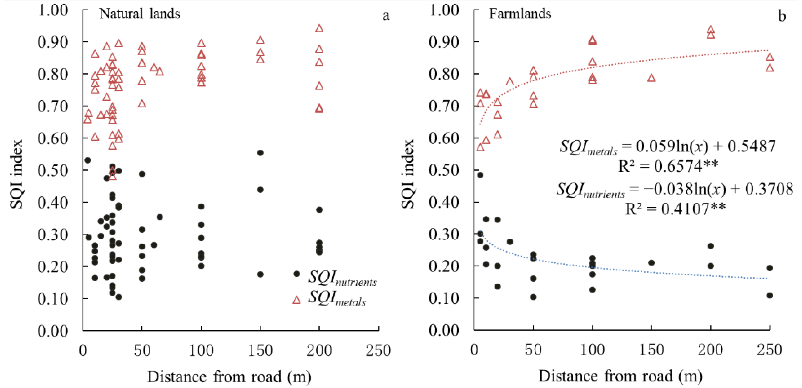
3.1. SQI Variations with Distances to Roads

The calculated integrated SQI reflects the relative soil quality degree of different soil points away from the roads. Using Equations (1) and (2), the membership value Q(xi) of each soil quality factor was calculated and the SQI for soil nutrients and soil heavy metals (SQInutrients and SQImetals) could be compared. The higher values of SQI mean higher soil fertility and less soil contamination.
Figure 2 shows the trends of SQI index with distance to roads. We classified the points to the natural lands and farmlands. It is very clear that the SQI values varied greatly in the natural soils regardless of soil nutrients or soil heavy metals (Figure 2a). No obvious trends were found for the points in natural soils. However, in farm dry lands, it is clear that the SQInutrients had a general decreasing trend and SQImetals had an increasing trend. Both changing trends with the distances in farmlands could be fitted by logarithm models with significant levels (p < 0.01) (Figure 2b).

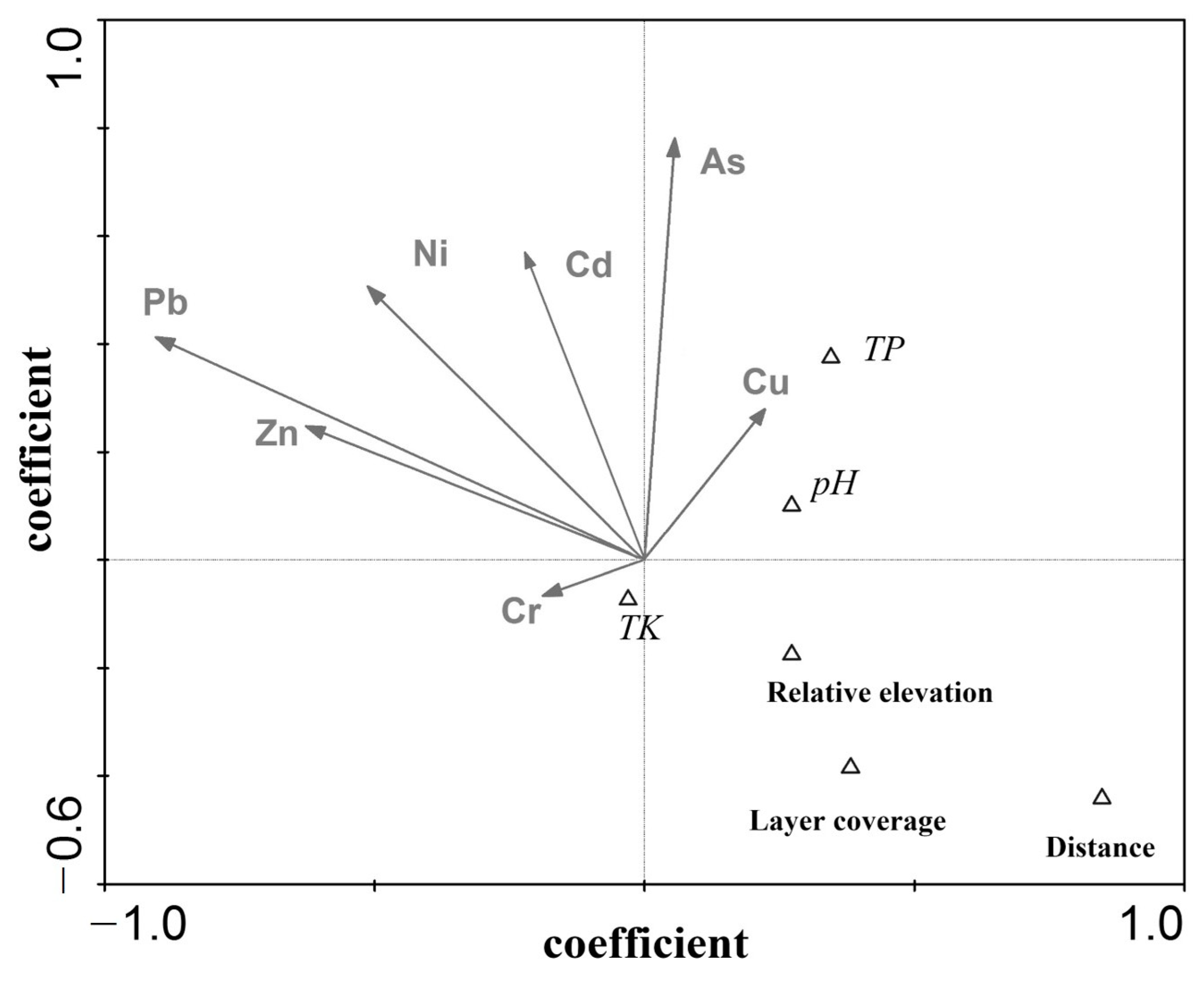
3.2. Source Identification of Pollutants

The relationship between different heavy metals in soil can also indicate whether the source is the same. Using Spearman’s correlation analysis, we found that there were significant relationships between different heavy metals implying that the pollutants may be homologous from the road. Furthermore, we used the PCA method to identify the correlations among the original variables in a data set. The results of the PCA analysis showed that heavy metal concentrations along the roads could be represented by two main components, which accounted for 82.48% of the total variance (Table 1). The first component, with a variance of 65.03%, was highly correlated with As, Cd, Cu, Pb and Zn. This component could be identified as an “anthropogenic factor” and might originate from a common source due to road traffic [49]. The second component accounted for 17.45% of the total variance with high loadings on Cr and Ni. We can label this component the “natural factor”, which might also be controlled by the parent rock composition. It could be deduced that the pollutants mainly originate from road traffic [50].

3.3. Influencing Factors on Soil Properties Variability

3.3.1. Effects of Different Road Levels

As shown in Table 2, the soil characteristics of pH, TK, TP, AK, TN, SOM and AP varied near different road levels. Road level I, II and III indicate national road, county road (road between county cities ) and town road (county city–town road). However, only SOM, TN and TK showed significant differences depending on road level. As the land use distribution could be affected by road networks, the variations in soil properties near the road imply an indirect effect of road levels on nutrient distribution. Similar results of weak significance were found for different heavy metals, as shown in Table 3. Although the lowest levels of As, Zn, Pb, Cu, Cd, and Ni can be found under road level III, the F value indicated no significance for the three road levels.

3.3.2. Effects of Land Uses

The physical and chemical properties of soil have close relationships with plant growth, soil microorganisms and soil enzyme activity, and some properties, such as pH and SOM, can affect the transfer, adsorption and availability of heavy metals. Thus, we first discuss the differences in heavy metals under different land use types. ANOVA was used to compare the differences among the seven land uses. Table 4 shows the comparison among the different land uses. It shows there are statistically significant differences in pH, SOM, TN, TP and TK content among land use types (p < 0.05). For TN and SOM, the natural forest was higher, followed by the secondary forest. The secondary forest also had higher AP and AK content. A close observation reveals that artificial forest and farmland had lower soil nutrient levels.
Table 5 indicates the heavy metals under different land uses. The F value by the ANOVA method showed that significant differences exist in most heavy metals, except for As, Cd and Ni. It is evident that the trends are similar among the different land uses. Grassland had the highest levels of Pb, Zn, Ni, As, Cr, and Cu, while the secondary and natural forests had the lower levels.

3.3.3. Importance of Influencing Factors in Natural Soils

To further investigate the importance of influencing factors and the relationship between soil properties and soil heavy metals, we used CCA to quantify the relative importance. The CCA method screened out the importance of those factors. The results of the influencing factor and heavy metal relationship are shown in Figure 3. The CCA figure can be displayed in an ordination diagram in which scores for the influencing factors are indicated as arrows and scores of soil properties represented by points. The CCA showed that the cumulative percentage variance of the first and second axis were 75% and 92%. Monte Carlo permutation tests confirmed the overall significance of the canonical ordination (p = 0.01) and the significance of the first axes (p = 0.02). This result confirmed that both axes jointly represented soil heavy metal distribution, as determined from the CCA ordination. From the figure, we can derive that distance is the most influencing factor in this region. Layer coverage, topography and soil intrinsic properties also impact soil heavy metals. The order is distance > layer coverage > relative elevation > soil properties (pH, TP, and TK).

4. Discussion

4.1. Heavy Metal Variations Associated with Roads

In general, heavy pollutant levels will show exponential decay with distance from the road. In our study, SQI values for natural lands and farmlands were separately calculated to elucidate the trends. We derived the SQI values based on the soil deterioration index. Although different weights could be added for different soil factors to get a comprehensive SQI, studies also showed that soil deterioration index method with direct difference was also a simple and effective way to determine the changes of soil quality [13].
Many studies have determined that the highest concentrations of heavy metals in soil will be found within 20–30 m from the road [51]. In our study, SQI kept stable after about 50m away the road. It is consistent with the other study results. In addition, from the results of Figure 2, it could be concluded that more influencing factors other than distance resulted in the complex spatial distribution of soil heavy metals in the natural soils.
Our results verified that there are many uncertainties to reveal the heavy metal variations within different road buffers. Further research needs to be undertaken in different habitat types and climatic regions in association with different road types and pollutants [15].
Previous studies usually used the correlation and PCA method to identify the pollution sources [2,51]. In our results, the PCA method was efficient and screened out the two components. The results distinguished that As, Cd, Cu, Pb and Zn originated from a common source due to road traffic [51]. A similar study in Brazil showed that road-deposited sediments accumulate a variety of toxic substances, and the soils were moderately polluted for Cu and slighted polluted for Zn and Pb [2]. Studies verified that Zn, Cu, Pb, and Cd are likely due to tire material degrading and traffic volume causing greater brake pads. Of the soil heavy metals investigated in this study, Cu, Zn and Ni are essential micronutrients for plants but become toxic for plants at higher concentrations [52,53]. Pb and Cd are non-essential for plants and may be toxic or lethal at small amounts. Thus, road pollution may also cause harmful damage to neighboring plant communities [54].

4.2. Quantification of the Influencing Factors of Heavy Metals and Management Implications

Some studies showed that the variability of soil heavy metals along the road was influenced by certain factors, such as climate, soil types, and parent soil materials [4]. In fact, these factors influence the soil heavy metal variability on a large scale. On a small scale, in the vicinity of the roads, a number of factors aside from traffic density will explain pollutant concentration away from the roadside [55]. In the tropical area, the land use types, topography, and land coverage may affect the distribution, and our analysis verified the phenomenon in the study area [56].
Spatial variation assessment helps to lessen the heavy metal pollution in practical way. In the tropical area, studies even showed that tropical climate can influence the toxic heavy metal pollutant course of road-deposited sediments [2]. Our results verified that land cover alongside the road had great influence on heavy metal deposition. In the study area, heavy metal concentrations were highest in grassland while much lower on the farmland. The reason is that transfer is fast on the farmland due to frequent tillage disturbance. In addition, as the secondary and natural forests had higher layer coverage and heavy metal diffuse was limited to a small extent, the content was relatively low. Previous studies also showed that trees can efficiently filter pollutant particles from the air [36]. This result is consistent with former studies [6,57]. It is true that cultivation can disturb the land cover or soil layers, which results in an increase in temperature and then the higher decomposition rate of SOM [58].
Effective pollution control management measurements such as road sweeping and traffic controlling measures, are important to lessen soil pollution [39]. The heavy metal pattern along the road and the influencing factors should be considered when the environmental protection and planning along the roads are conducted in the future [59]. In this area, shrub lands have the largest layer coverage and could act as a buffer to mitigate the roadside soil pollution. So, natural vegetation conservation might be the best management practice to minimize soil heavy metal accumulation.

5. Conclusions

Our study demonstrated that the SQI index could indicate the comprehensive effects of road pollution on surrounding ecosystems. The SQI trends expressed by the logarithm models with distance to road were different for soil nutrients and heavy metals in farmlands. Road levels had little effect on soil pollution while soil heavy metals showed significant differences under different land use types. However, there existed more uncertainty for the heavy metal contents in natural soils due to the vegetation and other topographical factors. In the natural lands, grassland had the highest levels of Pb, Zn, Ni, As, Cr, and Cu, while the secondary and natural forests had the lower levels. When the metal data sets were studied using CCA to ascertain whether the importance of different influencing factors can be sought, it was found that the joint effect of distance, topography, and plant community coverage can largely explain the natural soil contamination variability. The CCA results showed that the importance of influencing factors in the study region is distance > layer coverage > relative elevation > soil properties. Our study was conducted to reveal heavy metal pollution and its influencing factors in a certain region. Within the scope of our results, it is recommended to conduct further studies on roadside atmospheric transportation modeling.

Author Contributions

Conceptualization, Y.D. and S.L.; methodology, S.L.; software, Y.S.; formal analysis, Y.L.; investigation, S.L.; data curation, S.L.; writing—original draft preparation, Y.D.; writing—review and editing, S.L.; visualization, F.W.; supervision, S.L.; project administra-tion, S.L. All authors have read and agreed to the published version of the manuscript.

Funding

The work was supported by the National Natural Sciences Foundation of China (No. 41571173) and the second scientific expedition to the Qinghai-Tibet Plateau (No. 2019QZKK0405-05) and Nonprofit Environment Protection Specific Project of China (No. 201209029).

Institutional Review Board Statement

Not applicable.

Informed Consent Statement

Not applicable.

Data Availability Statement

The data presented in this study are available on request from the corresponding author. The data are not publicly available due to privacy restrictions.

Conflicts of Interest

The authors declare no conflict of interest.

References

  1. Mullerova, J.; Vitkova, M.; Vitek, O. The impacts of road and walking trails upon adjacent vegetation: Effects of road building materials on species composition in a nutrient poor environment. Sci. Total Environ. 2011, 409, 3839–3849. [Google Scholar] [CrossRef] [PubMed]
  2. Dos Santos, P.R.S.; Fernandes, G.J.T.; Moraes, E.P.; Moreira, L.F.F. Tropical climate effect on the toxic heavy metal pollutant course of road-deposited sediments. Environ. Pollut. 2019, 251, 766–772. [Google Scholar] [CrossRef] [PubMed]
  3. Forman, R.T.T. Estimate of the area affected ecologically by the road system in the United States. Conserv. Biol. 2000, 14, 31–35. [Google Scholar] [CrossRef]
  4. Lee, M.A.; Davies, L.; Power, S.A. Effects of roads on adjacent plant community composition and ecosystem function: An example from three calcareous ecosystems. Environ. Pollut. 2012, 163, 273–280. [Google Scholar] [CrossRef] [PubMed]
  5. Truscott, A.M.; Palmer, S.C.F.; McGowan, G.M.; Cape, J.N.; Smart, S. Vegetation composition of roadside verges in Scotland: The effects of nitrogen deposition, disturbance and management. Environ. Pollut. 2005, 136, 109–118. [Google Scholar] [CrossRef] [PubMed]
  6. Hong, N.; Guan, Y.J.; Yang, B.; Zhong, J.; Zhu, P.F.; Ok, Y.S.; Hou, D.Y.; Tsang, D.C.W.; Guan, Y.T.; Liu, A. Quantitative source tracking of heavy metals contained in urban road deposited sediments. J. Hazard. Mater. 2020, 393, 8. [Google Scholar] [CrossRef] [PubMed]
  7. Liu, S.L.; Cui, B.S.; Dong, S.K.; Yang, Z.F.; Yang, M.; Holt, K. Evaluating the influence of road networks on landscape and regional ecological risk-A case study in Lancang River Valley of Southwest China. Ecol. Eng. 2008, 34, 91–99. [Google Scholar] [CrossRef]
  8. Zhang, M.; Liu, X.; Ding, Y. Assessing the influence of urban transportation infrastructure construction on haze pollution in China: A case study of Beijing-Tianjin-Hebei region. Environ. Impact Asses. 2021, 87, 106547. [Google Scholar] [CrossRef]
  9. Shi, G.T.; Chen, Z.L.; Xu, S.Y.; Zhang, J.; Wang, L.; Bi, C.J.; Teng, J.Y. Potentially toxic metal contamination of urban soils and roadside dust in Shanghai, China. Environ. Pollut. 2008, 156, 251–260. [Google Scholar] [CrossRef]
  10. Han, R.R.; Zhou, B.H.; Huang, Y.Y.; Lu, X.H.; Li, S.; Li, N. Bibliometric overview of research trends on heavy metal health risks and impacts in 1989-2018. J. Clean. Prod. 2020, 276, 10. [Google Scholar] [CrossRef]
  11. Alsanad, A.; Alolayan, M. Heavy metals in road-deposited sediments and pollution indices for different land activities. Environ. Nanotechnol. Monit. Manag. 2020, 14, 100374. [Google Scholar] [CrossRef]
  12. Hilton, F.G.H.; Levinson, A. Factoring the environmental kuznets curve: Evidence from automotive lead emissions. J. Environ. Econ. Manag. 1998, 35, 126–141. [Google Scholar] [CrossRef] [Green Version]
  13. Turer, D.G.; Maynard, B.J. Heavy metal contamination in highway soils. Comparison of Corpus Christi, Texas and Cincinnati, Ohio shows organic matter is key to mobility. Clean Technol. Envir. 2003, 4, 235–245. [Google Scholar] [CrossRef]
  14. Zhang, H.; Ma, D.; Xie, Q.; Chen, X. An approach to studying heavy metal pollution caused by modern city development in Nanjing, China. Environ. Geol. 1999, 38, 223–228. [Google Scholar] [CrossRef]
  15. Mikhailenko, A.V.; Ruban, D.A.; Ermolaev, V.A.; van Loon, A.J. Cadmium Pollution in the Tourism Environment: A Literature Review. Geosciences 2020, 10, 19. [Google Scholar] [CrossRef]
  16. Neher, D.A.; Asmussen, D.; Lovell, S.T. Roads in northern hardwood forests affect adjacent plant communities and soil chemistry in proportion to the maintained roadside area. Sci. Total Environ. 2013, 449, 320–327. [Google Scholar] [CrossRef]
  17. Wang, Z.L.; He, J.; Biao, Z.Y.; Wang, Z.S.; Wang, L.X.; Liu, H.M.; Lv, C.W.; Jiang, C. The distribution characteristics of heavy metals pollutants in soil-plant system along highway. J. Nanjing For. Univ. 2006, 30, 15–20. [Google Scholar]
  18. Zhu, J.J.; Cui, B.S.; Yang, Z.F.; Dong, S.K.; Yao, H.R. Spatial distribution and variability of heavy metals contents in the topsoil along roadside in the Longitudinal Range-Gorge Region in Yunnan Province. Acta Ecol. Sin. 2006, 26, 146–153. [Google Scholar]
  19. Wei, B.G.; Jiang, F.Q.; Li, X.M.; Mu, S.Y. Spatial distribution and contamination assessment of heavy metals in urban road dusts from Urumqi, NW China. Microchem. J. 2009, 93, 147–152. [Google Scholar] [CrossRef]
  20. Zhang, H.; Ma, D.S. An approach to the characteristics of heavy metal phases as well as the capacity of desorption and adsorption in soils about heavy metal pollution formed by highway. Environ. Chem. 1998, 17, 564–568. [Google Scholar]
  21. Setala, H.; Viippola, V.; Rantalainen, A.L.; Pennanen, A.; Yli-Pelkonen, V. Does urban vegetation mitigate air pollution in northern conditions? Environ. Pollut. 2013, 183, 104–112. [Google Scholar] [CrossRef]
  22. Pataki, D.E.; Carreiro, M.M.; Cherrier, J.; Grulke, N.E.; Jennings, V.; Pincetl, S.; Pouyat, R.V.; Whitlow, T.H.; Zipperer, W.C. Coupling biogeochemical cycles in urban environments: Ecosystem services, green solutions, and misconceptions. Front. Ecol. Environ. 2011, 9, 27–36. [Google Scholar] [CrossRef]
  23. Carlosena, A.; Andrade, J.M.; Prada, D. Searching for heavy metals grouping roadside soils as a function of motorized traffic influence. Talanta 1998, 47, 753–767. [Google Scholar] [CrossRef]
  24. Abrahim, G.M.S.; Parker, R.J. Assessment of heavy metal enrichment factors and the degree of contamination in marine sediments from Tamaki Estuary, Auckland, New Zealand. Environ. Monit. Assess. 2008, 136, 227–238. [Google Scholar] [CrossRef] [PubMed]
  25. Carrero, J.A.; Arrizabalaga, I.; Bustamante, J.; Goienaga, N.; Arana, G.; Madariaga, J.M. Diagnosing the traffic impact on roadside soils through a multianalytical data analysis of the concentration profiles of traffic-related elements. Sci. Total Environ. 2013, 458, 427–434. [Google Scholar] [CrossRef] [PubMed]
  26. Han, D.C.; Zhang, X.O.; Tomar, V.V.S.; Li, Q.; Wen, D.Z.; Liang, W.J. Effects of heavy metal pollution of highway origin on soil nematode guilds in North Shenyang, China. J. Environ. Sci. 2009, 21, 193–198. [Google Scholar] [CrossRef]
  27. Zhao, Q.H.; Liu, S.L.; Deng, L.; Yang, Z.F.; Dong, S.K.; Wang, C.; Zhang, Z.L. Spatio-temporal variation of heavy metals in fresh water after dam construction: A case study of the Manwan Reservoir, Lancang River. Environ. Monit. Assess. 2012, 184, 4253–4266. [Google Scholar] [CrossRef] [PubMed]
  28. Western, A.W.; Bloschl, G.; Grayson, R.B. Geostatistical characterisation of soil moisture patterns in the Tarrawarra a catchment. J. Hydrol. 1998, 205, 20–37. [Google Scholar] [CrossRef]
  29. Liu, S.L.; Guo, X.D.; Fu, B.J.; Lian, G.; Wang, J. The effect of environmental variables on soil characteristics at different scales in the transition zone of the Loess Plateau in China. Soil Use Manag. 2007, 23, 92–99. [Google Scholar] [CrossRef]
  30. Qiu, Y.; Fu, B.J.; Wang, J.; Chen, L.D. Spatial variability of soil moisture content and its relation to environmental indices in a semi-arid gully catchment of the Loess Plateau, China. J. Arid. Environ. 2001, 49, 723–750. [Google Scholar] [CrossRef] [Green Version]
  31. Bodaghabadi, M.B.; Salehi, M.H.; Martinez-Casasnovas, J.A.; Mohammadi, J.; Toomanian, N.; Borujeni, I.E. Using Canonical Correspondence Analysis (CCA) to identify the most important DEM attributes for digital soil mapping applications. Catena 2011, 86, 66–74. [Google Scholar] [CrossRef]
  32. Li, Z.Y.; Ma, Z.W.; van der Kuijp, T.J.; Yuan, Z.W.; Huang, L. A review of soil heavy metal pollution from mines in China: Pollution and health risk assessment. Sci. Total Environ. 2014, 468, 843–853. [Google Scholar] [CrossRef]
  33. Liu, E.F.; Yan, T.; Birch, G.; Zhu, Y.X. Pollution and health risk of potentially toxic metals in urban road dust in Nanjing, a mega-city of China. Sci. Total Environ. 2014, 476, 522–531. [Google Scholar] [CrossRef]
  34. Wei, B.G.; Yang, L.S. A review of heavy metal contaminations in urban soils, urban road dusts and agricultural soils from China. Microchem. J. 2010, 94, 99–107. [Google Scholar] [CrossRef]
  35. MacKinnon, G.; MacKenzie, A.B.; Cook, G.T.; Pulford, I.D.; Duncan, H.J.; Scott, E.M. Spatial and temporal variations in Pb concentrations and isotopic composition in road dust, farmland soil and vegetation in proximity to roads since cessation of use of leaded petrol in the UK. Sci. Total Environ. 2011, 409, 5010–5019. [Google Scholar] [CrossRef] [Green Version]
  36. Salemaa, M.; Vanha-Majamaa, I.; Derome, J. Understorey vegetation along a heavy-metal pollution gradient in SW Finland. Environ. Pollut. 2001, 112, 339–350. [Google Scholar] [CrossRef]
  37. Steffens, J.T.; Wang, Y.J.; Zhang, K.M. Exploration of effects of a vegetation barrier on particle size distributions in a near-road environment. Atmos. Environ. 2012, 50, 120–128. [Google Scholar] [CrossRef]
  38. Wannaz, E.D.; Carreras, H.A.; Perez, C.A.; Pignata, M.L. Assessment of heavy metal accumulation in two species of Tillandsia in relation to atmospheric emission sources in Argentina. Sci. Total Environ. 2006, 361, 267–278. [Google Scholar] [CrossRef]
  39. Li, F.R.; Kang, L.F.; Gao, X.Q.; Hua, W.; Yang, F.W.; Hei, W.L. Traffic-related heavy metal accumulation in soils and plants in northwest China. Soil. Sediment. Contam. 2007, 16, 473–484. [Google Scholar] [CrossRef]
  40. Parkinson, J.A.; Allen, S.E. A wet oxidation procedure suitable for the determination of nitrogen and mineral nutrients in biological material. Commun. Soil Sci. Plan. 1975, 6, 1–11. [Google Scholar] [CrossRef]
  41. Nelson, D.W.; Sommers, L.E. A rapid and accurate method for estimating organic carbon in soil. Proc. Indiana Acad. Sci. 1975, 84, 456–462. [Google Scholar]
  42. Adejuwon, J.O.; Ekanade, O. A comparison of soil properties under different landuse types in a part of the Nigerian cocoa belt. Catena 1988, 15, 319–331. [Google Scholar] [CrossRef]
  43. Fu, B.J.; Liu, S.L.; Lu, Y.H.; Chen, L.D.; Ma, K.M.; Liu, G.H. Comparing the soil quality changes of different land uses determined by two quantitative methods. J. Environ. Sci. 2003, 15, 167–172. [Google Scholar]
  44. Biometry, C.F. Canoco for Windows 4.0; Centre for Biometry: Wageningen, The Netherlands, 1998. [Google Scholar]
  45. Terbraak, C.J.F. Correspondence-analysis of Incidence and bundance data: Properties in terms of a unimodal response model. Biometrics 1985, 41, 859–873. [Google Scholar] [CrossRef]
  46. Falero, E.M. Data analysis in community and landscape ecology: R.H.G. Jongman, C.J.F. ter Braak and O.F.R. van Tongeren, Pudoc, Wageningen, The Netherlands, 1987 (ISBN 90-220-0908-4). 208 pp. Price Dfl. 85.00/$42.50. Landscape Urban. Plan. 1989, 17, 371–372. [Google Scholar] [CrossRef]
  47. Oksanen, J.; Minchin, P.R. Instability of ordination results under changes in input data order: Explanations and remedies. J. Veg. Sci. 1997, 8, 447–454. [Google Scholar] [CrossRef]
  48. Odeh, I.O.A.; Chittleborough, D.J.; McBratney, A.B. Elucidation of soil landform interrelationships by canonical ordination analysis. Geoderma 1991, 49, 1–32. [Google Scholar] [CrossRef]
  49. Liu, S.L.; Wang, C.; Yang, J.J.; Zhao, Q.H. Assessing the heavy metal contamination of soils in the water-level fluctuation zone upstream and downstream of the Manwan Dam, Lancang River. J. Soils Sediments 2014, 14, 1147–1157. [Google Scholar] [CrossRef] [Green Version]
  50. Ozaki, H.; Watanabe, I.; Kuno, K. As, Sb and Hg distribution and pollution sources in the roadside soil and dust around Kamikochi, Chubu Sangaku National Park, Japan. Geochem. J. 2004, 38, 473–484. [Google Scholar] [CrossRef]
  51. Sofowote, U.M.; Di Federico, L.M.; Healy, R.M.; Debosz, J.; Su, Y.S.; Wang, J.; Munoz, A. Heavy metals in the near-road environment: Results of semi-continuous monitoring of ambient particulate matter in the greater Toronto and Hamilton area. Atmos. Environ.-X 2019, 1, 11. [Google Scholar] [CrossRef]
  52. Marschner, H. Mineral Nutrition of Higher Plants; Academic Press: London, UK, 1995; p. 889. [Google Scholar]
  53. Ouyang, J.F.; Liu, Z.R.; Zhang, L.; Wang, Y.; Zhou, L.M. Analysis of influencing factors of heavy metals pollution in farmland-rice system around a uranium tailings dam. Process. Saf. Environ. Protect. 2020, 139, 124–132. [Google Scholar] [CrossRef]
  54. Wahab, M.I.A.; Abd Razak, W.M.A.; Sahani, M.; Khan, M.F. Characteristics and health effect of heavy metals on non-exhaust road dusts in Kuala Lumpur. Sci. Total Environ. 2020, 703, 11. [Google Scholar] [CrossRef] [PubMed]
  55. Zhang, J.; Wang, X.; Zhu, Y.; Huang, Z.; Yu, Z.; Bai, Y.; Fan, G.; Wang, P.; Chen, H.; Su, Y.; et al. The influence of heavy metals in road dust on the surface runoff quality: Kinetic, isotherm, and sequential extraction investigations. Ecotox. Environ. Safe. 2019, 176, 270–278. [Google Scholar] [CrossRef] [PubMed]
  56. Jeong, H.; Choi, J.Y.; Lee, J.; Lim, J.; Ra, K. Heavy metal pollution by road-deposited sediments and its contribution to total suspended solids in rainfall runoff from intensive industrial areas. Environ. Pollut. 2020, 265, 115028. [Google Scholar] [CrossRef]
  57. Liu, S.L.; Fu, B.J.; Lu, Y.H.; Chen, L.D. Effects of reforestation and deforestation on soil properties in humid mountainous areas: A case study in Wolong Nature Reserve, Sichuan province, China. Soil Use Manage. 2002, 18, 376–380. [Google Scholar] [CrossRef]
  58. Barber, R.G. Soil degradation in the tropical lowlands of Santa Cruz, Eastern Bolivia. Land Degrad. Rehabil. 1995, 6, 95–107. [Google Scholar] [CrossRef]
  59. Lin, Y.; Wu, M.; Fang, F.; Wu, J.; Ma, K. Characteristics and influencing factors of heavy metal pollution in surface dust from driving schools of Wuhu, China. Atmos. Pollut. Res. 2020. [Google Scholar] [CrossRef]
Figure 1. Location of the study region and sampling transects.
Applsci 11 01408 g001
Figure 2. The changes of SQI index for soil nutrients and heavy metals with distance to road in natural lands and farmlands. (a): SQI index in the natural lands; (b): SQI index in the farmlands. **: the correlation is very significant.
Applsci 11 01408 g002
Figure 3. Ordination diagram resulting from CCA on soil heavy metals with influencing factors.
Applsci 11 01408 g003
Table 1. Varimax-rotated factor loading (PCA) and identified sources of heavy metals in soils.
VariablesFactor 1Factor 2
As0.863−0.089
Cd0.6910.524
Cr0.0550.896
Cu0.7340.468
Pb0.8220.309
Zn0.8120.327
Ni0.3950.823
Eigenvalue 4.2021.081
Percent of variance65.0317.45
Cumulative percentage 65.0382.48
Possible sourceAnthropogenic factor Natural factor
Table 2. Comparison of soil properties near different road levels.
RoadpHTKTPAKTNSOMAP
Level I6.2 (0.45)14,360.6 (3257.3)298.5 (115.9)211.2 (167.7)1.8 (0.4)3.2 (0.8)10.8 (9.7)
Level II5.9 (0.44)13,354.2 (2714.6)341.4 (93.4)113.1 (38.3)1.6 (0.4)2.9 (0.7)6.6 (3.6)
Level III6.1 (0.27)17,875.9 (3013.3)277.1 (78.8)126.1 (30.2)1.4 (0.3)2.2 (0.5)19.5 (12.9)
F value0.57 ns3.26 *0.43 ns1.33 ns2.52 *4.16 *2.26 ns
Numbers in the brackets denote the standard deviation. * Significant at the 5% level of probability. ns indicates no significance.
Table 3. Comparison of soil heavy metals near different road levels.
RoadAsZnPbCuCrCdNi
Level I5.3 (2.85)55.1 (12.94)27.9 (5.46)20.5 (4.95)77.5 (19.35)0.6 (0.26)29.4 (16.45)
Level II4.5 (2.35)52.3 (7.54)26.3 (2.91)20.1 (3.25)76.2 (20.27)0.6 (0.14)33.5 (7.98)
Level III3.7 (1.52)49.3 (8.97)25.5 (4.67)17.9 (2.72)80.4 (18.50)0.3 (0.05)27.0 (4.50)
F value0.84 ns0.54 ns0.52 ns0.77 ns0.07 ns4.70 *0.16 ns
Numbers in the brackets denote the standard deviation. * Significant at the 5% level of probability. ns indicates no significance.
Table 4. Soil properties under different land uses.
Land UsespHTNSOM%AP (mg/kg)AK (mg/kg)TP%TK (%)
Grassland6.50 (0.60)1.46 (0.52)2.38 (0.86)13.25 (7.90)181.68 (63.85)0.03 (0.01)2.10 (0.41)
Secondary forest6.12 (0.51)2.11 (0.43)3.81 (0.83)15.33 (15.47)184.46 (48.54)0.03 (0.01)1.48 (0.36)
Shrub land6.26 (0.49)1.59 (0.21)2.61 (0.42)13.93 (7.60)173.10 (80.89)0.03 (0.01)2.02 (0.48)
Dry land6.51 (0.31)1.63 (0.31)2.59 (0.57)10.55 (4.67)147.64 (67.48)0.02 (0.00)1.28 (0.31)
Artificial forest5.53 (0.55)1.62 (0.36)3.18 (0.90)7.19 (7.68)167.74 (79.90)0.03 (0.01)1.52 (0.49)
Paddy field6.09 (0.72)1.64 (0.71)2.52 (1.15)7.35 (1.67)116.63 (61.82)0.04 (0.01)1.54 (0.33)
Natural forest6.27 (0.59)2.14 (0.70)4.08 (1.57)10.38 (5.97)160.93 (47.09)0.04 (0.03)1.47 (0.40)
F value2.42 *1.68 ns2.46 *0.54 ns0.66 ns4.75 **5.06 **
Numbers in the brackets denote the standard deviation. * Significant at the 5% level of probability. ** Significant at the 1% level of probability. ns indicates no significance.
Table 5. Heavy metals under different land uses.
Land UsesAsCdCrCuPbZnNi
Grassland6.86 (4.57)0.50 (0.30)135.52 (67.37)28.35 (16.63)37.20 (19.13)73.47 (27.92)56.66 (70.91)
Secondary forest5.48 (5.12)0.37 (0.13)66.27 (14.64)17.71 (7.57)29.06 (12.59)55.91 (22.52)22.04 (9.03)
Shrub land6.31 (5.60)0.38 (0.12)87.95 (41.46)21.90 (4.93)35.57 (8.68)68.48 (11.36)30.89 (6.44)
Dry land2.97 (2.67)0.30 (0.07)77.77 (21.16)21.04 (3.36)26.51 (5.95)48.26 (12.16)24.90 (6.27)
Artificial forest3.36 (2.46)0.60 (0.65)82.93 (38.87)17.43 (6.54)23.55 (7.99)41.91 (20.57)31.95 (4.04)
Paddy field5.85 (5.10)0.61 (0.32)80.34 (50.76)20.32 (8.14)29.37 (16.16)74.81 (14.04)36.86 (14.57)
Natural forest6.15 (8.53)0.44 (0.22)86.80 (32.35)18.82 (11.23)25.68 (8.48)52.56 (20.56)25.96 (16.28)
F value1.46 ns0.49 ns4.99 **2.51 *2.76 *3.56 **1.82 ns
Numbers in the brackets denote the standard deviation. * Significant at the 5% level of probability. ** Significant at the 1% level of probability. ns indicates no significance.
Publisher’s Note: MDPI stays neutral with regard to jurisdictional claims in published maps and institutional affiliations.

