Review

Deep Learning Sensor Fusion in Plant Water Stress Assessment: A Comprehensive Review

by
Mohd Hider Kamarudin
1,
Zool Hilmi Ismail
1,2,* and
Noor Baity Saidi
3
1
Malaysia-Japan International Institute of Technology, Universiti Teknologi Malaysia, Jalan Sultan Yahya Petra, Kuala Lumpur 54100, Malaysia
2
Centre for Artificial Intelligence and Robotics, Universiti Teknologi Malaysia, Jalan Sultan Yahya Petra, Kuala Lumpur 54100, Malaysia
3
Department of Cell and Molecular Biology, Faculty of Biotechnology and Biomolecular Sciences, Universiti Putra Malaysia, Selangor 43400, Malaysia
*
Author to whom correspondence should be addressed.
Appl. Sci. 2021, 11(4), 1403; https://doi.org/10.3390/app11041403
Submission received: 31 December 2020 / Revised: 25 January 2021 / Accepted: 28 January 2021 / Published: 4 February 2021
(This article belongs to the Special Issue Applied Agri-Technologies)

Abstract

:

Featured Application

In this paper, an all-inclusive review of deep learning sensor fusion with its challenges and future perspectives in plant water stress assessment has been carried out.

Abstract

Water stress is one of the major challenges to food security, causing a significant economic loss for the nation as well for growers. Accurate assessment of water stress will enhance agricultural productivity through optimization of plant water usage, maximizing plant breeding strategies, and preventing forest wildfire for better ecosystem management. Recent advancements in sensor technologies have enabled high-throughput, non-contact, and cost-efficient plant water stress assessment through intelligence system modeling. The advanced deep learning sensor fusion technique has been reported to improve the performance of the machine learning application for processing the collected sensory data. This paper extensively reviews the state-of-the-art methods for plant water stress assessment that utilized the deep learning sensor fusion approach in their application, together with future prospects and challenges of the application domain. Notably, 37 deep learning solutions fell under six main areas, namely soil moisture estimation, soil water modelling, evapotranspiration estimation, evapotranspiration forecasting, plant water status estimation and plant water stress identification. Basically, there are eight deep learning solutions compiled for the 3D-dimensional data and plant varieties challenge, including unbalanced data that occurred due to isohydric plants, and the effect of variations that occur within the same species but cultivated from different locations.

1. Introduction

Water stress, also known as drought stress, is part of plant abiotic stress, a pressing threat to plant productivity if sustained over a long period [1]. Most major crop plant yields can reduce by more than half due to lack of water availability [2,3]. Failure to produce agriculture will in turn create a food security challenge, affecting the nation’s economy as well as threatening farmers’ livelihood. Routine plant water stress assessment could help minimize the risk of productivity loss by timely detection and appropriate intervention.
On the other hand, moderate stress induced in plants can improve the quality of yields as supplying excess irrigation can lead to loss of nutrients in soil [4]. A moderate level of water stress applied during the suitable growth period of mandarin and peach cultivation can benefit through enhanced fruit quality parameters without significantly compromising yield [5]. Regulated deficit irrigation (RDI) is the key technology that can help improve plant water use efficiency, at the same time reducing the staggering amount of agricultural water utilization [6]. Knowledge of plant water stress assessment methods is therefore highly significant for precision control of irrigation as not to induce unrecoverable stress [7]. Moreover, to some extent, assessing the water status in plants could even prevent wildfire [8], help in monitoring infested trees which inhibit water stress like symptoms [9] and become a valuable tool for water stress resistant plant breeding [10].
There are many factors that can inflict water stress in plants. Soil condition, in particular the moisture level, is directly correlated with the available water for plant consumption. Water stress occurs as a result of an imbalance between water availability and water consumption which leads to soil moisture being the widely used indicator of water stress in plants [11,12]. Environmental factors such as air temperature, relative humidity and solar radiation can influence plant transpiration and soil water evaporation resulting in low water content in plants. Hence several methods of plant water stress assessment are based on ecological measurements [13]. Recently, plant physiological responses to limited water conditions has been used as indicator of stress and is considered more sensitive than soil moisture [14]. Kramer [15] has argued that plant water stress assessment should be performed directly on the plant, as growth is directly affected by the tissue water condition and only indirectly by soil water deficit. However, most of the techniques used to measure the responses in plants are destructive, time consuming, and labour intensive.
Advances in sensing technologies have truly revolutionized the methods for plant water stress assessment as illustrated in Figure 1, allowing rapid, automated and cost-efficient soil-plant ecophysiology monitoring [16]. These days, environmental sensors have become inexpensive owing to the popularity of IoT devices that can measure agricultural data in real-time. Various state-of-the-art remote sensing (RS) techniques have also been introduced for fast and non-invasive plant water status estimation [17]. Alvino and Marino [18] have reported in the recent literature on several RS approaches for plant water stress assessment in the cultivated environment for irrigation management. Numerous platforms and sensor types have been used providing unlimited heterogenous data, analysed using a range of modelling approaches.
Machine learning (ML) has promptly become the standard for data processing especially in agriculture, thanks to its ability of to process large amounts of information in a non-linear framework [19,20]. Despite the significant achievements of ML application, the technique has a fundamental limitation in that performance is subject to the features used, the quality of data collected and the specific targeted application [21]. An advanced part of ML called Deep learning (DL) has been widely investigated for big data analysis with remote sensing [22,23,24] and computer vision [25] applications. DL has been attracting a lot of interest recently in the agricultural field, for example in plant disease detection and yield prediction; however, it has been noted that DL application in plant water stress assessment is quite new and research has been limited [26].
Several review papers on DL application in plant stress phenotyping have been published [27,28,29] showing the high potential of the technique; however, these papers have mainly focused on leaf-based biotic stress detection from the image processing point of view. This investigation aims to comprehensively review almost all the major sub-approaches of plant water stress assessment method connected to DL. Furthermore, an advanced prospect of DL application in the field of plant water stress assessment and its challenges is also presented.
The structure of this paper is as follows: the review methodology is presented in Section 2 while Section 3 provides the background of deep learning network architecture. Section 4 presents the implemented approach of recent DL sensor fusion work based on the planning protocol established in Section 2, as well as the performance metrics when available. Section 5 discusses the challenges as well as the future prospects in the application domain, followed by the conclusion in Section 6.

2. Review Methodology

A comprehensive and systematic review approach has been widely used to identify, evaluate and interpret relevant research on a specific issue, area or phenomenon of interest. This review methodology is an important study, which aims to carry out a survey of research with the same scope, evaluating these critically in their methodologies and bringing them together in a meta-analysis when this is possible.

2.1. Literature Review Planning Protocol

This paper considers the following planning protocol for the review:
  • Research questions
    • Q1. What type of sensors and input data were used?
    • Q2. What DL model was proposed in the study?
    • Q3. Did the authors compare the DL approach with other machine learning approaches?
    • Q4. How was the performance of the DL model compared to conventional models?
  • Exclusion criteria
    • E1. Works not related to water stress assessment and DL/ML.
    • E2. Works that do not present any type of experimentation or comparison results, and make only propositions.
  • Quality criterion
    • QC1. Papers that compare recent assessment results using different DL techniques.

2.2. Execution

The search for papers was methodically performed to identify studies that are related to the scope of this work using academic databases such as Science Direct, IEEE Xplore, Springer, Wiley, Taylor & Francis, MDPI, Google Scholar, and other Scopus indexed journals and conference proceedings. Combinations of the main keyword “deep learning” with keywords related to plant water stress assessment parameters such as “plant water status”, “soil moisture” and “evapotranspiration” were used. Numerous research articles were found (100+ articles), most recently published from 2016 onwards. After removing all duplicates, articles selection was done with emphasis placed on peer-reviewed articles from reputable journals and conference papers. Papers which are related to deep learning but not applied to plant water stress assessment, do not present any type of experimental results and merely make proposals, are excluded. The remaining papers were carefully read and analysed according to the protocol established in Section 2.1. Section 4 summarizes all the selected studies.

3. Background on Deep Learning Network Architecture

Deep learning’s superiority in performance against conventional machine learning was first demonstrated by Hinton and Salakhutdinov [30]. Deep learning can be described as a model that represents non-linear processing consisting of multiple layers of artificial neural networks (ANN). The method of learning used can be supervised or unsupervised with feature representation in the form of high-level abstraction [31]. Schmidhuber [32] described a Deep Neural Network (DNN) as having more than one hidden layer with thousands of units of neurons making small and simple calculations. The increased structure complexity means DL can process large scale and complex data with more learning capacity to characterize input and targeting data. In modern agriculture where the use of a wireless sensor network (WSN) [33] is prevalent, the huge amount of data produced will make the application of DL well suited, and usually leads to better performance.
The conventional machine learning method often requires specifically defined pre-processing to obtain features as input variables. In plant science, this involves extracting the plant features manually such as colour (e.g., RGB colour ratio) [34], texture (e.g., Grey-level concurrence matrix (GLCM)) [35], spectral reflectance (e.g., vegetation indices (VI)) [36] and thermal radiation (e.g., crop water stress index (CWSI)) [37] for analytical processing. Processing the information is a labour-intensive and time-consuming endeavour which depends highly on expert knowledge. Feature selection is also required to eliminate low-quality variables and reduce the dimension of the input. Hendrawan and Murase [35] developed several algorithms dedicated to the feature selection process for water stress detection in Sunagoke Moss. Deep learning can reduce the need for hand-engineered feature extraction and selection, which allows for automatic transformation for a faster analysis, providing end-to-end data processing.
DL is now easily usable by many communities, including in plant science. There are many supportive materials available on deep learning applications. The availability of friendly DL libraries together with easy to learn tutorials ensuring convenience of use [38] with popular programming languages [39] have propelled the wide adoption of the method. Platforms such as Google Colab with GPUs notebook have made online software development and teaching much simpler [40,41]. There are also many tools provided by the DL community that could be useful in the study of plant stress phenotyping [42]. In addition, much research has been conducted to understand more about the DL model and why its performance is exceptional [43]. The problem of limited data sources has also slowly been resolved as many research groups have shared their datasets with others [44,45].

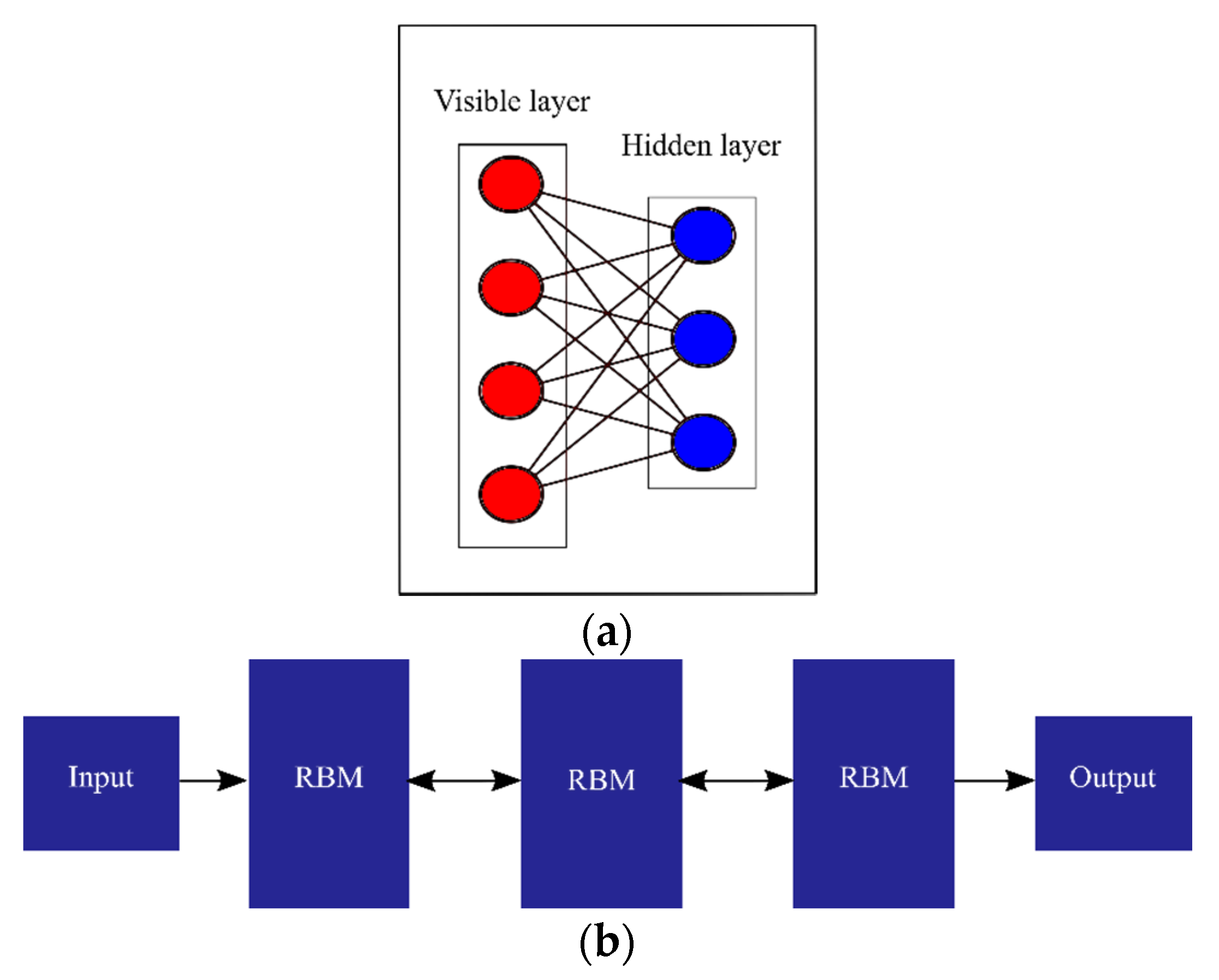
3.1. Deep Belief Network

The deep belief network (DBN) is arguably the first successfully trained DL model. The architecture is constructed of stacked Restricted Boltzmann Machines (RBMs) [46]. A single RBM is an energy-based probabilistic generative model that consists of two connected layers, visible and hidden, with no connections within a layer. The hidden layers are regarded as higher-order features that capture the characteristics of the input data. In multi-layer DBN, the output of the preceding RBM is used as input for the following RBM (Figure 2) allowing for deeper feature extraction and dimension reduction. The training process is done in two steps: firstly, initializing the proper deep network weights by utilizing an efficient unsupervised fast greedy learning strategy; then the final fine-tuning of weights takes place in a supervised manner through Back Propagation, with the addition of a linear classifier on the top layer of the DBN.

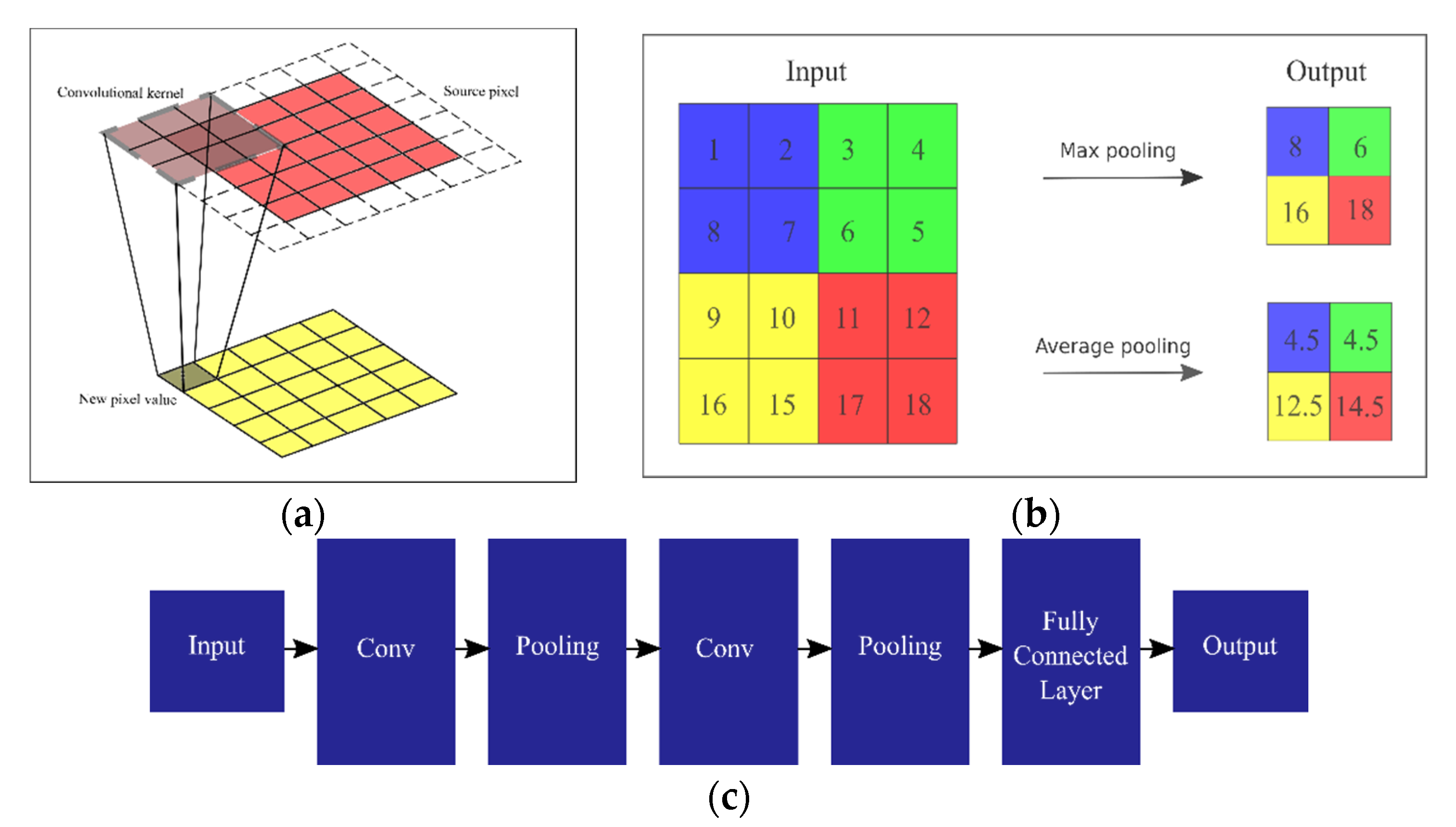
3.2. Convolutional Neural Network

Convolutional Neural Network (CNN) is a type of feedforward deep learning model most commonly used for two-dimensional input data, such as an image. It is the most popular model in computer vision applications, with growing popularity in agriculture [47]. The normal architecture is horizontally hierarchical and constitutes several convolutional, pooling and fully connected layers as presented in Figure 3. Convolutional layers act as feature extractors from the input image, employing kernels or filters. The output dimensionality is then reduced by the pooling layers which extract the most significant features through max pooling or average pooling. The last fully connected layers usually act as classifiers through the softmax function. There have been many other popular architectures such as AlexNet [48] and Visual Geometry Group VGG [49] with different applications and advantages. Recently, 3D CNN has attracted attention in various vision-based applications utilizing image sequences, such as video data [50].

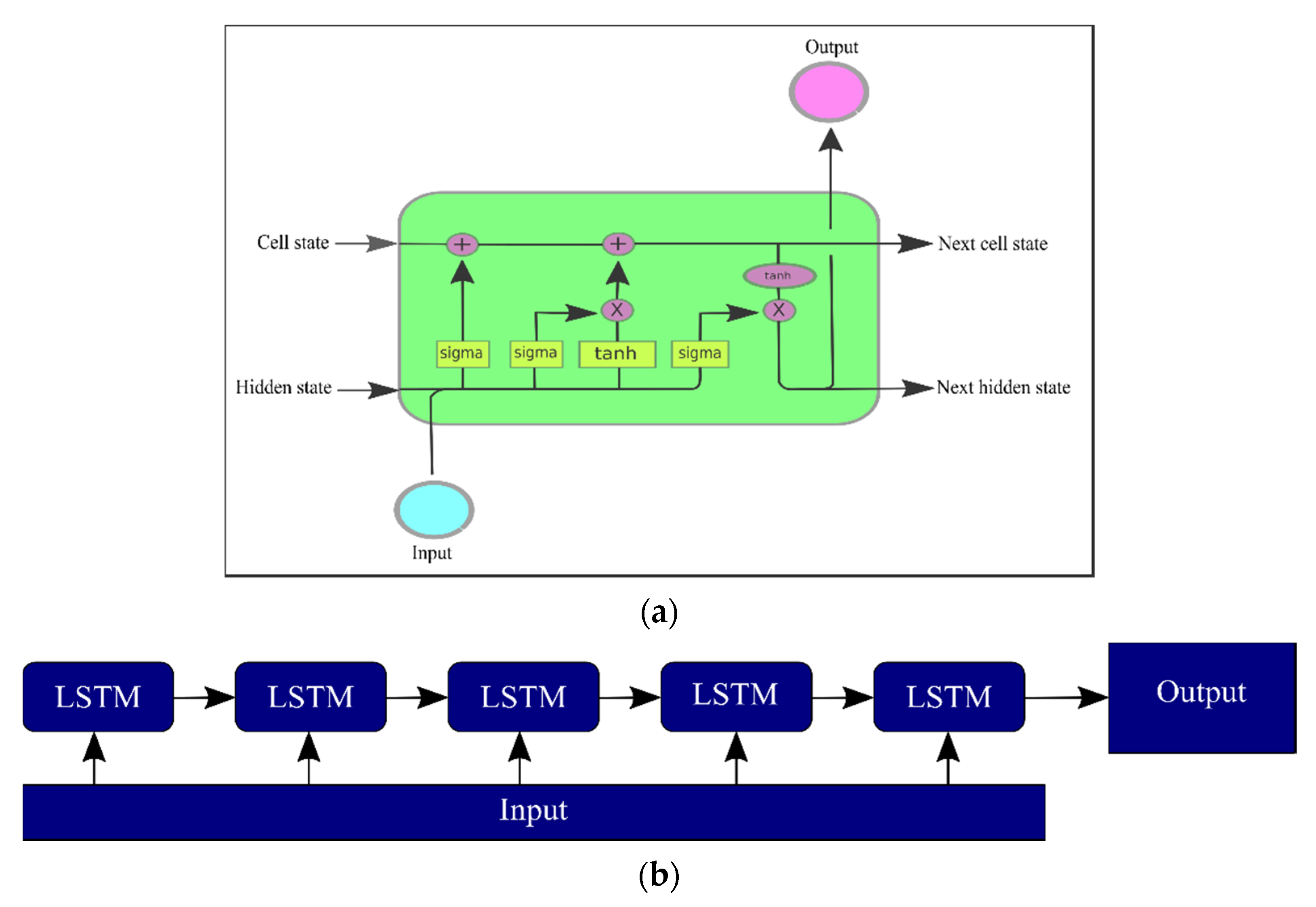
3.3. Long-Short Term Memory Network

Introduced by Hochreiter and Schmidhuber [51], the Long Short-Term Memory (LSTM) network is the augmented version of the Recurrent Neural Network (RNN) used for time series data. RNN was commonly used for discrete sequence analysis through deep feed forward network to learn long-term features; however, it is difficult to store information for very long. LSTM was constructed by adding a memory cell (Figure 4) to overcome the problem of a vanishing gradient in RNN weight training when computed using Backpropagation through time (BPTT) [52]. The cell state allows information to pass through the forget gate layer, input gate layer and output gate layer enabling the recurrent unit to capture long-term information at different time scales. The LSTM model highlights an ability to preserve and learn previous information from long-term time series data through application in natural language processing [53] and speech recognition [54].

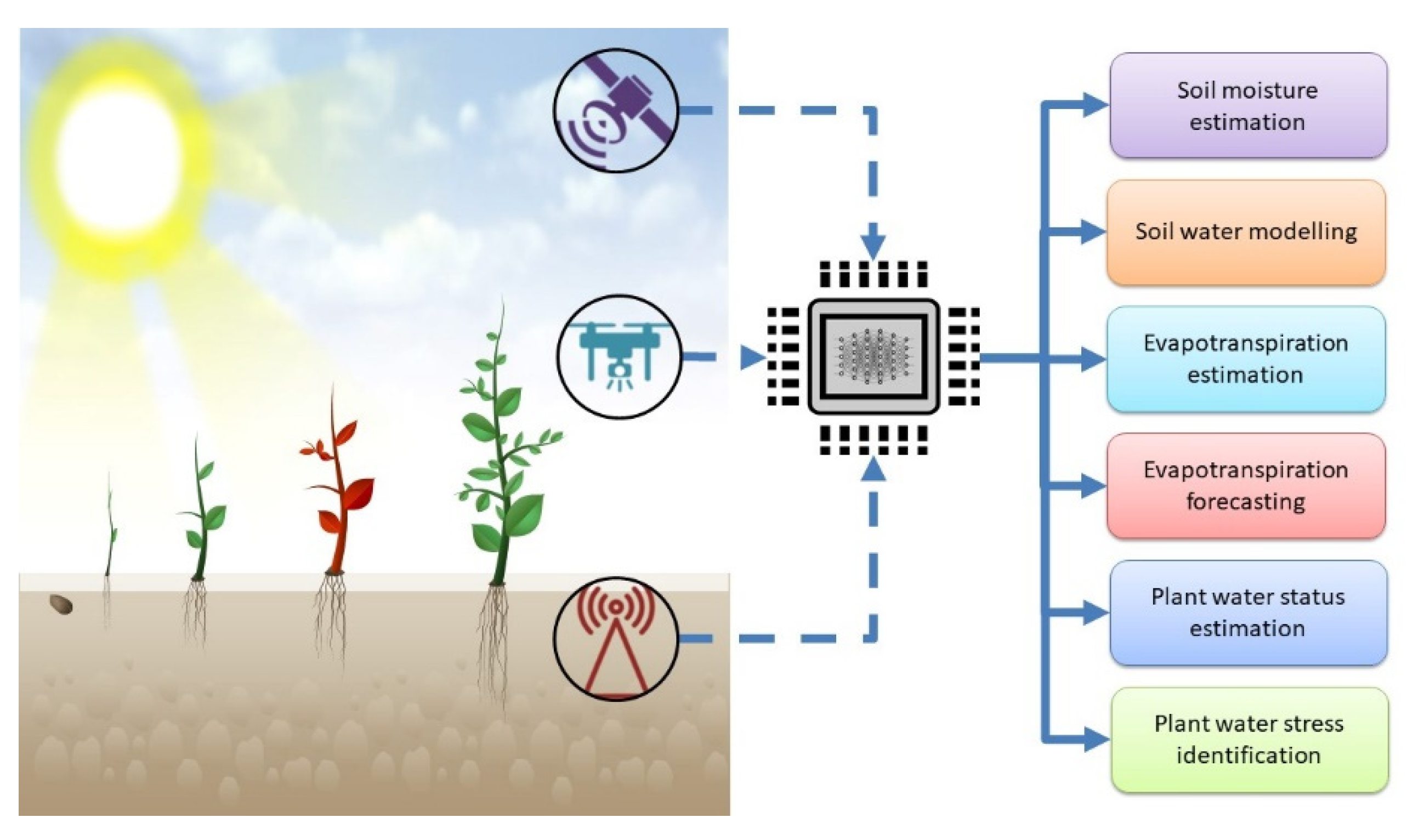
4. Deep Learning in Plant Water Stress Assessment

DL applications were divided into sub-categories via the main methods used in plant water stress assessment including soil moisture estimation, soil water modelling, evapotranspiration estimation, evapotranspiration forecasting, plant water status estimation, and plant water stress identification. The DL techniques used in the reviewed literature are discussed below.

4.1. Soil Moisture Estimation

Soil moisture (SM) is an important parameter for assessing plant water stress as it is directly related to water availability for plant consumption. Over the years, SM measurement has been used for agricultural drought monitoring and irrigation control [55]. It is critical that the percentage of SM does not approach the permanent wilting point, which is the lower limit of plant-available water [56]. The traditional soil sampling few points method for moisture analysis is time-consuming and does not reflect the whole field conditions accurately. In situ measurement, on the other hand, is not feasible for large field application due to the high cost of sensor installation [14]. Advanced remote sensing technique has offered advantages in terms of low-cost and wide scale of monitoring. DL techniques have been used for fast and accurate SM estimation from several remote sensing platforms.
Several studies have used DL for aerial image analysis which could be easily captured using an unmanned aerial vehicle (UAV) or drone for SM estimation. Sobayo et al. [57] proposed a CNN-based regression model to estimate SM content from aerial captured thermal images from three different farm areas. The model was able to predict SM content more accurately than the plain DNN model. The technique shows promising application; however, there is currently a lack of adequate local ground measurement data available at the scale of captured images due to the cost and labour. Tseng et al. [58] tried to overcome the shortcoming by developing an image simulator that can generate pseudo real plant images from the available SM dissipation rate data. The study proposed CNN, which has generated less error in the prediction of soil moisture dissipation rate from the simulated test images in comparison to the traditional ML methods. It also worth noting that the CNN method was robust against the noise introduced into the simulated images.
Large scale SM monitoring has been explored based on satellite observation. DL has been proposed as an alternative to conventional physically-based models developed for SM estimation using satellite data which often perform less well due to limited processing capacity. Zhang et al. [59] used DNN for upscaling in-situ soil moisture estimation using Visible Infrared Imaging Radiometer Suite (VIIRS) raw data records (RDR). The DL model was able to achieve better accuracy than Soil Moisture Active Passive (SMAP) active sensor products and the Global Land Data Assimilation System (GLDAS) model. In another study, Lee et al. [60] also employed DNN to estimate soil moisture over the Korean peninsula using surface and thermal variables from satellite. Compared with Advanced Microwave Scanning Radiometer-2 (AMSR2) and GLDAS SM products, the model showed excellent agreement with the ground measured data.
Wang et al. [61] used DBN to extract features from Fengyun-3D (FY-3D) Medium Resolution Spectral Imager-II (MERSI-II) imagery to estimate soil moisture in the Ningxia Hui Autonomous Region of China. The developed model, called SM-DBN, has outperformed the other conventional models of linear regression (LR) and ANN, based on accuracy performance in correlation with the actual ground measurement data. Ge et al. [62] compared the performance of CNN and conventional ANN for estimating in-situ SM using satellite data of L-band Soil Moisture and Ocean Salinity (SMOS) brightness temperature (TB), C-band Advanced Scatterometer (ASCAT) backscattering coefficients, the Moderate Resolution Imaging Spectroradiometer (MODIS) Normalized Difference Vegetation Index (NDVI), and soil temperature. The results showed that CNN outperformed conventional ANN with better correlation with in-situ soil moisture measurement.

4.2. Soil Water Modelling

Soil water content can be affected by many factors including soil properties, climatic changes, plant growth dynamics, etc., hence it is challenging to determine the soil water content variation accurately and in a timely manner. Modelling the soil water distribution using collected data can be beneficial for predicting in advance the moisture condition in soil by a few days earlier. This will not only support in planning an appropriate irrigation schedule, but can also reduce the impact of drought conditions [63]. However, modelling soil water distribution is not an easy task due to the complex hydrological nature of soil and the correlation with plant and environmental variables. Efficient algorithms are necessary to deal with the nonlinear complex characteristics.
DL has played an important and increasing role in soil water modelling using soil, plant and environmental measurements and has shown better performance than the conventional ML model. Song et al. [64] proposed DBN as feature extraction method combined with the macroscopic cellular automata (MCA) model to simulate spatio-temporal soil hydrological changes in an irrigated corn field using several determining environmental parameters. In comparison to conventional Multilayer Perceptron (MLP), DBN has shown better results for predicting soil water content data, with a reduced error of 18%. Cai et al. [65] used a DNN-based regression model to predict soil moisture at a depth of 20 cm using selected meteorological variables and soil water content data. Comparison with conventional models such as linear regression, support vector machine (SVM), and ANN showed a higher correlation in DNN with the actual data.
Yu et al. [66] proposed a hybrid convolutional neural network-gated recurrent unit (CNN-GRU) for predicting soil moisture in maize root zone using input from soil moisture content and meteorological variables from five different cultivation areas. The validation results showed that CNN-RGU performs better than the CNN and GRU model alone. In an extended forecasting period, the predicted soil moisture from the proposed models were comparable to the sensor-based soil moisture measurements. In another study, Yu et al. [67] investigated further the application of DL models and proposed a combination of a CNN-based Resnet and Bidirectional Long Short-Term Memory (BiLSTM) model for soil water content prediction at four different depths using integrated meteorological, soil water content and growth stage records data for training. The deep learning model had better prediction accuracy than the traditional machine learning models of support vector regression (SVR), MLP and random forest (RF).
DL has also been used for large scale soil moisture prediction based on satellite data such as SMAP. Fang et al. [68] developed LSTM that predicts SMAP level-3 moisture product with atmospheric forcing, model-simulated moisture, and static physiographic attributes as inputs. The results showed that LSTM outperformed conventional methods of multiple linear regression (MLR), autoregressive models (AM) and one-layer ANN. In a more recent study, Fang and Shen [69] further improved the work by introducing a novel data integration (DI) kernel to assimilate the most recent SMAP observations for near-real-time forecast of SM product. The DI-LSTM was compared to the original LSTM model and gave less error in the forecasted values compared to actual measurements.

4.3. Evapotranspiration Estimation

Evapotranspiration (ET) correspond to atmospheric water loss due to plant transpiration and soil evaporation. Crop evapotranspiration (ETc) specifically provides understanding of how fluctuations in climatic parameters can affect plant water consumption under the active phase without restriction from nutritional supply [70]. Measuring field ETc conventionally using a lysimeter is expensive, complex and labour-costly [71]. The FAO-56 [72] model is the well-established method for ETc calculation based on energy and water balance schemes at field scale shown in Equation (1):
ETc = Kc × ETo,
where Kc is the crop coefficient and ETo is the reference evapotranspiration. ETo incorporates the effects of weather into the ETc estimate whilst the properties of the crop which affect ETc are quantified by Kc [73]. ETo is traditionally calculated using the Penman-Montieth (PM) Equation [72] based on measured meteorological sensors. However, the method is limited to the need for large variables.
Deep learning has been used for faster estimation of ETo with limited meteorological variables as inputs. Saggi and Jain [74] used optimized meteorological based processed data as input to DNN for estimation of evapotranspiration values in Punjab, Northern India. Comparison with the standard methods of Generalized Linear Model (GLM), RF, and Gradient-Boosting Machine (GBM) showed DNN’s better performance, providing higher accuracy with the PM-based ETo while avoiding the overfitting issue. In another study, Ferreira and da Cunha [75] proposed that the CNN model showed good performance when used to estimate daily ETo directly from limited hourly meteorological data compared to other models such as RF, extreme gradient boosting (XGBoost), and ANN.
Afzaal et al. [76] used LSTM and BiLSTM for estimating ETo using air temperature and relative humidity as the only variables. Both DL models showed high accuracy compared to the actual ETo, with less difference in performance between the two models. Chen et al. [77] evaluate the performance of three DL methods of deep DNN, temporal convolution network (TCN) [78], and long short-term memory neural network (LSTM) for reference evapotranspiration estimation. The results showed that DL model outperformed other conventional models, and TCN and LSTM showed outstanding performance when temperature features were used.
Recently, remote sensing has been used for large scale ET estimation providing high spatial and temporal resolution. Several models and algorithms, such as Mapping evapotranspiration at high resolution with internalized calibration (METRIC), the Two-source energy balance (TSEB) model, and machine learning have been used and discussed [79]. Recently, DL learning has been introduced to improve the ET estimation based on remotely sensed data. Cui et al. [80] developed a gap-filling algorithm based on the temperature surface-vegetation index (TSVI) model to provide continuous daily actual ET estimation at regional scale. Results showed good correlation between the estimated ET from TSVI-DNN model with ground observation. García-Pedrero, et al. [81], for the first time, introduced CNN for estimating spatially distributed ET using remote sensing data without the need of a surface energy model. Comparison with data from METRIC showed satisfactory ET maps were produced by the CNN.
At individual plant scale, stress variation is expressed directly in plant transpiration (T). Measuring plant transpiration can give better understanding of the relation between plant stress and the environment. However, direct measurement of T by sap flow is expensive, difficult and time-consuming. Several studies have used DL for plant transpiration estimation using a sensory measured environmental variable. Shuaishuai et al. [82] have utilized DBN and least square support vector machine (LSSVM) to directly predict the leaf transpiration rate of strawberry in a greenhouse environment. DBN-LSSVM model outperformed two conventional models with higher prediction accuracy suggesting DBN as an efficient feature extractor. Fan et al. [83] compares several ML algorithms of SVM, XGBoost, and ANN, including DNN, for estimating maize transpiration using meteorological variables, soil water and leaf area index as inputs. The result showed DNN outperformed other techniques by a slight margin.

4.4. Evapotranspiration Forecasting

ET forecasting can bring important insights into future climate conditions which can be beneficial in assessing plant water stress and irrigation planning. It can also compensate for the lack of data generated, due to less sensors being installed as a result of high cost and limited manpower. Recently, DL ability to consider temporal features in the data has been utilized for accurate ET forecasting. Ferreira and da Cunha [84] proposed a CNN-LSTM combination for multi-step ahead prediction of daily ETo with relatively good performance achieved in comparison with traditional ML models and CNN and LSTM alone. Lucas et al. [85] also explored the use of three different architectures of CNN in the prediction of ETo time series. Using real climatic data, the models were able to predict daily ETo with lower uncertainty. Yin et al. [86], on the other hand, considered a hybrid BiLSTM to forecast short-term daily ETo from meteorological data collected in the semi-arid region of central Ningxia, China. The results showed that the model was able to improve the forecast performance constantly compared to the general model.
DL has also been investigated as a highly capable techniques for ETc forecasting based on historical field measurement data. Chen et al. [87] conducted an attempt to estimate ETc for maize using two-years field measurements of ETc data using a lysimeter and TCN. The new form of DL, comprised of LSTM and DNN, was able to estimate maize ETc based on plant height, air temperature, relative humidity, solar radiation, leaf-area index and soil temperature better than the DNN and LSTM method alone. Elbeltagi, et al. [88] used the DNN model to estimate and predict ETc for several locations of wheat cultivation in Egypt based on recorded historical and future meteorological data. The results showed high correlation between ETc values from the standard FAO-56 method and the values predicted from the DL model.

4.5. Plant Water Status Estimation

Many techniques have been developed over the years to describe plant water status (PWS) such as relative water content (RWC) [89], equivalent water thickness (EWT) and fuel moisture content (FWC) [90]. Other techniques are based on the changes in the plant physical system as a response to water content, such as stem diameter variations (SD) [91,92]. These parameters have been used as indicators for assessing plant conditions related to drought (as water stress index) and irrigation management [93]. Recent progress has seen remote sensing measurement estimate plant water status non-destructively with various modelling methods have used to correlate the measurement and ground measured plant water status, ranging from simple linear regression to machine learning technique [94,95,96].
The DL model is currently being investigated as a fast and robust method for PWS estimation using aggregated data collected from various sensory measurements. Fariñas et al. [97] evaluated CNN and the Random forest (RF) technique as regression model to estimate RWC in plant leaf from the transmission coefficient of frequency data collected using Non-contact resonant ultrasound spectroscopy (NC-RUS). The CNN technique utilizes the entire ultrasonic spectra collected non-invasively from the leaf while RF takes only four relevant input spectra resulting in better performance of the CNN model as shown by the higher correlation and lower median prediction error.
DL has also been used to extract features from multi-modal data to increase inversion performance. Kaneda et al. [98] combined environmental measurements with leaf wilting features extracted from plant images using a CNN-based model as multi-modal feature extractor to predict changes in stem diameter to assess water status in the tomato plant. Comparison of several conventional regression algorithms showed the superiority of the proposed model due to its low prediction error. The method proposed, however, has not considered the temporal aspect of the data which could further increase the prediction accuracy. In more recent years, Wakamori et al. [99] improved the existing work by proposing an LSTM network with clustering-based drop (C-Drop). The C-Drop neural network supports the regression analysis by giving the environmental feature an equal consideration. Based on the results, the new proposed model improved the prediction accuracy by 21% compared to the previous method.
Plant spectral information has been used to estimate PWS based on the developed vegetation indices techniques, such as WI and NDWI [100]. Moreover, ML has been widely investigated as the method used in the process of finding the relevant spectral bands that give high correlation with the PWS parameters [90,101,102,103,104]. DL, however, has been hardly applied to this problem. Rehman et al. [105] were possibly the first to have used a 1D-convolutional neural network to extract the mean spectral reflectance from the hyperspectral image to predict RWC in maize. The model based on the updated Inception module called DeepRWC was able to learn the features from hyperspectral data without the need for spectral selection or dimensionality reduction. DeepRWC achieved better accuracy in comparison with the two standard approaches of partial least square regression (PLSR) and SVM.
In another study, Rao et al. [106] have integrated a physical model with RNN to accurately predict live moisture fuel content (LMFC), defined as the mass of canopy leaf water per unit of dry biomass, which is a key parameter for assessing wildfire risk. The model takes input variables from microwave remote sensing of Sentinel-1 backscatter and Landsat-8 optical reflectance, with additional soil properties, for training on LFMC field samples. They found that the DL model performance exceeds the conventional process-based methods and that precision can be improved with the addition of the microwave RS data.

4.6. Plant Water Stress Identification

Plant water stress identification refers to water stress detection in plants by distinguishing water stress and non-water stress in the labelled plant. A computer vision system for plant water stress identification has been developed over the years using conventional ML algorithms such as ANN [107], Adaptive neuro-fuzzy classifier [108], and Gradient boosting decision tree (GBDT) [109]. However, the need for feature extraction from the images and for selection of conventional ML has limited the performance of the analysis.
DL superiority in image recognition by automatically learning from patterns has been leveraged in plant water stress identification, with CNN becoming the standard model for automated feature extraction and transformation. An et al. [110] were possibly the first who attempted to identify plant water stress in maize using pre-trained CNN: Resnet50 and Resnet120 based on three treatments of stress: optimum moisture, light drought, and moderate drought stress. The performances of the models showed between 91–98% accuracy with the fastest training time close to 8 min. Compared to manually extracted features and classification using the conventional GBDT model, CNN performs better with Resnet50 showing the highest accuracy.
Jiang et al. [111] attempted to improve the performance of the identification by introducing a Gabor filter to extract texture features from the same dataset used in [110] for the Zhengdan maize variety and reduced the dimension before feeding to the pre-trained CNN model of Alexnet. The results showed slight improvement in the model accuracy but with good adaptation to illumination changes and angle transformation. Zhuang et al. [112] further investigated the Zhengdan maize dataset by designing their own CNN architecture, that was relatively simple but efficient in feature extraction, by selecting the most relevant feature maps. The proposed method used SVM as final classifier and the results showed better accuracy achieved in comparison with the other well-known CNN models of VGG16, ResNet50, Xception and xPLNet.
Chandel et al. [113] evaluated instead the three different popular CNN models of AlexNet, GoogLeNet and Inception V3 for plant water stress classification of maize, okra and soybean images collected from different growth stages. The performance of GoogLeNet was found to be superior compared to others with an accuracy of 98.3%, 97.5% and 94.1% for maize, okra and soybean, respectively.
Realizing the potential of CNN as an image classifier for plant water stress identification, recent studies have been assessing the applicability of such techniques to be used in field conditions. Plant images were collected at certain heights providing wide monitoring of multiple plants under the same cultivation area. Soffer et al. [114] used the pre-trained CNN of VGG16 for real time classification of water stress treatment of five different groups of corn. The proposed method used the image data concatenated with the plant images as an input to the DL model. The results showed excellent accuracy for five treatment classifications, although most studies showed less performance when dealing with a higher number of classes. Freeman, et al. [115] assessed the use of cloud-based CNN training to identify plant water stress across six container-grown ornamental shrub species. Using near infrared images captured in the field from small, unmanned aircraft system (sUAS), the framework was able to achieve high accuracy performance despite constraints of small sample size, low image resolution, and lack of clear visual differences.
Although CNN is the most commonly used model in image processing, the sequential characteristic of the time-series image is not considered in the previous classification tasks. The temporal dependence relationship of a specific plant growth period may hold information that can be used for water stress identification. In consideration of the temporal feature, Li et al. [116] applied for the first time BiLSTM networks to extract features from sequential digital images of maize and sorghum. BiLSTM has shown good performance for plant water stress identification compared to the vanilla CNN, LSTM and RNN model. They also found that BiLSTM can identify plant water stress at an early stage and with mild stress, where less variations can be noted in the plant. Table 1 is the compilation of the highlighted methods, input data, models with remarks based on DL applications.

5. Discussion and Future Perspectives

Deep learning is a powerful and versatile tool that can be applied to solve a wide range of problems either through regression or classification analysis. The superior performance compared to conventional ML makes it a suitable method for modelling highly complex plant water stress conditions. Remote sensing is another advanced method with much potential in plant water stress assessment, providing high spatial, temporal and spectral resolution. However, it has been noted that DL application in remote sensing plant water stress assessment is still at the initial stage of development. This is especially true in the case of ETc estimation. Many strategies can still be explored and a few studies have started to pave the way in utilizing DL for solving problems in the remote sensing application in reference to ET estimation [80,81,117].
Remote sensing thermal and hyperspectral images have been extensively investigated for plant water stress assessment based on vegetation indices and the crop water stress index technique. However, challenges remain regarding the effect of plant geometric structure and image background which could influence the analysis. RGB image has been proposed for remote sensing estimation of plant water content estimation utilizing morphological features (Leaf Area) [118,119] and colour [120] to estimate plant physiological response to water stress. It is preferable due to the low-cost and easy to use sensor [120]. DL has been successfully used for segmenting plant and background in RGB images for plant water stress detection with good results [121]. However, lack of spectral bands, with only three basic colours in the image, limits detailed information about the status of the plant [122]. Khan et al. [123] proposed an innovative approach to using DL for predicting vegetation index from an RGB aerial image. The development shows that it is possible to have a low-cost and efficient method for plant water stress assessment while improving agricultural production with the help of an advanced algorithm such as DL.
The inherent bottleneck of the DL technique has always been the size and quality of the datasets available for training and validating the model. Data collected through remote sensing mostly involves images, and although satellite-based images are commercially available, data on aerial plant images under water stress is limited leading most of the studies to use self-collected images while adopting transfer learning in their application. Transfer learning is a method of using a pre-trained model for other applications which can be used to train a new model from scratch using available models. It has already been successfully used for solving the problem of small sample size with improved accuracy. For a robust model to be developed, large varieties of datasets are required including data collected from different sensors and plant species.
Despite successful applications and superior performance achieved relative to conventional ML methods, DL utilization in water stress assessment is still at the beginning phase and there is still a lot to explore. Some of the future prospects are discussed together with the possible key issues.

5.1. Deep Learning for 3-Dimensional Data

The combination of deep learning and 3D data thus far has been infrequently explored despite the possibilities of improving assessment. Most studies have only used either one or two-dimensional data with the DL processing algorithm. Integration of data from soil, atmospheric and plant-based measurements would create a three-dimensional input that can improve the accuracy of assessment [14].
Furthermore, there are sensors that can collect three-dimensional data that can generate more information for plant water stress assessment. For example, a hyperspectral image which contains spatial and spectral information can simultaneously be utilized for accurately assessing plant water status. Joint spectral and spatial information from remote sensing data has been utilized for improved the prediction task using a deep learning approach [124,125]. The application of 3D digital RGB image data to DL is also foreseeable in the future as a 3D image can be used to extract features like the bending angle of a leaf that can be related to water stress [99].
Using advanced data can come with challenges. Firstly, the inaccuracies in 3D image reconstruction can affect the features extracted by the DL model resulting in subpar performance. Secondly, the high cost of the advanced sensors might limit the adoptability of such a method. This in turn will reduce the data production which then might further limit the much-needed data varieties pertinent to the successful learning of the DL model.

5.2. Plant Varieties Challenge

Varieties of plant species have always been a challenge when using ML for plant water stress detection. A specific model developed for a particular plant species usually does not hold the same accuracy when trained with other varieties, as the physiological responses of plants to water stress and their relative importance for crop productivity vary with species, soil type, nutrients and climate [115].
There is also the need to study the effect of variations that occur within the same species but cultivated in different locations. Although plants may look similar, they vary widely in both shape, chemical composition and the concentration of water in the leaf intercellular spaces due to environmental influences. Thus far no study has been found to have investigated this case, although the result can be significant for improving the scalability of the technique. Theoretically, DL’s huge learning capabilities can be used to cater for plant varieties provided sufficient data is available. Khaki et al. [126] have used CNN to identify corn hybrids based on tolerance to environmental stress from the inputs of yield, soil and weather data.
Unfortunately, unbalanced data can occur due to the fact that isohydric plants have better control mechanisms for lack of water and can last longer, while anisohydric plants which have a less effective control mechanism will die within days without water [127], although the use of a deep learning model of Generative Adversary Network (GAN) may provide the required dataset through synthetically generated data [128].

6. Conclusions

This paper presents a comprehensive review of plant water stress assessment in which cutting-edge sensor fusion technologies have been applied at a rapid pace contributing significantly towards improving agricultural production, plant breeding, efficient agricultural water consumption and a fast method for monitoring forest wildfires. Huge and complex data generated from the sensors require advanced analytical algorithms for processing data representation. Deep learning sensor fusion as a state-of-the-art technique has been implemented as model inversion for the estimation of plant water stress parameters and identification. As seen from the literature, DL’s high learning capability is definitely useful for fast processing of field data from multisource sensors. DL was also successfully applied as an advanced tool for image processing with huge potential for fast detection of plant water stress in the field. However, sufficient datasets and variations of sample are required for creating a robust method. Combining DL with an advanced data type such as 3D image can be considered for increasing this accuracy.

Author Contributions

Conceptualization, M.H.K. and Z.H.I.; writing—original draft preparation, M.H.K.; writing—review and editing, Z.H.I. and N.B.S.; visualization, M.H.K.; supervision, Z.H.I. All authors have read and agreed to the published version of the manuscript.

Funding

This work was supported by Ministry of Higher Education and Universiti Teknologi Malaysia under Grant no. R.K130000.7843.5F348 and Q.K130000.2543.19H97.

Informed Consent Statement

Not applicable.

Acknowledgments

The authors gratefully thank Raudah Yunus for her assistance with the preparation of the manuscript.

Conflicts of Interest

The authors declare no conflict of interest.

References

  1. Osakabe, Y.; Osakabe, K.; Shinozaki, K.; Tran, L.-S. Response of plants to water stress. Front. Plant Sci. 2014, 5. [Google Scholar] [CrossRef] [PubMed] [Green Version]
  2. Kashyap, P.; Panda, R. Effect of irrigation scheduling on potato crop parameters under water stressed conditions. Agric. Water Manag. 2003, 59, 49–66. [Google Scholar] [CrossRef]
  3. Lisar, S.Y.; Motafakkerazad, R.; Hossain, M.M.; Rahman, I.M. Water stress in plants: Causes, effects and responses. In Water Stress; InTech: London, UK, 2012. [Google Scholar]
  4. Byrareddy, V.; Kouadio, L.; Kath, J.; Mushtaq, S.; Rafiei, V.; Scobie, M.; Stone, R. Win-win: Improved irrigation management saves water and increases yield for robusta coffee farms in Vietnam. Agric. Water Manag. 2020, 241, 106350. [Google Scholar] [CrossRef]
  5. Kriston-Vizi, J.; Umeda, M.; Miyamoto, K. Assessment of the water status of mandarin and peach canopies using visible multispectral imagery. Biosyst. Eng. 2008, 100, 338–345. [Google Scholar] [CrossRef] [Green Version]
  6. Chai, Q.; Gan, Y.; Zhao, C.; Xu, H.-L.; Waskom, R.M.; Niu, Y.; Siddique, K.H. Regulated deficit irrigation for crop production under drought stress. A review. Agron. Sustain. Dev. 2016, 36, 3. [Google Scholar] [CrossRef] [Green Version]
  7. Stagakis, S.; González-Dugo, V.; Cid, P.; Guillén-Climent, M.L.; Zarco-Tejada, P.J. Monitoring water stress and fruit quality in an orange orchard under regulated deficit irrigation using narrow-band structural and physiological remote sensing indices. ISPRS J. Photogramm. Remote Sens. 2012, 71, 47–61. [Google Scholar] [CrossRef] [Green Version]
  8. Chuvieco, E.; Cocero, D.; Riano, D.; Martin, P.; Martınez-Vega, J.; de la Riva, J.; Perez, F. Combining NDVI and surface temperature for the estimation of live fuel moisture content in forest fire danger rating. Remote Sens. Environ. 2004, 92, 322–331. [Google Scholar] [CrossRef]
  9. Oumar, Z.; Mutanga, O. Predicting water stress induced by Thaumastocoris peregrinus infestations in plantation forests using field spectroscopy and neural networks. J. Spat. Sci. 2014, 59, 79–90. [Google Scholar] [CrossRef]
  10. Munns, R.; James, R.A.; Sirault, X.R.; Furbank, R.T.; Jones, H.G. New phenotyping methods for screening wheat and barley for beneficial responses to water deficit. J. Exp. Bot. 2010, 61, 3499–3507. [Google Scholar] [CrossRef] [Green Version]
  11. Bolten, J.D.; Crow, W.T.; Zhan, X.; Jackson, T.J.; Reynolds, C.A. Evaluating the utility of remotely sensed soil moisture retrievals for operational agricultural drought monitoring. IEEE J. Sel. Top. Appl. Earth Obs. Remote Sens. 2009, 3, 57–66. [Google Scholar] [CrossRef] [Green Version]
  12. Padhee, S.K.; Nikam, B.R.; Dutta, S.; Aggarwal, S.P. Using satellite-based soil moisture to detect and monitor spatiotemporal traces of agricultural drought over Bundelkhand region of India. Giscience Remote Sens. 2017, 54, 144–166. [Google Scholar] [CrossRef]
  13. Brillante, L.; Mathieu, O.; Lévêque, J.; Bois, B. Ecophysiological modeling of grapevine water stress in burgundy terroirs by a machine-learning approach. Front. Plant Sci. 2016, 7, 796. [Google Scholar] [CrossRef]
  14. Ihuoma, S.O.; Madramootoo, C.A. Recent advances in crop water stress detection. Comput. Electron. Agric. 2017, 141, 267–275. [Google Scholar] [CrossRef]
  15. Kramer, P.J. Water Stress and Plant Growth 1. Agron. J. 1963, 55, 31–35. [Google Scholar] [CrossRef]
  16. Lee, W.; Alchanatis, V.; Yang, C.; Hirafuji, M.; Moshou, D.; Li, C. Sensing technologies for precision specialty crop production. Comput. Electron. Agric. 2010, 74, 2–33. [Google Scholar] [CrossRef]
  17. Gerhards, M.; Schlerf, M.; Mallick, K.; Udelhoven, T. Challenges and Future Perspectives of Multi-/Hyperspectral Thermal Infrared Remote Sensing for Crop Water-Stress Detection: A Review. Remote Sens. 2019, 11, 1240. [Google Scholar] [CrossRef] [Green Version]
  18. Alvino, A.; Marino, S. Remote sensing for irrigation of horticultural crops. Horticulturae 2017, 3, 40. [Google Scholar] [CrossRef] [Green Version]
  19. Virnodkar, S.S.; Pachghare, V.K.; Patil, V.; Jha, S.K. Remote sensing and machine learning for crop water stress determination in various crops: A critical review. Precis. Agric. 2020, 21, 1121–1155. [Google Scholar] [CrossRef]
  20. Liakos, K.G.; Busato, P.; Moshou, D.; Pearson, S.; Bochtis, D. Machine Learning in Agriculture: A Review. Sensors 2018, 18, 2674. [Google Scholar] [CrossRef] [Green Version]
  21. Chlingaryan, A.; Sukkarieh, S.; Whelan, B. Machine learning approaches for crop yield prediction and nitrogen status estimation in precision agriculture: A review. Comput. Electron. Agric. 2018, 151, 61–69. [Google Scholar] [CrossRef]
  22. Ma, L.; Liu, Y.; Zhang, X.; Ye, Y.; Yin, G.; Johnson, B.A. Deep learning in remote sensing applications: A meta-analysis and review. ISPRS J. Photogramm. Remote Sens. 2019, 152, 166–177. [Google Scholar] [CrossRef]
  23. Kussul, N.; Lavreniuk, M.; Skakun, S.; Shelestov, A. Deep Learning Classification of Land Cover and Crop Types Using Remote Sensing Data. IEEE Geosci. Remote Sens. Lett. 2017, 14, 778–782. [Google Scholar] [CrossRef]
  24. Yuan, Q.; Shen, H.; Li, T.; Li, Z.; Li, S.; Jiang, Y.; Xu, H.; Tan, W.; Yang, Q.; Wang, J. Deep learning in environmental remote sensing: Achievements and challenges. Remote Sens. Environ. 2020, 241, 111716. [Google Scholar] [CrossRef]
  25. Mochida, K.; Koda, S.; Inoue, K.; Hirayama, T.; Tanaka, S.; Nishii, R.; Melgani, F. Computer vision-based phenotyping for improvement of plant productivity: A machine learning perspective. GigaScience 2018, 8, giy153. [Google Scholar] [CrossRef] [Green Version]
  26. Kamilaris, A.; Prenafeta-Boldú, F.X. Deep learning in agriculture: A survey. Comput. Electron. Agric. 2018, 147, 70–90. [Google Scholar] [CrossRef] [Green Version]
  27. Gao, Z.; Luo, Z.; Zhang, W.; Lv, Z.; Xu, Y. Deep Learning Application in Plant Stress Imaging: A Review. AgriEngineering 2020, 2, 29. [Google Scholar] [CrossRef]
  28. Singh, A.K.; Ganapathysubramanian, B.; Sarkar, S.; Singh, A. Deep learning for plant stress phenotyping: Trends and future perspectives. Trends Plant Sci. 2018, 23, 883–898. [Google Scholar] [CrossRef] [PubMed] [Green Version]
  29. Noon, S.K.; Amjad, M.; Qureshi, M.A.; Mannan, A. Use of Deep Learning Techniques for Identification of Plant Leaf Stresses: A Review. Sustain. Comput. Inform. Syst. 2020, 28, 100443. [Google Scholar]
  30. Hinton, G.E.; Salakhutdinov, R.R. Reducing the dimensionality of data with neural networks. Science 2006, 313, 504–507. [Google Scholar] [CrossRef] [Green Version]
  31. Deng, L.; Yu, D. Deep learning: Methods and applications. Found. Trends Signal Process. 2014, 7, 197–387. [Google Scholar] [CrossRef] [Green Version]
  32. Schmidhuber, J. Deep learning in neural networks: An overview. Neural Netw. 2015, 61, 85–117. [Google Scholar] [CrossRef] [Green Version]
  33. Geng, L.; Dong, T. An agricultural monitoring system based on wireless sensor and depth learning algorithm. Int. J. Online Eng. 2017, 13, 127–137. [Google Scholar] [CrossRef] [Green Version]
  34. García-Mateos, G.; Hernández-Hernández, J.L.; Escarabajal-Henarejos, D.; Jaén-Terrones, S.; Molina-Martínez, J.M. Study and comparison of color models for automatic image analysis in irrigation management applications. Agric. Water Manag. 2015, 151, 158–166. [Google Scholar] [CrossRef]
  35. Hendrawan, Y.; Murase, H. Neural-intelligent water drops algorithm to select relevant textural features for developing precision irrigation system using machine vision. Comput. Electron. Agric. 2011, 77, 214–228. [Google Scholar] [CrossRef]
  36. Kim, Y.; Glenn, D.M.; Park, J.; Ngugi, H.K.; Lehman, B.L. Hyperspectral image analysis for water stress detection of apple trees. Comput. Electron. Agric. 2011, 77, 155–160. [Google Scholar] [CrossRef]
  37. Gutiérrez, S.; Diago, M.P.; Fernández-Novales, J.; Tardaguila, J. Vineyard water status assessment using on-the-go thermal imaging and machine learning. PLoS ONE 2018, 13, e0192037. [Google Scholar] [CrossRef] [PubMed]
  38. Boxel, D.V. Hands-On Deep Learning with TensorFlow; Packt Publishing: Birmingham, UK, 2017. [Google Scholar]
  39. Ketkar, N.; Santana, E. Deep Learning with Python; Springer: Berlin/Heidelberg, Germany, 2017; Volume 1. [Google Scholar]
  40. Bisong, E. Google Colaboratory. In Building Machine Learning and Deep Learning Models on Google Cloud Platform: A Comprehensive Guide for Beginners; Apress: Berkeley, CA, USA, 2019; pp. 59–64. [Google Scholar] [CrossRef]
  41. Carneiro, T.; Da Nóbrega, R.V.M.; Nepomuceno, T.; Bian, G.-B.; De Albuquerque, V.H.C.; Reboucas Filho, P.P. Performance analysis of google colaboratory as a tool for accelerating deep learning applications. IEEE Access 2018, 6, 61677–61685. [Google Scholar] [CrossRef]
  42. Ubbens, J.R.; Stavness, I. Deep plant phenomics: A deep learning platform for complex plant phenotyping tasks. Front. Plant Sci. 2017, 8, 1190. [Google Scholar] [CrossRef] [PubMed] [Green Version]
  43. Ghosal, S.; Blystone, D.; Singh, A.K.; Ganapathysubramanian, B.; Singh, A.; Sarkar, S. An explainable deep machine vision framework for plant stress phenotyping. Proc. Natl. Acad. Sci. USA 2018, 115, 4613–4618. [Google Scholar] [CrossRef] [Green Version]
  44. Fahlgren, N.; Feldman, M.; Gehan, M.A.; Wilson, M.S.; Shyu, C.; Bryant, D.W.; Hill, S.T.; McEntee, C.J.; Warnasooriya, S.N.; Kumar, I. A versatile phenotyping system and analytics platform reveals diverse temporal responses to water availability in Setaria. Mol. Plant 2015, 8, 1520–1535. [Google Scholar] [CrossRef] [Green Version]
  45. Feldman, M.J.; Paul, R.E.; Banan, D.; Barrett, J.F.; Sebastian, J.; Yee, M.-C.; Jiang, H.; Lipka, A.E.; Brutnell, T.P.; Dinneny, J.R. Time dependent genetic analysis links field and controlled environment phenotypes in the model C4 grass Setaria. PLoS Genet. 2017, 13, e1006841. [Google Scholar] [CrossRef] [Green Version]
  46. Hinton, G.E.; Osindero, S.; Teh, Y.-W. A fast learning algorithm for deep belief nets. Neural Comput. 2006, 18, 1527–1554. [Google Scholar] [CrossRef]
  47. Kamilaris, A.; Prenafeta-Boldú, F. A review of the use of convolutional neural networks in agriculture. J. Agric. Sci. 2018, 156, 312–322. [Google Scholar] [CrossRef] [Green Version]
  48. Krizhevsky, A.; Sutskever, I.; Hinton, G.E. Imagenet classification with deep convolutional neural networks. Adv. Neural Inf. Process. Syst. 2012, 25, 1097–1105. [Google Scholar] [CrossRef]
  49. Simonyan, K.; Zisserman, A. Very deep convolutional networks for large-scale image recognition. arXiv 2014, arXiv:1409.1556. [Google Scholar]
  50. Tran, D.; Bourdev, L.; Fergus, R.; Torresani, L.; Paluri, M. Learning spatiotemporal features with 3d convolutional networks. In Proceedings of the IEEE International Conference on Computer Vision, Santiago, Chile, 7–13 December 2015; pp. 4489–4497. [Google Scholar]
  51. Hochreiter, S.; Schmidhuber, J. Long short-term memory. Neural Comput. 1997, 9, 1735–1780. [Google Scholar] [CrossRef] [PubMed]
  52. Werbos, P.J. Backpropagation through time: What it does and how to do it. Proc. IEEE 1990, 78, 1550–1560. [Google Scholar] [CrossRef] [Green Version]
  53. Mikolov, T.; Kombrink, S.; Burget, L.; Černocký, J.; Khudanpur, S. Extensions of recurrent neural network language model. In Proceedings of the 2011 IEEE International Conference on Acoustics, Speech and Signal Processing (ICASSP), Prague, Czech Republic, 22–27 May 2011; pp. 5528–5531. [Google Scholar]
  54. Graves, A.; Mohamed, A.-R.; Hinton, G. Speech recognition with deep recurrent neural networks. In Proceedings of the 2013 IEEE International Conference on Acoustics, Speech and Signal Processing, Vancouver, BC, Canada, 26–31 May 2013; pp. 6645–6649. [Google Scholar]
  55. Steppe, K.; De Pauw, D.J.W.; Lemeur, R. A step towards new irrigation scheduling strategies using plant-based measurements and mathematical modelling. Irrig. Sci. 2008, 26, 505. [Google Scholar] [CrossRef]
  56. Yamaç, S.S.; Şeker, C.; Negiş, H. Evaluation of machine learning methods to predict soil moisture constants with different combinations of soil input data for calcareous soils in a semi arid area. Agric. Water Manag. 2020, 234, 106121. [Google Scholar] [CrossRef]
  57. Sobayo, R.; Wu, H.; Ray, R.; Qian, L. Integration of Convolutional Neural Network and Thermal Images into Soil Moisture Estimation. In Proceedings of the 2018 1st International Conference on Data Intelligence and Security (ICDIS), South Padre Island, TX, USA, 8–10 April 2018; pp. 207–210. [Google Scholar]
  58. Tseng, D.; Wang, D.; Chen, C.; Miller, L.; Song, W.; Viers, J.; Vougioukas, S.; Carpin, S.; Ojea, J.A.; Goldberg, K. Towards Automating Precision Irrigation: Deep Learning to Infer Local Soil Moisture Conditions from Synthetic Aerial Agricultural Images. In Proceedings of the 2018 IEEE 14th International Conference on Automation Science and Engineering (CASE), Munich, Germany, 20–24 August 2018; pp. 284–291. [Google Scholar]
  59. Zhang, D.; Zhang, W.; Huang, W.; Hong, Z.; Meng, L. Upscaling of surface soil moisture using a deep learning model with VIIRS RDR. ISPRS Int. J. Geo-Inf. 2017, 6, 130. [Google Scholar] [CrossRef]
  60. Lee, C.S.; Sohn, E.; Park, J.D.; Jang, J.-D. Estimation of soil moisture using deep learning based on satellite data: A case study of South Korea. Giscience Remote Sens. 2019, 56, 43–67. [Google Scholar] [CrossRef]
  61. Wang, W.; Zhang, C.; Li, F.; Song, J.; Li, P.; Zhang, Y. Extracting Soil Moisture from Fengyun-3D Medium Resolution Spectral Imager-II Imagery by Using a Deep Belief Network. J. Meteorol. Res. 2020, 34, 748–759. [Google Scholar] [CrossRef]
  62. Ge, L.; Hang, R.; Liu, Y.; Liu, Q. Comparing the performance of neural network and deep convolutional neural network in estimating soil moisture from satellite observations. Remote Sens. 2018, 10, 1327. [Google Scholar] [CrossRef] [Green Version]
  63. Adeyemi, T.; Grove, I.; Peets, S.; Domun, Y.; Norton, T. Dynamic Neural Network Modelling of Soil Moisture Content for Predictive Irrigation Scheduling. Sensors 2018, 18, 3408. [Google Scholar] [CrossRef] [PubMed] [Green Version]
  64. Song, X.; Zhang, G.; Liu, F.; Li, D.; Zhao, Y.; Yang, J. Modeling spatio-temporal distribution of soil moisture by deep learning-based cellular automata model. J. Arid Land 2016, 8, 734–748. [Google Scholar] [CrossRef] [Green Version]
  65. Cai, Y.; Zheng, W.; Zhang, X.; Zhangzhong, L.; Xue, X. Research on soil moisture prediction model based on deep learning. PLoS ONE 2019, 14, e0214508. [Google Scholar] [CrossRef] [PubMed]
  66. Yu, J.; Zhang, X.; Xu, L.; Dong, J.; Zhangzhong, L. A hybrid CNN-GRU model for predicting soil moisture in maize root zone. Agric. Water Manag. 2020, 245, 106649. [Google Scholar] [CrossRef]
  67. Yu, J.; Tang, S.; Zhangzhong, L.; Zheng, W.; Wang, L.; Wong, A.; Xu, L. A Deep Learning Approach for Multi-Depth Soil Water Content Prediction in Summer Maize Growth Period. IEEE Access 2020, 8, 199097–199110. [Google Scholar] [CrossRef]
  68. Fang, K.; Shen, C.; Kifer, D.; Yang, X. Prolongation of SMAP to spatiotemporally seamless coverage of continental US using a deep learning neural network. Geophys. Res. Lett. 2017, 44, 11030–11039. [Google Scholar] [CrossRef] [Green Version]
  69. Fang, K.; Shen, C. Near-real-time forecast of satellite-based soil moisture using long short-term memory with an adaptive data integration kernel. J. Hydrometeorol. 2020, 21, 399–413. [Google Scholar] [CrossRef]
  70. Verstraeten, W.W.; Veroustraete, F.; Feyen, J. Assessment of evapotranspiration and soil moisture content across different scales of observation. Sensors 2008, 8, 70–117. [Google Scholar] [CrossRef] [PubMed] [Green Version]
  71. Ünlü, M.; Kanber, R.; Kapur, B. Comparison of soybean evapotranspirations measured by weighing lysimeter and Bowen ratio-energy balance methods. Afr. J. Biotechnol. 2010, 9, 4700–4713. [Google Scholar]
  72. Allen, R.G. Crop Evapotranspiration—Guidelines for Computing Crop Water Requirements-FAO Irrigation and Drainage Paper 56; FAO: Rome, Italy, 1998. [Google Scholar]
  73. Kullberg, E.G.; DeJonge, K.C.; Chávez, J.L. Evaluation of thermal remote sensing indices to estimate crop evapotranspiration coefficients. Agric. Water Manag. 2017, 179, 64–73. [Google Scholar] [CrossRef] [Green Version]
  74. Saggi, M.K.; Jain, S. Reference evapotranspiration estimation and modeling of the Punjab Northern India using deep learning. Comput. Electron. Agric. 2019, 156, 387–398. [Google Scholar] [CrossRef]
  75. Ferreira, L.B.; da Cunha, F.F. New approach to estimate daily reference evapotranspiration based on hourly temperature and relative humidity using machine learning and deep learning. Agric. Water Manag. 2020, 234, 106113. [Google Scholar] [CrossRef]
  76. Afzaal, H.; Farooque, A.A.; Abbas, F.; Acharya, B.; Esau, T. Computation of evapotranspiration with artificial intelligence for precision water resource management. Appl. Sci. 2020, 10, 1621. [Google Scholar] [CrossRef] [Green Version]
  77. Chen, Z.; Zhu, Z.; Jiang, H.; Sun, S. Estimating daily reference evapotranspiration based on limited meteorological data using deep learning and classical machine learning methods. J. Hydrol. 2020, 591, 125286. [Google Scholar] [CrossRef]
  78. Bai, S.; Kolter, J.Z.; Koltun, V. An empirical evaluation of generic convolutional and recurrent networks for sequence modeling. arXiv 2018, arXiv:1803.01271. [Google Scholar]
  79. Niu, H.; Hollenbeck, D.; Zhao, T.; Wang, D.; Chen, Y. Evapotranspiration Estimation with Small UAVs in Precision Agriculture. Sensors 2020, 20, 6427. [Google Scholar] [CrossRef] [PubMed]
  80. Cui, Y.; Ma, S.; Yao, Z.; Chen, X.; Luo, Z.; Fan, W.; Hong, Y. Developing a Gap-Filling Algorithm Using DNN for the Ts-VI Triangle Model to Obtain Temporally Continuous Daily Actual Evapotranspiration in an Arid Area of China. Remote Sens. 2020, 12, 1121. [Google Scholar] [CrossRef] [Green Version]
  81. García-Pedrero, A.M.; Gonzalo-Martín, C.; Lillo-Saavedra, M.F.; Rodriguéz-Esparragón, D.; Menasalvas, E. Convolutional neural networks for estimating spatially distributed evapotranspiration. In Image and Signal Processing for Remote Sensing XXIII; International Society for Optics and Photonics: Washington, DC, USA, 2017; p. 104270P. [Google Scholar]
  82. Li, S.; Li, L.; Chen, S.; Meng, F.; Wang, H.; Su, Z.; Sigrimis, N.A. Prediction Model of Transpiration Rate of Strawberry in Closed Cultivation Based on DBN-LSSVM Algorithm. IFAC-PapersOnLine 2018, 51, 460–465. [Google Scholar] [CrossRef]
  83. Fan, J.; Zheng, J.; Wu, L.; Zhang, F. Estimation of daily maize transpiration using support vector machines, extreme gradient boosting, artificial and deep neural networks models. Agric. Water Manag. 2020, 245, 106547. [Google Scholar] [CrossRef]
  84. Ferreira, L.B.; da Cunha, F.F. Multi-step ahead forecasting of daily reference evapotranspiration using deep learning. Comput. Electron. Agric. 2020, 178, 105728. [Google Scholar] [CrossRef]
  85. e Lucas, P.d.O.; Alves, M.A.; e Silva, P.C.d.L.; Guimarães, F.G. Reference evapotranspiration time series forecasting with ensemble of convolutional neural networks. Comput. Electron. Agric. 2020, 177, 105700. [Google Scholar] [CrossRef]
  86. Yin, J.; Deng, Z.; Ines, A.V.; Wu, J.; Rasu, E. Forecast of short-term daily reference evapotranspiration under limited meteorological variables using a hybrid bi-directional long short-term memory model (Bi-LSTM). Agric. Water Manag. 2020, 242, 106386. [Google Scholar] [CrossRef]
  87. Chen, Z.; Sun, S.; Wang, Y.; Wang, Q.; Zhang, X. Temporal convolution-network-based models for modeling maize evapotranspiration under mulched drip irrigation. Comput. Electron. Agric. 2020, 169, 105206. [Google Scholar] [CrossRef]
  88. Elbeltagi, A.; Deng, J.; Wang, K.; Malik, A.; Maroufpoor, S. Modeling long-term dynamics of crop evapotranspiration using deep learning in a semi-arid environment. Agric. Water Manag. 2020, 241, 106334. [Google Scholar] [CrossRef]
  89. Barrs, H. Determination of water deficits in plant tissues. Water Deficit Plant Growth 1968, 1, 235–368. [Google Scholar]
  90. Neinavaz, E.; Skidmore, A.K.; Darvishzadeh, R.; Groen, T.A. Retrieving vegetation canopy water content from hyperspectral thermal measurements. Agric. For. Meteorol. 2017, 247, 365–375. [Google Scholar] [CrossRef]
  91. Wang, X.; Meng, Z.; Chang, X.; Deng, Z.; Li, Y.; Lv, M. Determination of a suitable indicator of tomato water content based on stem diameter variation. Sci. Hortic. 2017, 215, 142–148. [Google Scholar] [CrossRef]
  92. Meng, Z.; Duan, A.; Chen, D.; Dassanayake, K.B.; Wang, X.; Liu, Z.; Liu, H.; Gao, S. Suitable indicators using stem diameter variation-derived indices to monitor the water status of greenhouse tomato plants. PLoS ONE 2017, 12, e0171423. [Google Scholar] [CrossRef] [Green Version]
  93. Jones, H.G. Irrigation scheduling: Advantages and pitfalls of plant-based methods. J. Exp. Bot. 2004, 55, 2427–2436. [Google Scholar] [CrossRef] [Green Version]
  94. Romero, M.; Luo, Y.; Su, B.; Fuentes, S. Vineyard water status estimation using multispectral imagery from an UAV platform and machine learning algorithms for irrigation scheduling management. Comput. Electron. Agric. 2018, 147, 109–117. [Google Scholar] [CrossRef]
  95. Loggenberg, K.; Strever, A.; Greyling, B.; Poona, N. Modelling water stress in a shiraz vineyard using hyperspectral imaging and machine learning. Remote Sens. 2018, 10, 202. [Google Scholar] [CrossRef] [Green Version]
  96. Poblete, T.; Ortega-Farías, S.; Moreno, M.; Bardeen, M. Artificial neural network to predict vine water status spatial variability using multispectral information obtained from an unmanned aerial vehicle (UAV). Sensors 2017, 17, 2488. [Google Scholar] [CrossRef] [PubMed] [Green Version]
  97. Fariñas, M.D.; Jimenez-Carretero, D.; Sancho-Knapik, D.; Peguero-Pina, J.J.; Gil-Pelegrín, E.; Álvarez-Arenas, T.G. Instantaneous and non-destructive relative water content estimation from deep learning applied to resonant ultrasonic spectra of plant leaves. Plant Methods 2019, 15, 1–10. [Google Scholar] [CrossRef]
  98. Kaneda, Y.; Shibata, S.; Mineno, H. Multi-modal sliding window-based support vector regression for predicting plant water stress. Knowl. Based Syst. 2017, 134, 135–148. [Google Scholar] [CrossRef]
  99. Wakamori, K.; Mizuno, R.; Nakanishi, G.; Mineno, H. Multimodal neural network with clustering-based drop for estimating plant water stress. Comput. Electron. Agric. 2019, 168, 105118. [Google Scholar] [CrossRef]
  100. Zarco-Tejada, P.J.; Rueda, C.; Ustin, S. Water content estimation in vegetation with MODIS reflectance data and model inversion methods. Remote Sens. Environ. 2003, 85, 109–124. [Google Scholar] [CrossRef]
  101. Mirzaie, M.; Darvishzadeh, R.; Shakiba, A.; Matkan, A.A.; Atzberger, C.; Skidmore, A. Comparative analysis of different uni-and multi-variate methods for estimation of vegetation water content using hyper-spectral measurements. Int. J. Appl. Earth Obs. Geoinf. 2014, 26, 1–11. [Google Scholar] [CrossRef]
  102. Das, B.; Sahoo, R.N.; Pargal, S.; Krishna, G.; Verma, R.; Chinnusamy, V.; Sehgal, V.K.; Gupta, V.K. Comparison of different uni-and multi-variate techniques for monitoring leaf water status as an indicator of water-deficit stress in wheat through spectroscopy. Biosyst. Eng. 2017, 160, 69–83. [Google Scholar] [CrossRef]
  103. Krishna, G.; Sahoo, R.N.; Singh, P.; Bajpai, V.; Patra, H.; Kumar, S.; Dandapani, R.; Gupta, V.K.; Viswanathan, C.; Ahmad, T. Comparison of various modelling approaches for water deficit stress monitoring in rice crop through hyperspectral remote sensing. Agric. Water Manag. 2019, 213, 231–244. [Google Scholar] [CrossRef]
  104. Chemura, A.; Mutanga, O.; Dube, T. Remote sensing leaf water stress in coffee (Coffea arabica) using secondary effects of water absorption and random forests. Phys. Chem. Earth Parts A/B/C 2017, 100, 317–324. [Google Scholar] [CrossRef]
  105. Rehman, T.U.; Ma, D.; Wang, L.; Zhang, L.; Jin, J. Predictive spectral analysis using an end-to-end deep model from hyperspectral images for high-throughput plant phenotyping. Comput. Electron. Agric. 2020, 177, 105713. [Google Scholar] [CrossRef]
  106. Rao, K.; Williams, A.P.; Flefil, J.F.; Konings, A.G. SAR-enhanced mapping of live fuel moisture content. Remote Sens. Environ. 2020, 245, 111797. [Google Scholar] [CrossRef]
  107. Nadafzadeh, M.; Mehdizadeh, S.A. Design and fabrication of an intelligent control system for determination of watering time for turfgrass plant using computer vision system and artificial neural network. Precis. Agric. 2018, 20, 857–879. [Google Scholar] [CrossRef]
  108. Biabi, H.; Mehdizadeh, S.A.; Salmi, M.S. Design and implementation of a smart system for water management of lilium flower using image processing. Comput. Electron. Agric. 2019, 160, 131–143. [Google Scholar] [CrossRef]
  109. Zhuang, S.; Wang, P.; Jiang, B.; Li, M.; Gong, Z. Early detection of water stress in maize based on digital images. Comput. Electron. Agric. 2017, 140, 461–468. [Google Scholar] [CrossRef]
  110. An, J.; Li, W.; Li, M.; Cui, S.; Yue, H. Identification and Classification of Maize Drought Stress Using Deep Convolutional Neural Network. Symmetry 2019, 11, 256. [Google Scholar] [CrossRef] [Green Version]
  111. Jiang, B.; Wang, P.; Zhuang, S.; Li, M.; Gong, Z. Drought Stress Detection in the Middle Growth Stage Of Maize Based On Gabor Filter and Deep Learning. In Proceedings of the 2019 Chinese Control Conference (CCC), Guangzhou, China, 27–30 July 2019; pp. 7751–7756. [Google Scholar]
  112. Zhuang, S.; Wang, P.; Jiang, B.; Li, M. Learned features of leaf phenotype to monitor maize water status in the fields. Comput. Electron. Agric. 2020, 172, 105347. [Google Scholar] [CrossRef]
  113. Chandel, N.S.; Chakraborty, S.K.; Rajwade, Y.A.; Dubey, K.; Tiwari, M.K.; Jat, D. Identifying crop water stress using deep learning models. Neural Comput. Appl. 2020, 1–15. [Google Scholar] [CrossRef]
  114. Soffer, M.; Lazarovitch, N.; Hadar, O. Real-Time Detection of Water Stress in Corn Using Image Processing and Deep Learning. In EGU General Assembly 2020 Abstracts; EGU2020-11370; European Geosciences Union: Munich, Germany, 2020. [Google Scholar]
  115. Freeman, D.; Gupta, S.; Smith, D.H.; Maja, J.M.; Robbins, J.; Owen, J.S.; Peña, J.M.; de Castro, A.I. Watson on the Farm: Using Cloud-Based Artificial Intelligence to Identify Early Indicators of Water Stress. Remote Sens. 2019, 11, 2645. [Google Scholar] [CrossRef] [Green Version]
  116. Li, H.; Yin, Z.; Manley, P.; Burken, J.G.; Fahlgren, N.S.N.; Mockler, T. Early Drought Plant Stress Detection with Bi-Directional Long-Term Memory Networks. Photogramm. Eng. Remote Sens. 2018, 84, 459–468. [Google Scholar] [CrossRef]
  117. Chen, J.; Dafflon, B.; Tran, A.P.; Falco, N.; Hubbard, S.S. A Deep-Learning Hybrid-Predictive-Modeling Approach for Estimating Evapotranspiration and Ecosystem Respiration. Hydrol. Earth Syst. Sci. Discuss. 2020, 1–38. [Google Scholar] [CrossRef]
  118. Kacira, M.; Ling, P.P.; Short, T.H. Machine vision extracted plant movement for early detection of plant water stress. Trans. ASAE 2002, 45, 1147. [Google Scholar] [CrossRef]
  119. Takayama, K.; Nishina, H. Early detection of water stress in tomato plants based on projected plant area. Environ. Control Biol. 2007, 45, 241–249. [Google Scholar] [CrossRef] [Green Version]
  120. Briglia, N.; Montanaro, G.; Petrozza, A.; Summerer, S.; Cellini, F.; Nuzzo, V. Drought phenotyping in Vitis vinifera using RGB and NIR imaging. Sci. Hortic. 2019, 256, 108555. [Google Scholar] [CrossRef]
  121. Giménez-Gallego, J.; González-Teruel, J.D.; Jiménez-Buendía, M.; Toledo-Moreo, A.B.; Soto-Valles, F.; Torres-Sánchez, R. Segmentation of Multiple Tree Leaves Pictures with Natural Backgrounds using Deep Learning for Image-Based Agriculture Applications. Appl. Sci. 2020, 10, 202. [Google Scholar] [CrossRef] [Green Version]
  122. Tavakoli, H.; Gebbers, R. Assessing Nitrogen and water status of winter wheat using a digital camera. Comput. Electron. Agric. 2019, 157, 558–567. [Google Scholar] [CrossRef]
  123. Khan, Z.; Rahimi-Eichi, V.; Haefele, S.; Garnett, T.; Miklavcic, S.J. Estimation of vegetation indices for high-throughput phenotyping of wheat using aerial imaging. Plant Methods 2018, 14, 1–11. [Google Scholar] [CrossRef] [PubMed]
  124. Paul, S.; Kumar, D.N. Spectral-spatial classification of hyperspectral data with mutual information based segmented stacked autoencoder approach. ISPRS J. Photogramm. Remote Sens. 2018, 138, 265–280. [Google Scholar] [CrossRef]
  125. Das, M.; Ghosh, S.K. Deep-STEP: A deep learning approach for spatiotemporal prediction of remote sensing data. IEEE Geosci. Remote Sens. Lett. 2016, 13, 1984–1988. [Google Scholar] [CrossRef]
  126. Khaki, S.; Khalilzadeh, Z.; Wang, L. Classification of Crop Tolerance to Heat and Drought—A Deep Convolutional Neural Networks Approach. Agronomy 2019, 9, 833. [Google Scholar] [CrossRef] [Green Version]
  127. Limpus, S. Isotropic and Anisotropic Characterisation of Vegetable Crops; Project Report; The Department of Primary Industries and Fisheries: Brisbane, Australia, 2009.
  128. Cortes, E. Plant Disease Classification using Convolutional Networks and Generative Adverserial Networks; Stanford University: Stanford, CA, USA, 2017. [Google Scholar]
Figure 1. Plant water stress assessment methods based on state-of-the-art sensory measurements.
Applsci 11 01403 g001
Figure 2. Deep belief network training architecture. (a) Description of a Restricted Boltzmann Machine (RBM) structure consisting of two layers, a hidden and visible layer, with no connection between units within the layer; (b) Basic Deep belief network (DBN) structure.
Applsci 11 01403 g002
Figure 3. Deep convolutional neural network training architecture. (a) Description of convolutional process using kernel on two-dimensional input source; (b) Description of maximum and average pooling process; (c) Basic deep Convolutional Neural Network (CNN) structure typically consisting of multiple convolutional and pooling layers with a fully connected layer at the end before output.
Applsci 11 01403 g003
Figure 4. Deep long short-term memory network training architecture. (a) Description of a structure of a single Long Short-Term Memory (LSTM) cell; (b) Basic deep LSTM structure typically constructed of multiple LSTM cells.
Applsci 11 01403 g004
Table 1. Deep learning applications in plant water stress assessment.
Deep Learning (DL) ApplicationsReferenceInput DataDL ModelComparison ModelsResults
Soil moisture estimation[57]Thermal imagesConvolutional Neural Network (CNN)Deep Neural Network (DNN)CNN-based model gives better prediction with R2 ranges between 0.95–0.99
[58]Synthetic aerial imagesCNNRandom Forest (RF), Support Vector Machine (SVM)CNN performed best compared to other models with normalized mean absolute error of 3.4%
[59]Satellite dataDNNPhysical modelDNN shows improved accuracy compared to physical model with R2 = 0.9875 and RMSE = 0.0084
[60]Satellite dataDNNPhysical modelDNN shows improved accuracy compared to physical model with R = 0.89 and RMSE = 0.0383
[61]Satellite dataDeep Belief Network (DBN)Linear Regression (LR), Artificial Neural Networks (ANN)RMSE of SM-DBN is 0.032 compared to 0.101 and 0.083 for LR and ANN respectively
[62]Satellite dataCNNANNCNN performed better than ANN by 6.25% increase in temporal correlation with in-situ measurement.
Soil water modelling[64]Environmental and soil moisture dataDBNMultilayer Perceptron (MLP)DBN based model led to decrease in RMSE by 18% in comparison with MLP based model
[65]Meteorological and soil water content dataDNNSVM, ANNDNN shows improved accuracy compared to physical model with R2 = 0.98 and RMSE = 0.78
[66]Meteorological and soil water content dataCNN-Gated Recurrent Unit (GRU)CNN and GRU aloneMSE of CNN-GRU is 0.032 compared to 0.101 and 0.083 for LR and ANN respectively
[67]Meteorological and soil water content dataResnet + Bidirectional Long Short-Term Memory (BiLSTM)Support Vector Regression (SVR_, MLP and RFResBiLSTM model showed good prediction with R2: 0.82–0.99 and MAE: 0.8–2.0%
[68]Satellite SMAP dataLSTMMLR, Advanced Microwave (AM), one-layer ANNLSTM shows improved accuracy compared to physical model with R2 > 0.87 and RMSE < 0.035
[69]Satellite SMAP dataDI-LSTMLSTMDI-LSTM performed better through reduced error
Evapotranspiration estimation[74]Meteorological dataDNNGeneralized Linear Model (GLM), RF, Gradient-Boosting Machine (GBM)DNN gives high performance compared to conventional models with R2 = 0.95–0.99 and RMSE = 0.1921–0.2691
[75]Meteorological dataCNNRF, Extreme Gradient Boosting (XGBoost), ANNCNN outperformed other conventional models with R2 = 0.69–0.84 and RMSE = 0.71–0.51
[76]Meteorological dataBiLSTMLSTMBiLSTM can achieve higher accuracy than LSTM with R2 > 0.9 and RMSE = 0.38–0.58
[77]Meteorological dataDNN, Temporal Convolution Network (TCN), LSTMSVM, RF, physical modelsTCN and RF performed better with R2 between 0.048 and 0.035 and RMSE = 0.096 and 0.079 respectively
[80]Satellite dataTemperature Surface-Vegetation Index (TSVI), DNNTemperature-Vegetation Index Model (Ts-VI)TSVI-DNN model improved the performance of Ts-VI with increase in temporal coverage of 51%
[81]Satellite dataCNNPhysical modelCNN gives good results with R2 between 0.523 and 0.713 and RMSE between 1.612 and 3.293
[82]Meteorological dataDBNDNNDBN model gives higher regression fitting degree compared to traditional model with R2 = 0.972 and RMSE = 0.623
[83]Meteorological dataDNNSVM, XGBoost, ANNDNN performed better compared to other ML models with R2 between 0.816 and 0.954
Evapotranspiration forecasting[84]ET and meteorological dataCNN-LSTMLSTM, 1D CNN, ANN, RFCNN-LSTM performed the best than other models with RMSE between 0.87 and 0.88
[85]Meteorological dataCNNEnsemble modelsEnsemble CNN model gives better performance with RMSE between 0.8 and 1.3
[86]Meteorological dataHybrid BiLSTMGeneral modelsHybrid BiLSTM gives good performance compared to general model with R = 0.972–0.992 and RMSE = 0.159–0.232
[87]Environmental and plant morphological dataTCNLSTM, DNNTCN improved R2 by 0.13 and 0.06 in comparison with LSTM and DNN model respectively
[88]Environmental dataDNNPhysical modelDL gives high prediction accuracy compared to physical model with R2 ranges between 0.94–0.97
Plant water status
estimation
[97]NC-RUS dataCNNRFCNN performance is higher compared to RF with correlations between 0.92 and 0.84
[98]Plant image and environmental dataCNNDecision Tree (DT), k-NN, SVR, GB, RFThe proposed method reduced the prediction error by 20% compared to other models
[99]Plant image and environmental dataLSTMSW-SVR, Extreme Gradient Boosting (XGBoost)LSTM performance increased by up to 21% for MAE and RMSE results compared to the models
[105]Plant spectral dataDeep Relative Water Content (RWC)PLSR, SVMDeepRWC outperformed other models with R2 = 0.872 compared to SVR (0.824) and PLSR (0.814)
[106]Satellite dataRecurrent Neural Network (RNN)NAHigh prediction accuracy of RNN model with R2 = 0.63, RMSE = 25% and bias = 1.9%
Plant water stress
identification
[110]Maize imagesResnet50
Resnet120
Gradient Boosting Decision Tree (GBDT)2 classes water stress identification: 98% accuracy
3 classes treatments classification: 96% accuracy
[111]Maize imagesAlexnet + Gabor filterAlex-sppnet, Resnet50, Resnet1015 classes stress classification: 98.8% accuracy
[112]Maize imagesOwn CNN + SVMVGG16, ResNet50, Xception, xPLNet2 classes water stress identification: 94% accuracy
3 classes water treatment classification: 88.4% accuracy
[113]Maize images
Okra images
Soybean images
Alexnet, GoogLeNet, Inception V3NA2 classes stress identification of maize, okra and soybean: 98.3%, 97.5%, and 94.1% accuracy respectively
[114]Corn imagesVGG16NA3 classes water treatment classification: 98% accuracy
5 classes stress severity classification: 85% accuracy
[115]Ornamental plants imagesCNNNA3 classes water treatment classification: Area under curve (AUC) = 0.9884
[116]Maize images
Sorghum images
BiLSTMCNN, LSTM, RNN2 classes water stress identification: Precision = 80%
Publisher’s Note: MDPI stays neutral with regard to jurisdictional claims in published maps and institutional affiliations.

