Article

Single Image Super-Resolution Method Using CNN-Based Lightweight Neural Networks

1
Department of Convergence IT Engineering, Kyungnam University, Changwon 51767, Korea
2
Department of Information and Communication Engineering, Kyungnam University, Changwon 51767, Korea
3
Department of IT Engineering, Sookmyung Women’s University, Seoul 04310, Korea
4
Intelligent Convergence Research Lab., Electronics and Telecommunications Research Institute (ETRI), Daejeon 34129, Korea
*
Author to whom correspondence should be addressed.
Appl. Sci. 2021, 11(3), 1092; https://doi.org/10.3390/app11031092
Submission received: 10 December 2020 / Revised: 8 January 2021 / Accepted: 22 January 2021 / Published: 25 January 2021
(This article belongs to the Special Issue Artificial Intelligence for Multimedia Signal Processing)

Abstract

:
There are many studies that seek to enhance a low resolution image to a high resolution image in the area of super-resolution. As deep learning technologies have recently shown impressive results on the image interpolation and restoration field, recent studies are focusing on convolutional neural network (CNN)-based super-resolution schemes to surpass the conventional pixel-wise interpolation methods. In this paper, we propose two lightweight neural networks with a hybrid residual and dense connection structure to improve the super-resolution performance. In order to design the proposed networks, we extracted training images from the DIVerse 2K (DIV2K) image dataset and investigated the trade-off between the quality enhancement performance and network complexity under the proposed methods. The experimental results show that the proposed methods can significantly reduce both the inference speed and the memory required to store parameters and intermediate feature maps, while maintaining similar image quality compared to the previous methods.

1. Introduction

While the resolution of images has been rapidly increasing in recent years with the development of high-performance cameras, advanced image compression, and display panels, the demands to generate high resolution images from pre-existing low-resolution images are also increasing for rendering on high resolution displays. In the field of computer vision, single image super-resolution (SISR) methods aim at recovering a high-resolution image from a single low-resolution image. Since the low-resolution images cannot represent the high-frequency information properly, most super-resolution (SR) methods have focused on restoring high-frequency components. For this reason, SR methods are used to restore the high-frequency components from quantized images at the image and video post-processing stage [1,2,3].
Deep learning schemes such as convolutional neural network (CNN) and multi-layer perceptron (MLP) are a branch of machine learning which aims to learn the correlations between input and output data. In general, the output in the process of the convolution operations is one pixel, which is a weighted sum between an input image block and a filter, so an output image represents the spatial correlation of input image corresponding to the filters used. As CNN-based deep learning technologies have recently shown impressive results in the area of SISR, various CNN-based SR methods have been developed that surpass the conventional SR methods, such as image statistical methods and patch- based methods [4,5]. In order to improve the quality of low-resolution images, CNN-based SR networks tend to deploy more complicated schemes, which have deeper and denser CNN structures and cause increases in the computational complexity like the required memory to store network parameters, the number of convolution operations, and the inference speed. We propose two SR-based lightweight neural networks (LNNs) with hybrid residual and dense networks, which are the “inter-layered SR-LNN” and “simplified SR-LNN”, respectively, which we denote in this paper as “SR-ILLNN” and “SR-SLNN”, respectively. The proposed methods were designed to produce similar image quality while reducing the number of networks parameters, compared to previous methods. Those SR technologies can be applied to the pre-processing stages of face and gesture recognition [6,7,8].
The remainder of this paper is organized as follows: In Section 2, we review previous studies related to CNN-based SISR methods. In Section 3, we describe the frameworks of the proposed two SR-LNNs for SISR. Finally, experimental results and conclusions are given in Section 4 and Section 5, respectively.

2. Related Works

Deep learning-based SR methods have shown high potential in the field of image interpolation and restoration, compared to the conventional pixel-wise interpolation algorithms. Dong et al. proposed a three-layer CNN structure called super-resolution convolutional neural network (SR-CNN) [9], which learns an end-to-end mapping from a bi-cubic interpolated low-resolution image to a high-resolution image. Since the advent of SR-CNN, a variety of CNN networks with deeper and denser network structure [10,11,12,13] have been developed to improve the accuracy of SR.
In particular, He et al. proposed a ResNet [11] for image classification. Its key idea is to learn residuals through global or local skip connection. It notes that ResNet can provide a high-speed training process and prevent the gradient vanishing effects. In addition to ResNet, Huang et al. proposed densely connected convolutional networks (DenseNet) [12] to combine hierarchical feature maps available along the network depth for more flexible and richer feature representations. Dong et al. proposed an artifacts reduction CNN (AR-CNN) [14], which effectively reduces the various compression artifacts such as block artifacts and ringing artifacts on Joint Photographic Experts Group (JPEG) compression images.
Kim et al. proposed a super-resolution scheme with very deep convolutional networks (VDSR) [15], which is connected with 20 convolutional layers and a global skip connection. In particular, the importance of receptive field size and the residual learning was verified by VDSR. Leding et al. proposed a SR-ResNet [16], which was designed with multiple residual blocks and generative adversarial network (GAN) for improving visually subjective quality. Here, a residual block is composed of multiple convolution layers, a batch normalization, and a local skip connection. Lim et al. exploited enhanced deep super-resolution (EDSR) and multi-scale deep super-resolution (MDSR) [17]. In particular, as these networks have been modified in a way of removing the batch normalization, it can reduce graphics processing unit (GPU) memory demand by about 40% compared with SR-ResNet.
Tong et al. proposed an image super-resolution using dense skip connections (SR-DenseNet) [18] as shown in Figure 1. Because SR-DenseNet consists of eight dense blocks and each dense block contains eight dense layers, this network has a total of 67 convolution layers and two deconvolution layers. Because the feature maps of the previous convolutional layer are concatenated with those of the current convolutional layer within a dense block, total number of the feature map from the last dense block reaches up to 1040 and it requires more memory capacity to store the massive network parameters and intermediate feature maps.
On the other hand, the aforementioned deep learning-based SR methods are also applied to compress raw video data. For example, Joint Video Experts Team (JVET) formed the Adhoc Group (AhG) for deep neural networks based video coding (DNNVC) [19] in 2020, which aims at exploring the coding efficiency using the deep learning schemes. Several studies [20,21,22] have shown better coding performance than the-state-of-the-art video coding technologies.

3. Proposed Method

Although more complicated deep neural network models have demonstrated better SR performance than conventional methods, it is difficult to implement them on low-complexity, low-power, and low-memory devices, due to the massive network parameters and convolution operations of deeper and denser networks. In case of SR-DenseNet, it is difficult to implement this model to the applications for real-time processing even though its SR performance is superior to that of other neural network models. To address this issue, we considered two lightweight network structures at the expense of unnoticeable quality degradation, compared to SR-DenseNet. The purpose of the proposed two lightweight neural networks for SISR is to quadruple the input images the same as SR-DenseNet. Firstly, SR-ILLNN learns the feature maps, which are derived from both low-resolution and interpolated low-resolution images. Secondly, SR-SLNN is designed to use only low-resolution feature maps of the SR-ILLNN for a few more reducing the network complexity.

3.1. Architecture of SR-ILLNN

Figure 2 shows the proposed SR-ILLNN, which consists of two inputs, 15 convolution layers and two deconvolution layers. The two inputs are denoted as a low-resolution (LR) image XLR and a bi-cubic interpolated low-resolution (ILR) image X I L R where N and M denote the width and height of the input image X L R , respectively. The reason why we deployed the two inputs is to compensate the dense LR features of SR-DenseNet with high-resolution (HR) features of X I L R , while reducing the number of convolutional layers as many as possible. As depicted in Figure 2, it consists of three parts, which are LR feature layers from convolutional layer 1 (Conv1) to Conv8, HR feature layers from Conv9 to Conv12, and shared feature layers from Conv13 to Conv15.
Each convolution is operated as in (1), where W i , B i , and ‘ ’ represent the kernels, biases, and convolution operation of the ith layer, respectively. In this paper, we notate a kernel as [ F w × F h × F c ] , where F w × F h and F c are the spatial size of filter and the number of channels, respectively:
F i ( X L R )   =   m a x ( 0 ,   W i     F i 1 ( X L R )   +   B i ) ,
In the process of convolution operation, we applied rectified linear unit (ReLU, m a x ( 0 ,   x ) ) on the filter responses and used a partial convolution-based padding scheme [23] to avoid the loss of boundary information. The padding sizes is defined so that the feature maps between different convolution layers can have the same spatial resolution as follows:
P a d d i n g   S i z e   =   F l o o r ( F w / 2 ) ,
where Floor(x) means the rounding down operation. Note that the convolutional layers of Conv1–4 and Conv9–12 of Figure 2 are conducted to generate output feature maps with dense connections for more flexible and richer feature representations, which are concatenated the feature maps of the previous layer with those of the current layer. So, convolution operations with dense connections are calculated as in (3):
F i ( X L R )   =   m a x ( 0 ,   W i     [ F 1 ( X L R ) ,   ,   F i 1 ( X L R ) ]   +   B i ) , F j ( X I L R )   =   m a x ( 0 ,   W j     [ F 9 ( X I L R ) ,   ,   F j 1 ( X I L R ) ]   +   B j )
A ResNet scheme [11] with skip connections can provide a high-speed training and prevent the gradient vanishing effect, so we deployed a local and a global skip connection to train the residual at the output feature maps of Conv4 and Conv15. Because the output feature maps F 4 and X L R have the different number of channels in local skip connection, X L R is copied up to the number of channels of F 4 before operating Conv5.
It should be noted that the number of feature maps has a strong effect on the inference speed. Therefore, the proposed SR-LNNs is designed to reduce the number of feature maps from 192 to 32, before deconvolution operation. Then, Deconv1 and Deconv2 are operated for image up-sampling as follows:
F d e c o n v ( X L R )   =   m a x ( 0 ,   W d e c o n v     F i 1 ( X L R )   +   B d e c o n v ) ,
where W d e c o n v , B d e c o n v are the kernels and biases of the deconvolution layer, respectively, and the symbol ‘ ’ denotes the deconvolution operation. As each deconvolution layer has different kernel weights and biases, it is superior to the conventional SR methods like pixel-wise interpolation methods.
In the stage of the shared feature layers, the output feature maps of the LR feature layers F 8 ( X L R ) are concatenated with those of HR feature layers   F 12 ( X I L R ) . Then, the concatenated feature maps [ F 8 ( X L R ) ,   F 12 ( X I L R ) ] are inputted to the shared feature layers as in (5):
F 13 ( X )   =   m a x ( 0 ,   W 13     [ F 8 ( X L R ) ,   F 12 ( X I L R ) ]   +   B 13 )
Note that the activation function (ReLU) is not applied to the last feature map when the convolution operation is conducted in Conv15. Table 1 presents the structural analysis of the network parameters in SR-ILLNN.

3.2. Architecture of SR-SLNN

Because SR-ILLNN has hierarchical network structure due to the two inputs, we propose a SR-SLNN to reduce the network complexity of SR-ILLNN. As depicted in Figure 3, the SR-SLNN was modified to remove the HR feature layers and the shared feature layers of SR-ILLNN. In addition, it has seven convolution layers and two deconvolution layers, where two convolution layers between deconvolution layers are also removed. Table 2 presents the structural analysis of network parameters in SR-SLNN.

3.3. Loss Function and Hyper-Parameters

We set hyper-parameters as presented in Table 3. In order to find the optimal parameter θ = {Filter weights, Biases}, we defined mean square error (MSE) as the loss function (6), where X H R , Y , and N are the final output image of SR-LNN, the corresponding label image, and the batch size. Here, L ( θ ) is minimized by Adam optimizer using the back-propagation. In particular, the number of epochs were set to 50 according to the Peak Signal-to-Nosie Ratio (PSNR) variations of the validation set (Set5) and the learning rates were empirically assigned to the intervals of epoch.
Since it is important to set the optimal number of network parameters in the design of lightweight neural network, we investigated the relation between the number of parameters and PSNR according to the various filter sizes. As measured in Table 4, we implemented the most of convolution layers with 3x3 filter size, except for deconvolution layers to generate the interpolated feature map that accurately corresponds to the scaling factor:
L ( θ )   =   1 N i = 0 N 1 X H R ( X i ) Y i 2 2

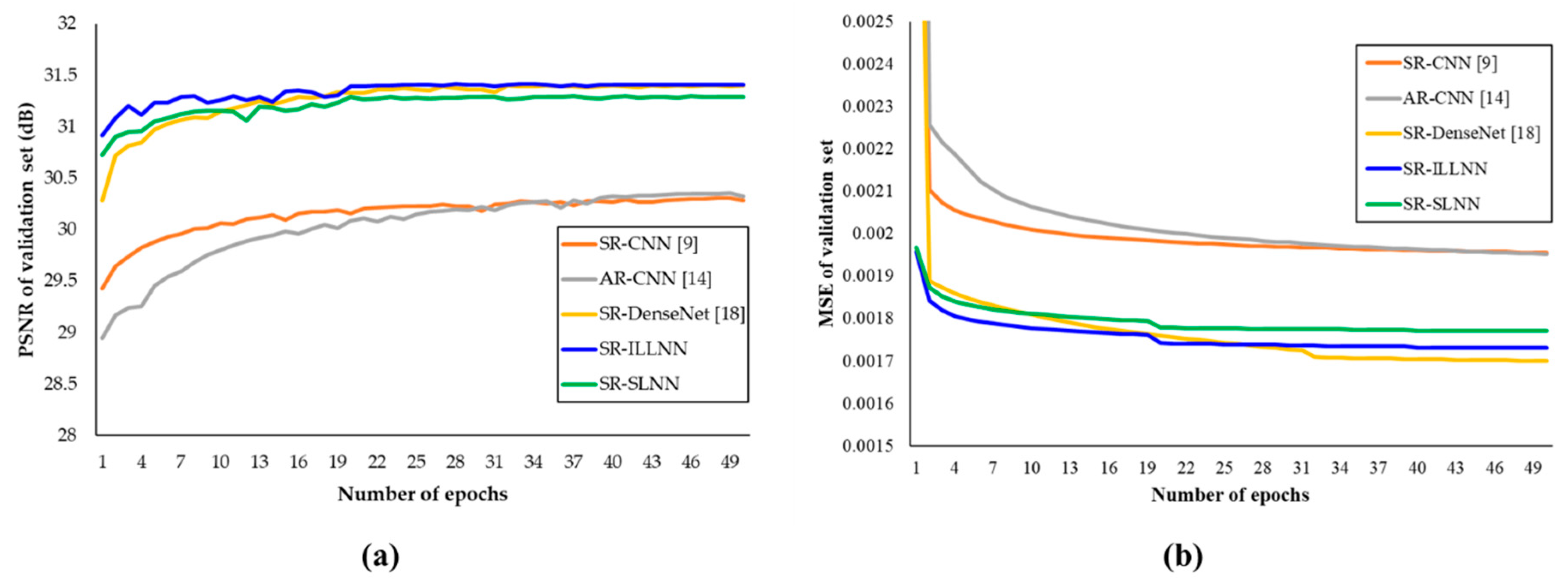
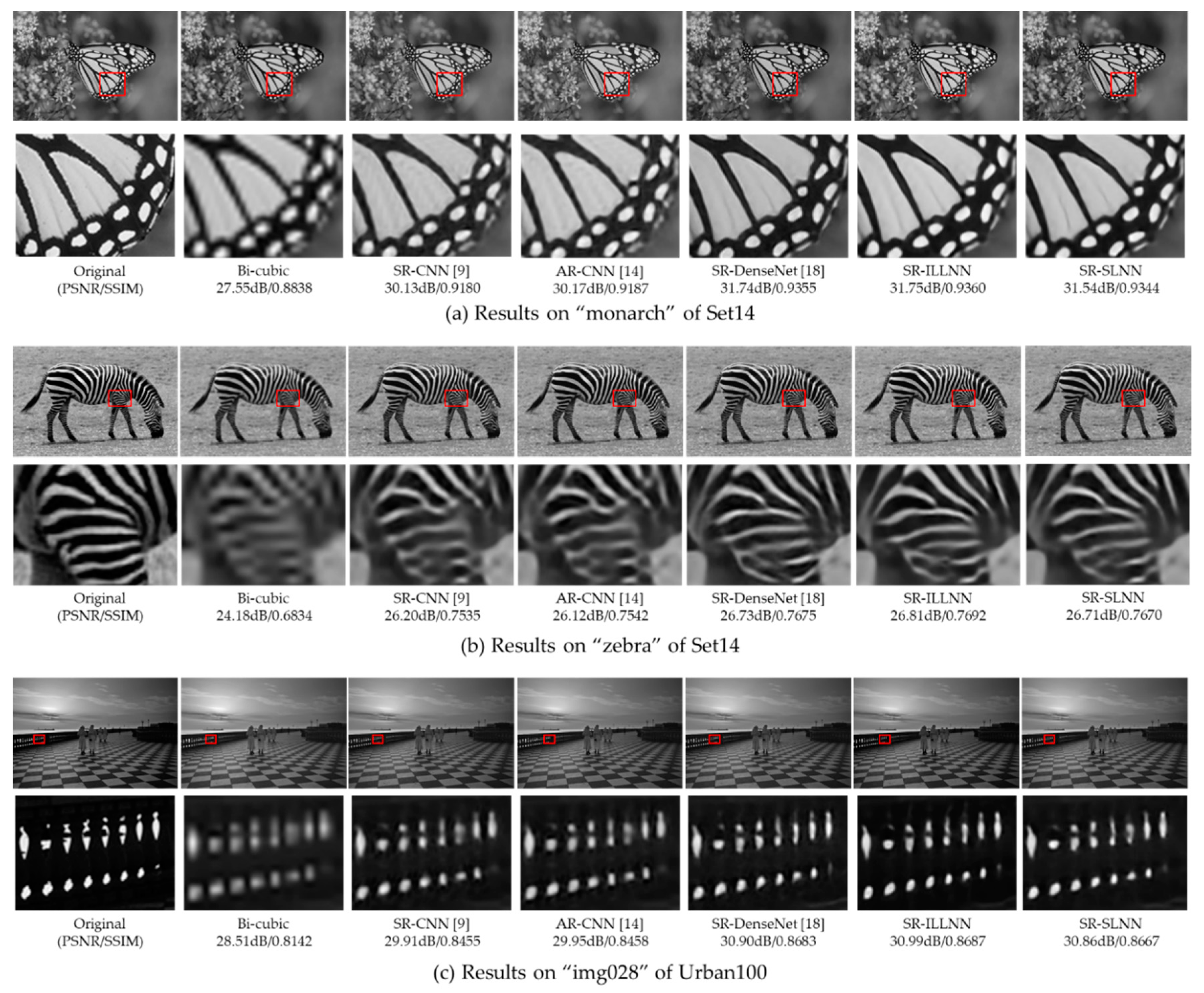
4. Experimental Results

As shown in Figure 4, we used the DIVerse 2K (DIV2K) dataset [24] whose total number is 800 images to train the proposed methods. In order to design SR-LNN capable of up-sampling input images four times, all training images with RGB components are converted into YUV components and extracted only Y component with the size of 100 × 100 patch without overlap. In order to generate interpolated input images, the patches are down-sampled and then up-sampled it again by bi-cubic interpolation.
Finally, we obtained three training datasets from DIV2K where the total number of each training dataset is 210,048 images for original images, low-resolution images, and interpolated low-resolution images, respectively. For testing our SR-LNN models, we used Set5, Set14, Berkeley Segmentation Dataset 100 (BSD100), and Urban100 as depicted in Figure 5, which are representatively used as testing datasets in most SR studies. For reference, Set5 was also used as a validation dataset.
All experiments were run on an Intel Xeon Skylake (eight cores @ 2.59 GHz) having 128 GB RAM and two NVIDIA Tesla V100 GPUs under the experimental environment described in Table 5. After setting a bicubic interpolation method as an anchor for performance comparison, we compared the proposed two SR-LNN models with SR-CNN [9], AR-CNN [14], and SR-DenseNet [18] in terms of image quality enhancement and network complexity.
In order to evaluate the accuracy of SR, we used PSNR and the structural similarity index measure (SSIM) [25,26] on the Y component as shown in Table 6 and Table 7, respectively. In general, PSNR has been commonly used as a fidelity measurement and it is the ratio between the maximum possible power of an original signal and the power of corrupting noise that affects the fidelity of its representation. In addition, SSIM is a measurement that calculates a score using structural information of images and is evaluated as similar to human perceptual scores. Compared with the anchor, the proposed SR-ILLNN and SR-SLNN enhance PSNR by as many as 1.81 decibel (dB) and 1.71 dB, respectively. Similarly, the proposed SR-LNNs show significant PSNR enhancement, compared to SR-CNN and AR-CNN. In contrast to the results of the anchor, the proposed SR-ILLNN has similar PSNR performance on most test datasets, compared with SR-DenseNet.
In addition, we conducted an experiment to verify the effectiveness of skip connections and dense connections. In particular, the more dense connections are deployed in the between convolution layers, the more network parameters are required in the process of convolution operations. Table 8 shows the results of tool-off tests on the proposed methods. As both skip connections and dense connections contribute to improve PSNR in the test datasets, the proposed methods are deployed these schemes. Figure 6 shows MSE as well as PSNR corresponding to the number of epochs and these experiments were evaluated from all comparison methods (SR-CNN, AR-CNN, and SR-DenseNet), including the proposed methods. It is confirmed that although SR-DenseNet has the highest reduction-rate in terms of MSE, the proposed methods have an almost similar increase rate in terms of PSNR. Figure 7 shows the comparisons of subjective quality between the proposed methods and previous methods.
In terms of the network complexity, we analyzed the number of parameters, parameter size (MB), and total memory size (MB) where total memory size includes intermediate feature maps as well as the parameter size. In general, both the total memory size and the inference speed are proportional to the number of parameters. Table 9 presents the number of parameters and total memory size. Compared with SR-DenseNet, the proposed two SR-LNNs reduce the number of parameters by as low as 8.1% and 4.8%, respectively. Similarly, the proposed two SR-LNNs reduce total memory size by as low as 35.9% and 16.1%, respectively. In addition, we evaluated the inference speed on BSD100 test images. As shown in Figure 8, the inference speed of the proposed methods is much faster than that of SR-DenseNet. Even though the proposed SR-SLNN is slower than SR-CNN and AR-CNN, it is obviously superior to SR-CNN and AR-CNN in terms of PSNR improvements as measured in Table 6 and Table 7.

5. Conclusions and Future Work

In this paper, we have proposed two SR-based lightweight neural networks (SR-ILLNN and SR-SLNN) for single image super-resolution. We investigated the trade-offs between the accuracy of SR (PSNR and SSIM) and the network complexity, such as the number of parameters, memory capacity, and inference speed. Firstly, SR-ILLNN was trained on both low-resolution and high-resolution images. Secondly, SR-SLNN was designed to reduce the network complexity of SR-ILLNN. For training the proposed SR-LNNs, we used the DIV2K image dataset and evaluated both the accuracy of SR and the network complexity on Set5, Set14, BSD100, and Urban100 test image datasets. Our experimental results show that the SR-ILLNN and SR-SLNN can significantly reduce the number of parameters by 8.1% and 4.8%, respectively, while maintaining similar image quality compared to the previous methods. As future work, we plan to extend the proposed SR-LNNs to other color components as well as a luminance component for improving SR performance on color images.

Author Contributions

Conceptualization, S.K. and D.J.; methodology, S.K. and D.J.; software, S.K.; validation, D.J., B.-G.K., H.L, and E.R.; formal analysis, S.K. and D.J.; investigation, S.K. and D.J; resources, D.J.; data curation, S.K.; writing—original draft preparation, S.K.; Writing—Review and editing, D.J.; visualization, S.K.; supervision, D.J.; project administration, D.J.; funding acquisition, H.L. and E.R. All authors have read and agreed to the published version of the manuscript.

Funding

This research was funded by Ministry of Science and ICT(MSIT) of the Korea government, grant number20PQWO-B153369-02.

Institutional Review Board Statement

Not applicable.

Informed Consent Statement

Not applicable.

Data Availability Statement

Not applicable.

Acknowledgments

This research was supported by a grant (20PQWO-B153369-02) from Smart road lighting platform development and empirical study on testbed Program funded by Ministry of Science and ICT(MSIT) of the Korea government. This research was results of a study on the “HPC Support” Project, supported by the ‘Ministry of Science and ICT’ and NIPA.

Conflicts of Interest

The authors declare no conflict of interest.

References

  1. Yang, W.; Zhang, X.; Tian, Y.; Wang, W.; Xue, J.; Liao, Q. Deep Learning for Single Image Super-Resolution: A Brief Review. IEEE Trans. Multimed. 2019, 21, 3106–3121. [Google Scholar] [CrossRef] [Green Version]
  2. Anwar, S.; Khan, S.; Barnes, N. A deep journey into super-resolution: A survey. arXiv 2019, arXiv:1904.07523. [Google Scholar] [CrossRef]
  3. Wang, Z.; Chen, J.; Hoi, S.C.H. Deep Learning for Image Super-resolution: A Survey. IEEE Trans. Pattern. Anal. Mach. Intell. 2020. [Google Scholar] [CrossRef] [PubMed] [Green Version]
  4. Keys, R. Cubic convolution interpolation for digital image processing. IEEE Trans. Acoust. 1981, 29, 1153–1160. [Google Scholar] [CrossRef] [Green Version]
  5. Freeman, T.; Jones, R.; Pasztor, C. Example-based super-resolution. IEEE Comput. Graph. Appl. 2002, 22, 56–65. [Google Scholar] [CrossRef] [Green Version]
  6. Kim, J.; Kim, B.; Roy, P.; Partha, P.; Jeong, D. Efficient facial expression recognition algorithm based on hierarchical deep neural network structure. IEEE Access 2019, 7, 41273–41285. [Google Scholar] [CrossRef]
  7. Kim, J.; Hong, G.; Kim, B.; Dogra, D. deepGesture: Deep learning-based gesture recognition scheme using motion sensors. Displays 2018, 55, 38–45. [Google Scholar] [CrossRef]
  8. Jeong, D.; Kim, B.; Dong, S. Deep Joint Spatiotemporal Network (DJSTN) for Efficient Facial Expression Recognition. Sensors 2020, 20, 1936. [Google Scholar] [CrossRef] [PubMed] [Green Version]
  9. Dong, C.; Loy, C.C.; He, K.; Tang, X. Image super-resolution using deep convolutional networks. IEEE Trans. Pattern. Anal. Mach. Intell. 2015, 38, 295–307. [Google Scholar] [CrossRef] [PubMed] [Green Version]
  10. Simonyan, K.; Zisserman, A. Very deep convolution networks for large -scale image recognition. In Proceedings of the International Conference on Learning Representations, San Diego, CA, USA, 7–9 May 2015. [Google Scholar]
  11. He, K.; Zhang, X.; Ren, S.; Sun, J. Deep residual learning for image recognition. In Proceedings of the Conference on Computer Vision and Pattern Recognition, Las Vegas, NY, USA, 27–30 June 2016; pp. 770–778. [Google Scholar]
  12. Huang, G.; Liu, Z.; Van Der Maaten, L.; Weinberger, K.Q. Densely connected convolutional networks. In Proceedings of the Conference on Computer Vision and Pattern Recognition, Honolulu, HI, USA, 21–26 July 2017; pp. 4700–4708. [Google Scholar]
  13. Ioffe, S.; Szegedy, C. Batch normalization: Accelerating deep network training by reducing internal covariate shift. In Proceedings of the Machine Learning Research, Lille, France, 7–9 July 2015; pp. 448–456. [Google Scholar]
  14. Dong, C.; Deng, Y.; Change Loy, C.; Tang, X. Compression artifacts reduction by a deep convolutional network. In Proceedings of the International Conference on Computer Vision, Santiago, Chile, 7–13 December 2015; pp. 576–584. [Google Scholar]
  15. Kim, J.; Lee, J.; Lee, K. Accurate image super-resolution using very deep convolutional networks. In Proceedings of the Conference on Computer Vision and Pattern Recognition, Las Vegas, NY, USA, 27–30 June 2016; pp. 1646–1654. [Google Scholar]
  16. Ledig, C.; Theis, L.; Huszár, F.; Caballero, J.; Cunningham, A.; Acosta, A.; Aitken, A.; Tejani, A.; Totz, J.; Wang, Z.; et al. Photo-realistic single image super-resolution using a generative adversarial network. In Proceedings of the Conference on Computer Vision and Pattern Recognition, Honolulu, HI, USA, 21–26 July 2017; pp. 4681–4690. [Google Scholar]
  17. Lim, B.; Son, S.; Kim, H.; Nah, S.; Lee, K. Enhanced deep residual networks for single image super-resolution. In Proceedings of the Conference on Computer Vision and Pattern Recognition Workshops, Honolulu, HI, USA, 21–26 July 2017; pp. 136–144. [Google Scholar]
  18. Tong, T.; Li, G.; Liu, X.; Gao, Q. Image super-resolution using dense skip connections. In Proceedings of the Conference on Computer Vision and Pattern Recognition, Honolulu, HI, USA, 21–26 July 2017; pp. 4799–4807. [Google Scholar]
  19. Ye, Y.; Alshina, E.; Chen, J.; Liu, S.; Pfaff, J.; Wang, S. [DNNVC] AhG on Deep neural networks based video coding, Joint Video Experts Team (JVET) of ITU-T SG 16 WP 3 and ISO/IEC JTC 1/SC29, Document JVET-T0121, Input Document to JVET Teleconference. 2020.
  20. Cho, S.; Lee, J.; Kim, J.; Kim, Y.; Kim, D.; Chung, J.; Jung, S. Low Bit-rate Image Compression based on Post-processing with Grouped Residual Dense Network. In Proceedings of the Conference on Computer Vision and Pattern Recognition Workshops, Long Beach, CA, USA, 16–20 June 2019. [Google Scholar]
  21. Yang, R.; Xu, M.; Liu, T.; Wang, Z.; Guan, Z. Enhancing quality for HEVC compressed videos. IEEE Trans. Circuits Syst. Video Technol. 2018, 29, 2039–2054. [Google Scholar] [CrossRef] [Green Version]
  22. Zhang, S.; Fan, Z.; Ling, N.; Jiang, M. Recursive Residual Convolutional Neural Network-Based In-Loop Filtering for Intra Frames. IEEE Trans. Circuits Syst. Video Technol. 2019, 30, 1888–1900. [Google Scholar] [CrossRef]
  23. Lui, G.; Shih, K.; Wang, T.; Reda, F.; Sapra, K.; Yu, Z.; Tao, A.; Catanzaro, B. Partial convolution based padding. arXiv 2018, arXiv:1811.11718. [Google Scholar]
  24. Agustsson, E.; Timofte, R. NTIRE 2017 Challenge on Single Image Super-Resolution: Dataset and Study. In Proceedings of the Conference on Computer Vision and Pattern Recognition Workshops, Honolulu, HI, USA, 21–26 July 2017. [Google Scholar]
  25. Wang, Z.; Bovik, A.C.; Sheikh, H.R.; Simoncelli, E.P. Image quality assessment: From error visibility to structural similarity. IEEE Trans. Image Processing 2004, 13, 600–612. [Google Scholar] [CrossRef] [PubMed] [Green Version]
  26. Yang, C.; Ma, C.; Yang, M. Single-image super-resolution: A benchmark. In Proceedings of the European Conference on Computer Vision, Zurich, Switzerland, 6–12 September 2014; pp. 372–386. [Google Scholar]
Figure 1. The framework of SR-DenseNet [18].
Applsci 11 01092 g001
Figure 2. The framework of the proposed SR-ILLNN.
Applsci 11 01092 g002
Figure 3. The framework of the proposed SR-SLNN.
Applsci 11 01092 g003
Figure 4. Training dataset. (DIV2K).
Applsci 11 01092 g004
Figure 5. Test datasets. (Set5, Set14, BSD100, and Urban100).
Applsci 11 01092 g005
Figure 6. PSNR and MSE corresponding to the number of epochs. (a) PSNR per epoch. (b) MSE per epoch.
Applsci 11 01092 g006
Figure 7. Comparisons of subjective quality on test dataset. (a) Results on “monarch” of Set14. (b) Results on “zebra” of Set14. (c) Results on “img028” of Urban100.
Applsci 11 01092 g007
Figure 8. Inference speed on BSD100.
Applsci 11 01092 g008
Table 1. Analysis of network parameters in SR-ILLNN.
Layer
Name
Kernel
Size
Num. of
Kernels
Padding
Size
Output Feature Map
(W × H × C)
Num. of
Parameters
Conv13 × 3 × 1641N × M × 64640
Conv23 × 3 × 64641N × M × 6436,928
Conv33 × 3 × 128641N × M × 6473,792
Conv43 × 3 × 192641N × M × 64110,656
Conv51 × 1 × 64320N × M × 322080
Deconv14 × 4 × 323212N × 2M × 3216,416
Conv6, 73 × 3 × 323212N × 2M × 329248
Deconv24 × 4 × 323214N × 4M × 3216,416
Conv83 × 3 × 321614N × 4M × 164624
Conv95 × 5 × 16424N × 4M × 641664
Conv103 × 3 × 646414N × 4M × 6436,928
Conv113 × 3 × 1286414N × 4M × 6473,792
Conv123 × 3 × 1921614N × 4M × 1627,664
Conv13, 143 × 3 × 323214N × 4M × 329248
Conv155 × 5 × 32124N × 4M × 1801
Table 2. Analysis of network parameters in SR-SLNN.
Layer
Name
Kernel
Size
Num. of
Kernels
Padding
Size
Output Feature Map
(W × H × C)
Num. of
Parameters
Conv15 × 5 × 1642N × M × 641664
Conv23 × 3 × 64641N × M × 6436,928
Conv33 × 3 × 128641N × M × 6473,792
Conv43 × 3 × 192641N × M × 64110,656
Conv51 × 1 × 64320N × M × 322080
Deconv14 × 4 × 323212N × 2M × 3216,416
Deconv24 × 4 × 323214N × 4M × 3216,416
Conv63 × 3 × 321614N × 4M × 164624
Conv75 × 5 × 16124N × 4M × 1401
Table 3. Hyper-parameters of the proposed methods.
OptimizerAdam
Learning Rate10−3 to 10−5
Activation functionReLU
Padding ModePartial convolutional based padding [23]
Num. of epochs50
Batch size128
Initial weightXavier
Table 4. Relation between the number of parameters and PSNR according to the various filter sizes.
NetworksFilter Size
(Width × Height)
Num. of
Parameters
PSNR
(dB)
SR-ILLNN3 × 3439,39331.41
5 × 51,153,12131.38
7 × 72,223,71331.29
9 × 93,651,16928.44
SR-SLNN3 × 3262,97731.29
5 × 5664,38531.19
7 × 71,266,49731.16
9 × 92,069,31331.15
Table 5. Experimental environments.
Num. of Training Samples210,048
Input size (XLR)25 × 25 × 1
Interpolated input size (XILR)100 × 100 × 1
Label size (YHR)100 × 100 × 1
Linux versionUbuntu 16.04
CUDA version10.1
Deep learning frameworksPytorch 1.4.0
Table 6. Average results of PSNR (dB) on the test dataset.
DatasetBicubicSR-CNN [9]AR-CNN [14]SR-DenseNet [18]SR-ILLNNSR-SLNN
Set528.4430.3030.3531.4331.4131.29
Set1425.8027.0927.1027.8427.8327.73
BSD10025.9926.8626.8627.3427.3327.28
Urban10023.1424.3324.3425.3025.3225.18
Average24.7325.8025.8126.5326.5426.44
Table 7. Average results of SSIM on the test dataset.
DatasetBicubicSR-CNN [9]AR-CNN [14]SR-DenseNet [18]SR-ILLNNSR-SLNN
Set50.81120.85990.86140.88440.88480.8827
Set140.70330.74950.75110.77080.77090.7689
BSD1000.66990.71120.71260.72790.72750.7260
Urban1000.65890.71580.71770.75840.75830.7532
Average0.67020.71920.72080.74810.74790.7447
Table 8. The results of tool-off tests.
Skip
Connections
Dense
Connections
Set5 (PSNR)Set14 (PSNR)BSD100 (PSNR)Urban100 (PSNR)
SR-ILLNNSR-SLNNSR-ILLNNSR-SLNNSR-ILLNNSR-SLNNSR-ILLNNSR-SLNN
DisableDisable31.3431.1527.8027.6227.3127.2025.2725.01
EnableDisable31.3531.2127.8127.6827.3327.2625.3125.13
DisableEnable31.4031.1827.8127.6527.3227.2325.2925.07
EnableEnable31.4131.2927.8327.7327.3327.2825.3225.18
Table 9. Analysis of the number of parameters and memory size.
SR-CNN [9]AR-CNN [14]SR-DenseNet [18]SR-ILLNNSR-SLNN
Num. of parameters57,281106,5645,452,449439,393262,977
Parameter size (MB)0.220.4120.801.681.00
Total memory size (MB)14.9817.61224.8180.8336.21
Publisher’s Note: MDPI stays neutral with regard to jurisdictional claims in published maps and institutional affiliations.

