Article

WAMs Based Eigenvalue Space Model for High Impedance Fault Detection

Department of Electrical and Computer Engineering, University of Florida, Gainesville, FL 32611-6200, USA
*
Author to whom correspondence should be addressed.
Appl. Sci. 2021, 11(24), 12148; https://doi.org/10.3390/app112412148
Submission received: 6 November 2021 / Revised: 3 December 2021 / Accepted: 13 December 2021 / Published: 20 December 2021
(This article belongs to the Special Issue Intelligent Fault Diagnosis of Power System)

Abstract

:
High impedance faults present unique challenges for power system protection engineers. The first challenge is the detection of the fault, given the low current magnitudes. The second challenge is to locate the fault to allow corrective measures to be taken. Corrective actions are essential as they mitigate safety hazards and equipment damage. The problem of high impedance fault detection and location is not a new one, and despite the safety and reliability implications, relatively few efforts have been made to find a general solution. This work presents a hybrid data driven and analytical-based model for high impedance fault detection in distribution systems. The first step is to estimate a state space model of the power line being monitored. From the state space model, eigenvalues are calculated, and their dynamic behavior is used to develop zones of protection. These zones of protection are generated analytically using machine learning tools. High impedance faults are detected as they drive the eigenvalues outside of their zones. A metric called eigenvalue drift coefficient was formulated in this work to facilitate the generalization of this solution. The performance of this technique is evaluated through case studies based on the IEEE 5-Bus system modeled in Matlab. Test results are encouraging indicating potential for real-life applications.

1. Introduction

High impedance faults in electric power systems (EPS) represent a liability in regards to safety and reliability. High impedance faults (HIFs) arise when a connection is made between an energized conductor and a surface with high resistance that is not part of the EPS. Common surfaces that can lead to HIFs include trees, asphalt, concrete, sand, and grass [1]. Significant damage to equipment, property, and even fatalities have been attributed to this phenomenon [2]. Despite these significant implications, the problem of HIFs remains unsolved [3]. One of the main challenges in this area is presented by the unique nature of HIFs [4]: The nonlinear relationship between currents and voltages, the presence of electrical arcs, and most importantly the low current magnitudes. These characteristics make it difficult to detect HIF by the traditional means of over-current protection. A protection device on a heavily loaded feeder will most likely not operate in the presence of HIFs. On the other hand, choosing to set a protective device too close to the expected loading level can lead to nuisance tripping. To compound the problem even further, the dynamic behavior of both the fault and the load must be taken into account.
As a result of the clear limitations of over-current protection in the detection of HIFs, efforts have been made to find alternate solutions to this problem. Several techniques have been proposed in recent years, but a unified and general solution is yet to be accepted by the industry [5]. Most techniques can be divided into the following groups: knowledge-based techniques, network topology based techniques, and apparent impedance-based techniques.
Knowledge-based techniques leverage data acquired by meters and utilize machine learning (ML) approaches to identify outliers [6]. One of the drawbacks of these techniques is the reliance on meters, and the infrastructure necessary to process large amounts of data.
Methods based on network topology are somewhat similar to knowledge-based solutions in that they rely on metering [7]. Meter sensors in key areas are deployed to create a network capable of detecting HIFs. This approach requires a significant investment in terms of equipment, installation and maintenance of meters. Moreover, this type of approach suffers from a lack of generality, which means that significant engineering is needed in real-life applications.
Transmission protection techniques have inspired researchers to develop solutions for HIFs based on methods such as Apparent Impedance. These techniques are appealing due to the relatively low investment cost and the familiarity of protection engineers with the underlying principle of impedance (distance) relaying. A significant obstacle these techniques face is the stochastic behavior of HIFs. Several of these solutions make the assumption that the impedance at the fault point is purely resistive, which would lead to a fault signature that is fairly linear and constant [8]. These techniques were advanced by taking into account the non-linear behavior of an electrical arc. These models face two challenges: Being able to detect the change in impedance, and doing so in small time windows. Still, despite having multiple unresolved issues, impedance-based techniques have gone on to become accepted as the framework for the development of new HIF detection and location solutions [9].
Solutions based on state estimators, such Weighted Least Squares (WLS) [10,11], have been proposed more recently. These solutions aim to detect HIFs by identifying statistical outliers during the estimation process. Estimation-based methods such as [12] have been proposed in the time domain, as well as in the frequency domain as presented in [8,13]. In regards to state estimators for HIFs, frequency domain techniques appear to have greater momentum compared to time domain approaches due to reported advantages such as noise suppression and relative ease of implementation. Despite encouraging results produced by Frequency Domain Estimators, several limitations of this approach must be noted: First, there is a lack of a generalized solution, particularly in regards to the system’s topology, and secondly, the estimation of system parameters, including the fault itself, has not been standardized. Some of the solutions based on frequency domain estimators attempt to streamline the process by modeling and estimating a reduced number of parameters, which leads to marginal observability and near singular Jacobian matrices. Both of these lead to reduced redundancy and a possible magnification of errors [1,14]. Another important limitation of WSL estimators to be considered is that the vast majority of them only consider the residual of the error, which does not always represent the total error [15,16].
An approach based on neural networks is used in [17], which derives estimates of the parameters of a feeder during fault conditions. The estimation is carried out in the time domain, and utilizes polynomial approximation techniques. This approach is hindered by assumptions related to the time-frame when measurements are taken and the location of the load [18].
Recently, in [19], the harmonic distortion generated during the fault is analyzed in the spectral domain. This solution detects HIFs by identifying parameter errors in the fundamental and the third harmonic through a WLS estimator. This technique yields a high rate of detection and an accurate location of the fault, however, implementation presents serious challenges as some of the parameters required to solve the estimator must be calculated manually.
Finally, solutions based on WAMs technology were utilized by studies in [20,21,22]. In [20], a Fourier Series based approach is proposed in which parameters are estimated from harmonics measured by PMUs. This approach is similar to other frequency domain approaches, and although the idea seems promising, implementation could be an issue due to short windows of time when measurements must be made, and the use of specialized measurements and parameters that could lead to singular matrices. It must also be noted that [20] was not evaluated in a recognized environment such as an I E E E Test Feeder. In [21], a combination of measurements and simulations are used to locate faults. As mentioned before, the need to simulate parameters leads to solutions that are not general and can be difficult to implement. In [22], measurements from multiple sections of a line are utilized to derive a model based on symmetrical components with emphasis on line capacitance to detect and locate faults. The results were interesting; however, it was noted that the performance of the algorithm is affected by the length of the line, and the solution was not tested with resistances beyond 100 Ω . Moreover, this solution appears to be geared towards systems with underground cables.
This review of the literature has lead to the following conclusions:
  • Most acceptable solutions are based on the Apparent Impedance framework.
  • The Time Domain vs. Frequency Domain debate is still open.
  • Most solutions focus on modeling and identifying specific aspects of HIFs.
  • Most solutions suffer from a lack of generality, meaning that manual adjustments have to be made each time the solution is deployed.
In view of the limitations of existing solutions and the current state of smart grid technology, this work presents a unified, dynamic hybrid data-driven and analytical-based model, which advances the state-of-the-art of HIFs detection in the following ways:
  • Presents a data-driven and analytical model, based on novel statistical metrics, for the identification of eigenvalue drift patterns.
  • Temporal characteristics of a real-life power system are modeled through autonomously generated protection zones in the eigenvalue space.
The remainder of this paper is organized as follows. Section 2 provides theoretical background on state estimation, clustering techniques, power system protection, and eigenvalue properties. Section 3 presents the unified model with the accompanying metrics formulated for this work. Test results of a case study are shown in Section 4. Finally, Section 5 presents conclusions and remarks on the future direction of this work.

2. Background Information

2.1. State Space Representation

Mathematical tools such as differential equations make it possible to model the behavior of physical systems. Once these equations have been derived, multiple techniques such as transformations can be applied to refine the model. Transformations can be used to take the mathematical model of a system from one domain into another in order to unveil a desired characteristic. A system can also be represented in a way that highlights a desired feature or relationship. One particular model which emphasizes the relationship between the input (stimuli) and the output (the observable behavior) is the State Space representation [23]:
x ˙ = A x + B u
y = C x + D u
where the state vector x, contains a set of state variables. State variables provide information about the system, which makes it possible to estimate a transition from the current state into a future state. y is the output vector that represent the linear combination of observable behavior of the system. u is a vector that contains the set of inputs or stimuli that drive the behavior of the states. A and B are constant matrices that define the relationship between the input and the state variables. C and D are constant matrices that define the relationship between the state variables and input with the output. Matrix A is particularly important for this work, as it is the matrix that is used to estimate the eigenvalues of the system.
State Space was chosen for this work as it facilitates system estimation in the presence of multiple inputs and outputs, and doesn’t require the initial conditions of the system to be known, which seldom is the case when estimating an operational power system. Finally state space simplifies the process of generalization as all systems of the same type and order will have the same State Space structure.
Many techniques have been developed for dynamic state state estimation, most of them are based on the Kalman Filter [23,24,25]. Subspace estimation, used in this work, is now introduced.

2.2. Subspace Estimation

Multiple techniques can be used to estimate the eigenvalues of a system. These techniques include approximate realizations and subspace identification. A linear time invariant approximate realization aims to derive a minimum order model using the impulse response of the system through Markov Parameters as follows. Starting with a State Space model [23]:
x ( k + 1 ) = A x ( k ) + B u ( k )
y ( k ) = C x ( k ) + D u ( k )
which has a transfer function
G ( z ) = k = 0 g ( k ) z k
where g ( k ) is a known impulse response for
k = 0 , 1 , ,
The state matrices and the transfer function share the following relationship:
G ( z ) = D + C ( z I A ) 1 B
The matrices can be computed from the impulse as follows,
g ( k ) = D for k = 0 C A k 1 B for k 1
The Ho-Kalman algorithm is applied to find matrices A, B, and C through the Hankel matrix H
H n r , n c = g ( 1 ) g ( 2 ) g ( 3 ) g ( n c ) g ( 2 ) g ( 3 ) g ( 4 ) g ( n c + 1 ) g ( 3 ) g ( 4 ) g ( 5 ) g ( n c + 2 ) g ( n r ) g ( n r + 1 ) g ( n r + 2 ) g ( n r + n c 1 )
The Hankel matrix can be represented in the following form:
H n r , n c = C C A C A n r 1 B A B A n c 1 B
The rank n of the Hankel matrix is equal to the rank of matrix A. Singular Value decomposition is used to determine the rank of the Hankel matrix as follows:
H = U n Σ n V n T
where U n and V n are unitary matrices
U n T U n = V n T V n = I n
Σ n is a diagonal matrix with positive singular values on the diagonal. The number of non-zero singular values across the diagonal of the matrix is equivalent to the rank of the Hankel matrix, which is also, as discussed previously, the rank of A.
The Hankel matrix can then be expressed as
H = U n Σ n 1 / 2 Σ n 1 / 2 V n T
where Σ n 1 / 2 represents a diagonal matrix composed of the square roots of the singular values. Matrix B is the first column of Σ n 1 / 2 V n T , while C is the first row of U n Σ n 1 / 2 .
Finally, A can be defined as
A = Σ n 1 / 2 U n T H V n Σ n 1 / 2
where H represents the shifted Hankel matrix
H n r , n c = g ( 1 ) g ( 2 ) g ( 3 ) g ( n c ) g ( 2 ) g ( 3 ) g ( 4 ) g ( n c + 1 ) g ( 3 ) g ( 4 ) g ( 5 ) g ( n c + 2 ) g ( n r ) g ( n r + 1 ) g ( n r + 2 ) g ( n r + n c 1 )
A limitation of the Approximate Realization approach is that system parameters are estimated from the response of the system to an impulse. In real-life, at least in the context of power systems, this is not practical. As a result, alternative methods that use information from the system’s inputs and outputs to achieve similar results have been developed. In subspace identification the State Space model of the system can be expressed in the innovation form as [23]:
x k + 1 = A x k + B u k + K e k
y k = C x k + D u k + e k
where u k represents the input vector, and is y k the output. e k represents a source of noise and K contains parameters of the noise model.
The output can be defined as
y k = G ( z ) u k + H ( z ) e k
where
G ( z ) = C ( z I A ) 1 B + D
and
H ( z ) = C ( z I A ) 1 K + I
A key part of this estimation procedure is the derivation of the Observability matrix:
O = C C A C A r 1
Once again Singular Value Decomposition can be used to find the rank of the Observability matrix, which is also the rank of the A matrix. Applying linear regression techniques to the relationships described above the matrices A, B, C, D, noise components, and initial states can be estimated [23].

2.3. Eigenvalue Space

As previously mentioned, one of the advantages of the State Space representation is that it offers inherent access to the eigenvalues of a system. In the context of this work, the eigenvalues represent the frequencies of oscillation of a system, which can be represented as complex numbers. These eigenvalues evolve overtime and thus provide an estimation of the system’s operating condition. In this work, the impedance of the transmission line is referred to as the system, and the eigenvalues are the frequencies of oscillation of the powerline. This work takes advantage of the unique nature of the eigenvalues of a system. One can think of eigenvalues as the finger-prints of the system, a unique identifier arising from a combination of resistance, capacitance, and inductance seen across the system. The temporal characteristics of the eigenvalues are accounted for in this work, as they are estimated dynamically, and their drift over time is used to make decisions regarding the status of the system. Eigenvalues are mapped into a space this works refers to as the Eigenvalue Space, which is based on the Cartesian Coordinate System. This is done to avoid complications related to the handling of complex numbers.

2.4. Protection Schemes

Distance and Out-of-Step relaying schemes served in part as the basis for the development of the solution presented in the next section. These schemes are introduced briefly as follows: Distance relays utilize voltage and current measurements to estimate the impedance of a powerline. This resulting impedance is graphed in the X-R plane, and is usually accompanied by a circle. The diameter and location of this circle with respect to the axis are predetermined for each line, and define the abnormal zones of operation for the power line [26]. When a fault occurs, the magnitude of the current increases bringing the impedance seen by the relay to an area inside the zone of protection. Once the impedance is inside the zone of protection, and after a pre-programmed delay, the relay makes a decision to initiate a trip sequence. Figure 1 illustrates the characteristics of a version of the Distance Relay, the Mho Relay.
Out-of-Step Relays distinguish acceptable operating conditions from potentially hazardous conditions by leveraging the spatial characteristics and rate of change of the system’s impedance. Zones of protection similar to those seen in distance relays are established in Out-of-Step Relays, but in addition to tracking the angle and magnitude of the impedance, the relay times impedance as it moves in the R-X plane. Decisions are made based on how far inside the zone of protection the impedance has traveled, and how long it has been there. Figure 2 illustrates the characteristics of an Out-of-Step Relay.

2.5. Clustering

The principles of protection discussed in the previous sub-section are used to estimate the region were the eigenvalues reside during normal operation. In order to accommodate the unique location and drift patterns of the eigenvalues of a line, eigenvalues are separated into clusters. In this work k-means clustering was utilized to develop the eigenvalue clusters [27].
The goal of k-means clustering is to find patterns or similarities among the members of a dataset. These patterns are then used to separate the data points into groups where the members share similar characteristics [28]. Typically, metrics such as the Squared Euclidean Distance are used as the basis of the algorithm. The Squared Euclidean Distance is expressed as a sum of squares:
d 2 ( p , q ) = ( p 1 q 1 ) 2 + ( p 2 q 2 ) 2 + + ( p n q n ) 2
where d is the distance between two points, while p and q are the coordinates of a point in the Euclidean Space. k-means clustering is an iterative algorithm, where the clusters are re-calculated and cluster members are reassigned to different clusters until a convergence criteria is met.

3. HIF Detection in Eigenvalue Space

Merely a decade ago, proposing a solution based on advanced metering at multiple ends of a line, with the end goal of estimating eigenvalues, would have been met with significant scepticism regarding the feasibility of the solution’s implementation. However, due to increased integration of synchrophasor technology into the grid, solutions based on Wide Area Measurements (WAMS) made possible by Phasor Measurement Units (PMUs) are gaining momentum. Even at the distribution level, smaller and cheaper units called Micro-PMUs are being added to the smart grid [24].
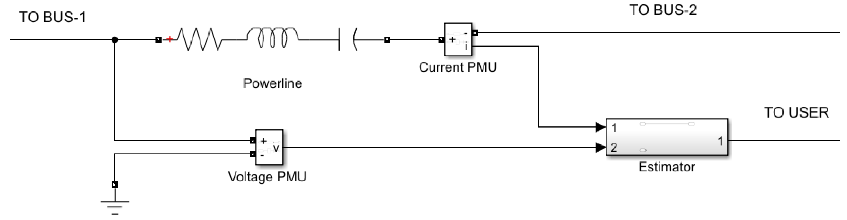
This work envisions PMUs, as the metering devices collecting information for the eigenvalue estimation step. This is due to their high sampling rates (120 Hz), and wide area measuring capabilities. These two characteristics are critical as higher sampling rates increase the robustness of the estimates, while the ability to operate over a wide area means that this solution could be implemented on lines of varying length. Figure 3 illustrates the configuration of the system proposed in this work.
One of the key features that distinguishes this work from other solutions is that this method doesn’t attempt to identify HIFs or their characteristics, but instead focuses on identifying deviations in the Eigenvalue Space (ES). Identifying HIFs by focusing on the characteristics of the fault presents an immense engineering challenge, but this is a challenge that can be avoided altogether.
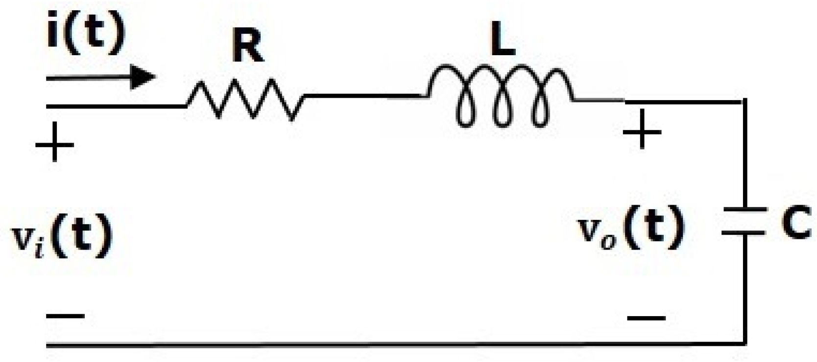
As mentioned in the previous section, each powerline has a unique set of eigenvalues determined by the parameters illustrated in Figure 4, and these eigenvalues are sensitive to changes in impedance, such as the deviations seen during a fault.
Therefore, instead of trying to predict the magnitude and order of the harmonics generated by an electrical arc, or how a highly resistive surface will change the angle of an apparent impedance, this works presents a method that establishes a baseline of acceptable values in the ES and makes decisions when eigenvalues drift outside of these zones. Focusing on deviations from a baseline allows this solution to:
  • Utilize alternative means of monitoring, in this case eigenvalues.
  • Create a significantly higher degree of generalization as the solution can applied to just about any system with virtually zero human interaction (other than the installation of the metering infrastructure).

3.1. Framework for Eigenvalue Identification

The first step of this solution is to estimate the eigenvalues of the powerline being monitored. Figure 5 is an example of the estimation result. Using PMUs, voltage readings from one end of the line can be integrated with current measurements at the opposite end of the line. These two measurements are then sent to an estimator. Physically, the estimator can reside at either a centralized location, such as a control center or database, or at a secure distributed location such as a substation. This versatility regarding the location of the equipment adds to the generality of the solution.
As discussed in the previous section, Subspace Estimation was used to realize the eigenvalues of the system, however, other algorithms can be used to process the data collected by the PMUs and estimate the eigenvalues. The choice of the estimation algorithm is not critical, as long as the output provided by the estimator is reliable and consistent. This work is not concerned with identifying the parameters of the system with great accuracy with respect to the real (physical) values. The algorithms used in this work establish a benchmark of acceptable operating regions in the Eigenvalue Space.

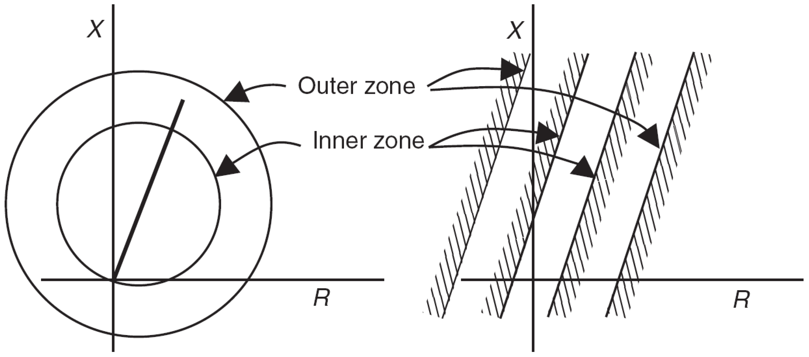
3.2. Framework for Zones of Protection in Eigenvalue Space

The output of the Subspace estimator is used to build eigenvalue clusters. These clusters are created using k-means clustering techniques. The clusters are dynamic, and can be updated at user specified intervals or whenever new data becomes available. In this work, simulated PMU readings collected over a 24-h period were used to train the clustering algorithm. The load profile, illustrated in Figure 6, was modeled after Houston, TX with data provided by ERCOT [29].
In order to facilitate the creation of the zones of protection and improve their reliability, statistical metrics are used to evaluate the suitability of the clusters. As part of this work a metric referred to as the Eigenvalue Drift Coefficient (EDC) was developed. After the clustering algorithm has converged, vectors containing the Euclidean distance between pairs of eigenvalues in each cluster are created. From this set of values, the mean distance and standard deviation within each cluster is computed. The EDC of each cluster is calculated as follows:
E D C = σ μ
where σ is the standard deviation, and μ is the mean of the distances.
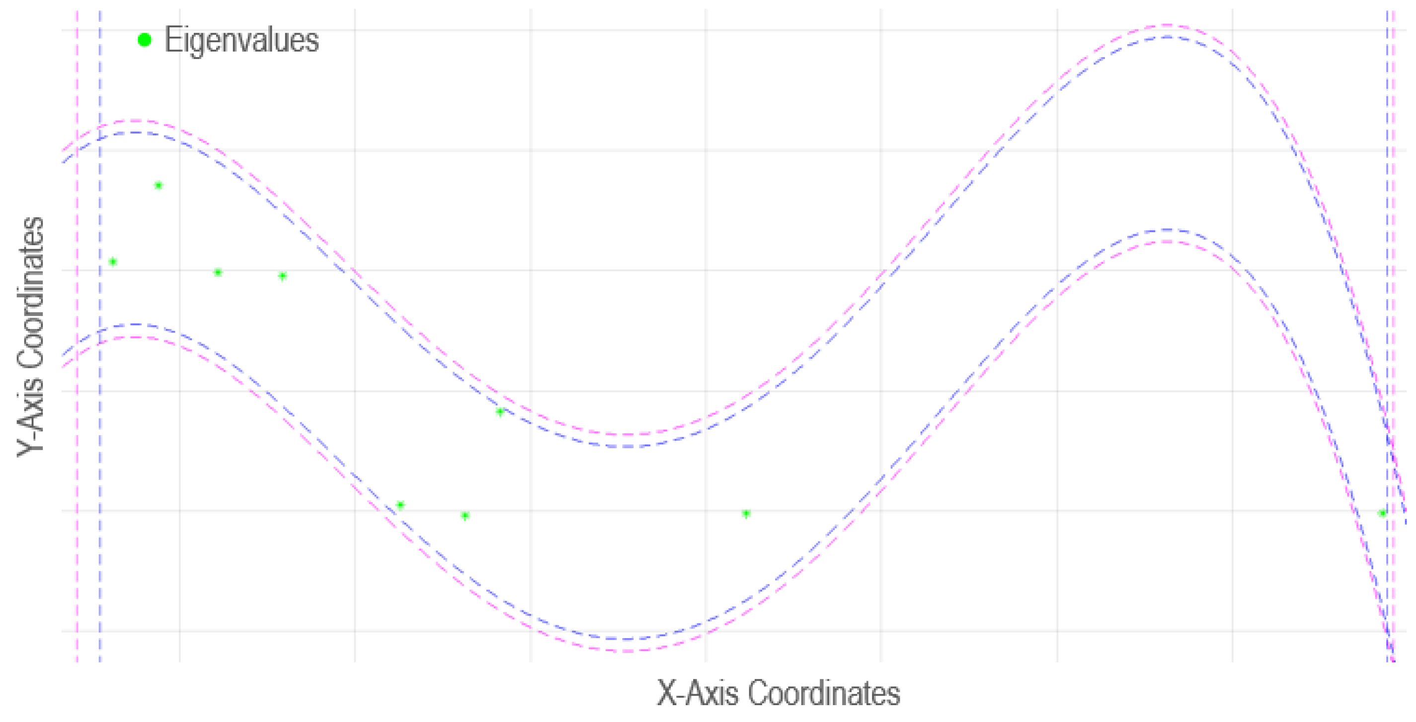
Clusters with a high EDC tend to have a relatively uniform distribution compared to clusters with a low EDC. Clusters with high EDC yield zones of protection which are more secure. The clustering step is repeated until all clusters produce acceptable EDC values. Polynomial curve fitting is then used to define the zones of protection. Low and high EDC clusters are illustrated in Figure 7 and Figure 8, respectively. High EDC values allow for the use of lower degree polynomials for curve fitting.
The number of clusters used by the algorithm is determined iteratively, starting with 6 clusters, and decreasing the number of clusters until EDCs higher than 1.7 are achieved for all clusters. At EDCs higher than 1.7, polynomials of degree 3 and less can be used to produce the zones of protection. For clusters with an EDC at or less 1.7, polynomials of degrees 3 and less might not provide a suitable fit. In addition to having to utilize higher degree polynomials for curve fitting, a low EDC also leads to protection zones where most of the eigenvalues are not at the center of the zone. Off-centered eigenvalues ultimately lead to zones with inconsistent safety margins, which could lead to false positives if eigenvalues near the edge of the zone drift outside during normal operation, or delayed reaction during an abnormal condition for eigenvalues located in a particularly wide area of the zone.
Safety margins are created using the mean μ of the cluster, and a multiplier corresponding to the magnitude of μ . For higher values of μ , the algorithm uses smaller multipliers, while higher multipliers are used for smaller values of μ . Two zones of protection are used for each cluster. An inner zone where the eigenvalues reside during normal operation, and an outer zone that generates an immediate reaction. If an eigenvalue drifts to the area in between the two zones, a timer is started. If the eigenvalue returns to the inner zone before the timer expires, no action is taken. However, if the eigenvalue doesn’t return to the inner zone before the time expires or continues to drift beyond the second zone, action is taken. For this work, a time period equivalent to the cluster update time was used.

3.3. High Impedance Fault Detection

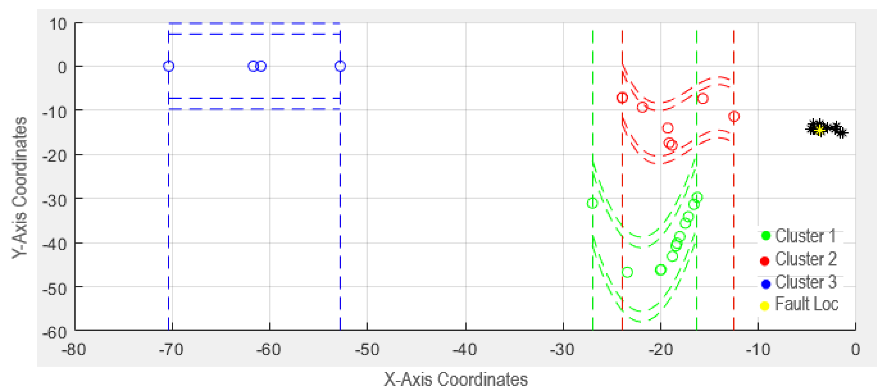
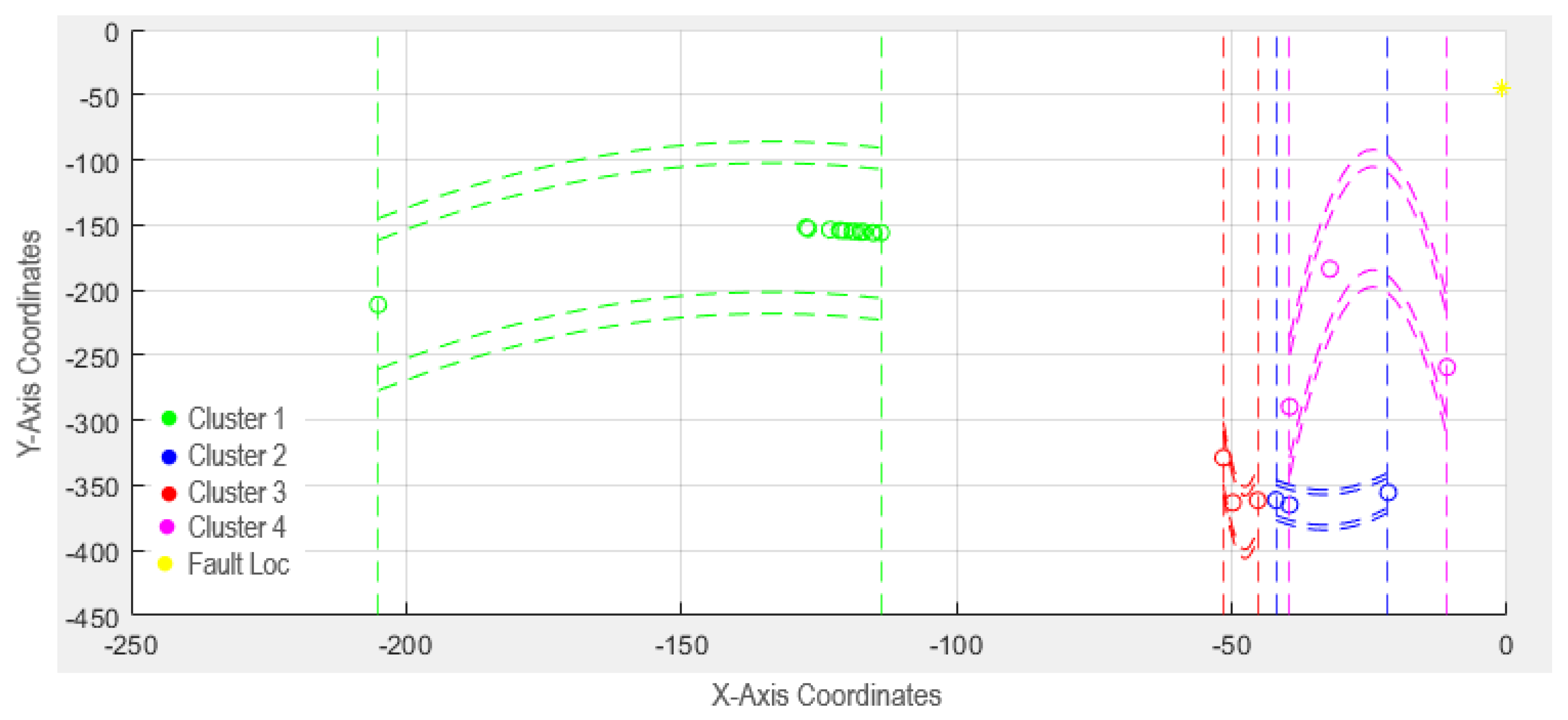
As stated in previous sections, the eigenvalues of each powerline have a distinct drift pattern in the eigenvalue space. These patterns are determined by the components that make up the impedance of the line, combined with the apparent impedance of the load. When foreign agents are introduced during abnormal conditions, such as a resistive element during a HIF, the eigenvalues of the line will drift away from their normal zones of operation. During a fault the eigenvalues of the line drift towards a point in the Eigenvalue Space determined by the characteristics of the fault. The higher the magnitude of the fault, the closer the eigenvalues move to this point in the Eigenvalue Space. For low impedance faults, this drift is quite dramatic, this is analogous to the changes in current magnitude seen during a bolted fault. Although not as dramatic as the changes seen during a bolted fault, the disturbances seen during a HIF are enough to produce a distinguishable deviation from the normal zones. This sensitivity to disturbances allows this solution to identify HIFs with a resistance of over 1 k Ω . 
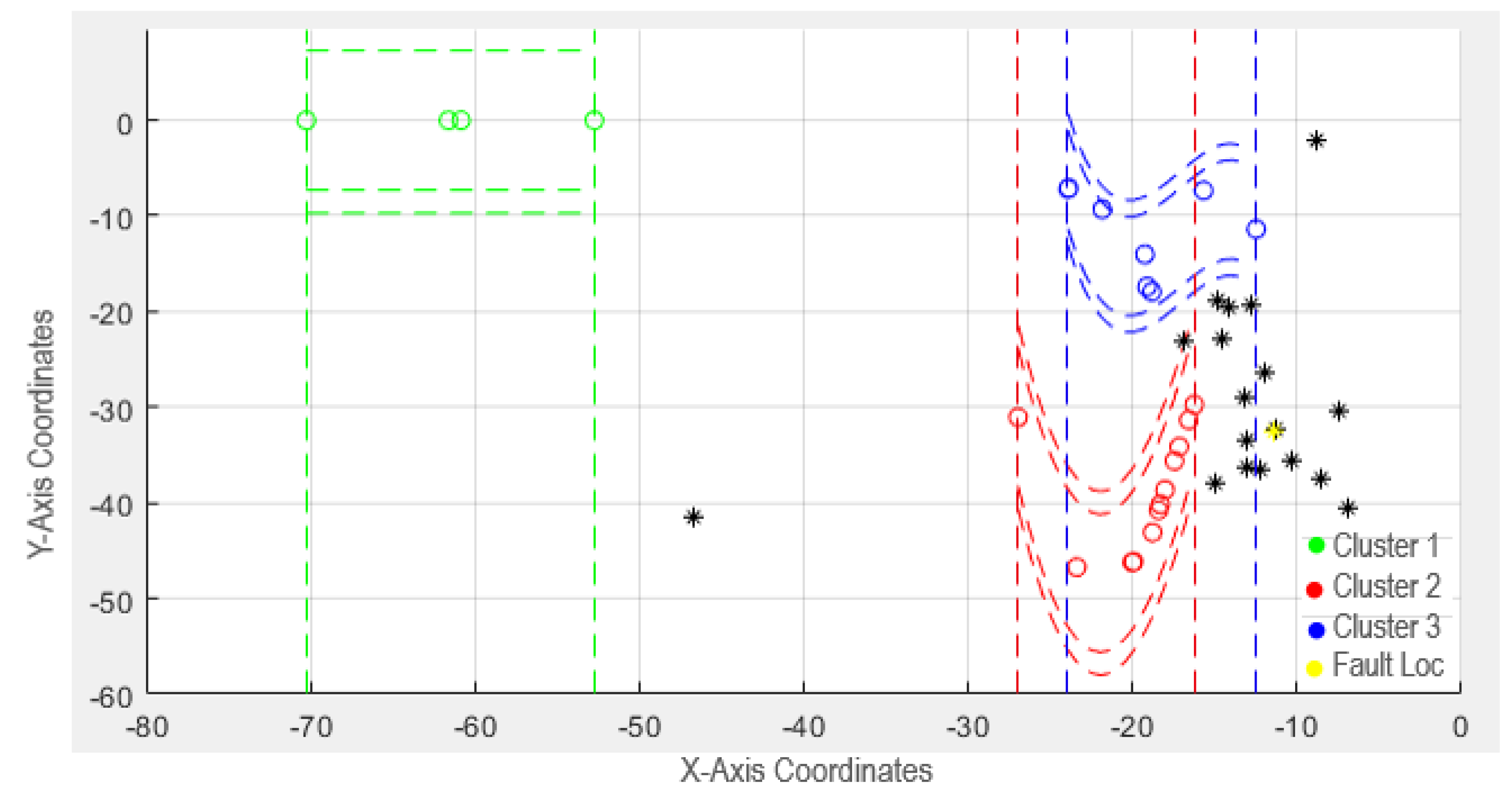
Figure 9 illustrates a case of eigenvalue drift during a fault with a resistance of 10 Ω , while Figure 10 shows the drift of eigenvalues in response to a fault with a resistance of 100 Ω .

3.4. Robustness to Noise

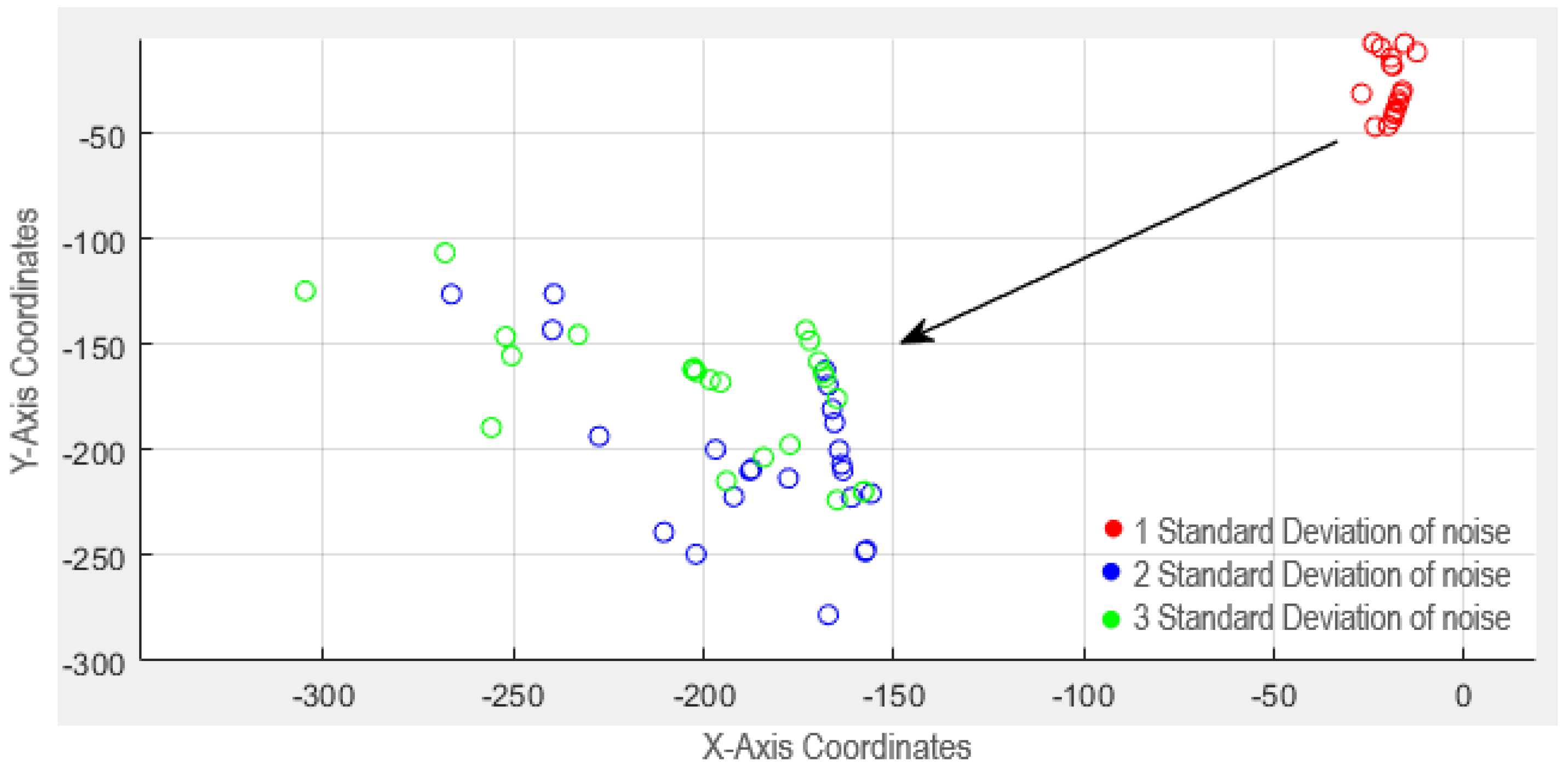
High sensitivity can be a double-edged sword as increased dependability can lead to false positives. The performance of the solution presented in this work was studied in the presence of noise. Noise injections do not change the general pattern followed by the eigenvalues, the overall pattern in simply shifted. Figure 11 illustrates this behavior.
In extreme cases where the magnitude of the noise can be classified as a gross error in measurement, the eigenvalues travel far beyond their normal zones, somewhat similar to the behavior seen during high magnitude faults. A scheme for the identification of gross errors in measurements can be developed from this solution: when the Subspace Estimator sees a dramatic Eigenvalue drift, the estimator could verify the status of the relay(s) protecting the line. If over-current elements in the relay have not been picked up, this would indicate an erroneous reading. This could improve the robustness of WAMS based State Estimation solutions.
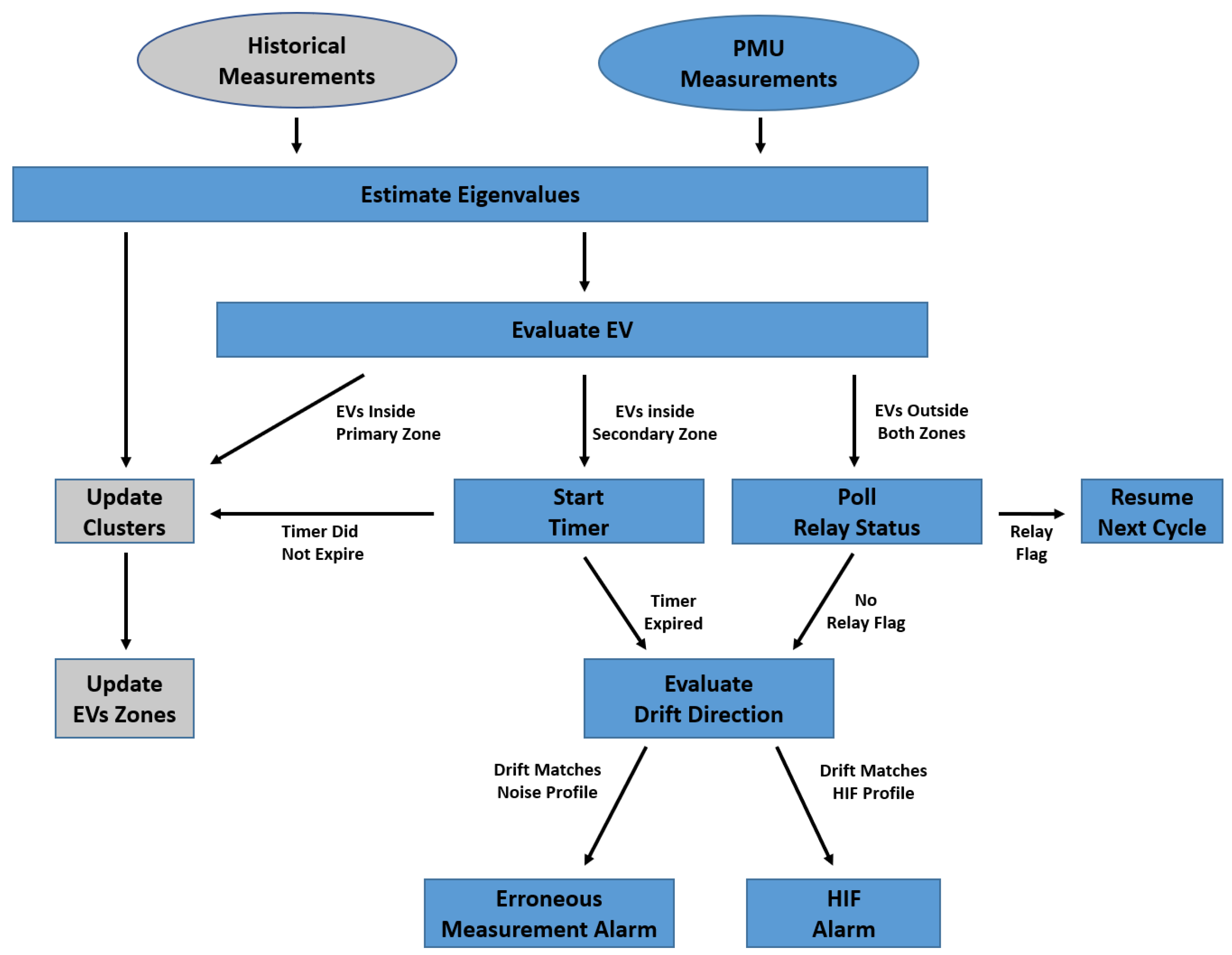
Eigenvalue space could also be integrated into relaying schemes to enhance the security of the scheme. Similar to a permissive scheme, a relay could poll the status of the estimator before sending a trip or a block command. Figure 12 illustrates the algorithm of the model introduced in this work.
A case study and the associated findings are presented in the next section.

4. Case Study

The I E E E 5-Bus system modeled in Matlab [30] is used to evaluate the performance of the framework presented in this work. Table 1 presents system data. Two scenarios were examined: First a single phase to ground fault is simulated on C-Phase of the line between Bus-4 and Bus-5. The results are presented in Fault Scenario I. Then, a single phase to ground fault is simulated on A-Phase of the line between Bus-1 and Bus-2. These results are presented in Fault Scenario II. Each scenario is set up as follows:
  • All Loads follow the trend shown in Figure 7.
  • The system is in steady state per the powerflow results shown in Table 2.
  • Each scenario consists of three fault iterations with fault resistances of 10 Ω , 100 Ω , and 1000 Ω .
  • During each iteration, the line is faulted twenty four (24) times to evaluate all the cluster zones and to account for dynamic loading conditions.
  • Clusters are built using historical loading data.
  • One standard deviation of Gaussian white noise is added to all the current measurements.

4.1. Fault Scenario I

Baseline eigenvalues are estimated as seen in Figure 13:
Clusters are generated using k-means clustering and the EDC, as seen in Figure 14:
The solution successfully detects a C-Phase to ground fault with a fault resistance of 10 Ω , as illustrated in Figure 15:
Statistics for this case study are presented in Table 3:
The solution successfully detects a C-phase to ground fault with a fault resistance of 100 Ω , as illustrated in Figure 16:
Statistics for this case study are presented in Table 4:
The solution successfully detects a C-phase to ground fault with a fault resistance of 1000 Ω , as illustrated in Figure 17:
Statistics for this case study are presented in Table 5:

4.2. Fault Scenario II

Baseline eigenvalues are estimated as seen in Figure 18:
Clusters are generated using k-means clustering and the EDC, as seen in Figure 19:
The solution successfully detects a C-phase to ground fault with a fault resistance of 10 Ω , as seen in Figure 20:
Statistics of this case study are presented in Table 6:
The solution successfully detects a C-phase to ground fault with a fault resistance of 100 Ω , as illustrated in Figure 21:
Statistics of this case study are presented in Table 7:
The solution successfully detects an C-phase to ground fault with a fault resistance of 1000 Ω , as illustrated in Figure 22:
Statistics for this case study are presented in Table 8:
As expected, during faults of lower impedance the profile of the estimated system is dominated by the fault. This pushes the eigenvalues far away from their normal zones as they congregate around a single point determined by the fault. The mean and standard deviation values seen during the 10 Ω and 100 Ω faults are evidence of this, as the values are almost the same for both fault conditions, and far from the normal values. In this context, a fault with a resistance of 100 Ω is considered a HIF, this illustrates the robustness of this framework.
At 1000 Ω , the eigenvalue drift is no longer dominated by the fault, however, the increase in resistance experienced by the system moves the Eigenvalues to new locations in the Eigenvalue Space. This deviation is still large enough for this solution to observe the change and issue an alarm.

5. Conclusions

This work presented a model for the detection of high impedance faults. The framework leverages WAMS technology, protective relaying schemes, and state estimation algorithms to produce a solution that yields high detection rates, 100% in the scenarios studied as part of this work. Encouraging results combined a philosophy that emphasizes generality, making this framework a promising alternative to solve the HIF problem. The performance of this method was studied in simulations based on I E E E benchmark systems. The key outcome of this work is a solution that is highly effective at detecting HIFs, well beyond 100 Ω of fault resistance. This is done by observing the characteristics of the system during normal operation and measuring deviations from the normal, in contrast to other HIF solutions, which focus on the characteristics of the faults.
Factors such as line impedance, loading on the line, and available fault current impact how the eigenvalues behave during normal operating conditions. To a lesser extent, these factors also affect how eigenvalues drift during fault conditions. Drift during fault conditions is mainly driven by the characteristics of the fault. The size of the system (the number of buses, lines, and sources) also has direct influence on the signature (eigenvalue drift pattern) of the lines. Changing the size of the system is equivalent to changing the overall impedance of the system. One of the strengths of the method presented in the paper is that it adapts to changing conditions and to virtually any topology. The only requirement is that the system be allowed to establish a baseline of acceptable values, and then the algorithm will look for deviations.
Presently, the main limitation of this framework seems to be distinguishing HIFs (over 500 Ω in fault resistance) from large injections of measurement noise, however, statistical tools and machine learning could hold the key to overcoming this challenge. Another limitation is the lack of a fault location module. Future work will focus on addressing those two limitations in addition to expanding the framework to include detection of faults of multiple impedance profiles and faults of a dynamic and transient nature.

Author Contributions

Conceptualization, G.P.; methodology, G.P.; software, G.P.; validation, G.P.; formal analysis, G.P.; investigation, G.P.; resources, G.P.; data curation, G.P.; writing—original draft preparation, G.P.; writing—review and editing, A.S.B.; visualization, G.P. and A.S.B.; supervision, A.S.B.; project administration, A.S.B.; funding acquisition, A.S.B. All authors have read and agreed to the published version of the manuscript.

Funding

This research was funded by NSF ECCS Award # 1809739.

Institutional Review Board Statement

Not applicable.

Informed Consent Statement

Not applicable.

Data Availability Statement

http://www.ercot.com/gridinfo/load (accessed on 10 October 2021).

Conflicts of Interest

The authors declare no conflict of interest.

References

  1. Rodriguez Paz, M.; Ferraz, R.; Bretas, A.; Leborgne, R. System unbalance and fault impedance effect on faulted distribution networks. Comput. Math. Appl. 2010, 60, 1105–1114. [Google Scholar] [CrossRef] [Green Version]
  2. Tampa Bay Times. A live power line lay on the ground for hours, unnoticed until it killed someone. How does that happen? Tampa Bay Times, 20 July 2016. [Google Scholar]
  3. Herrera-Orozco, A.; Bretas, A.; Orozco-Henao, C.; Iurinic, L.; Mora-Florez, J. Incipient fault location formulation: A time-domain system model and parameter estimation approach. Int. J. Electr. Power Energy Syst. 2017, 90, 112–123. Available online: https://www.sciencedirect.com/science/article/pii/S0142061516314028 (accessed on 15 May 2021). [CrossRef]
  4. Bretas, A.; Herrera-Orozco, A.; Orozco-Henao, C.; Iurinic, L.; Mora-Flórez, J. Incipient fault location method for distribution networks with underground shielded cables: A system identification approach. Int. Trans. Electr. Energy Syst. 2017, 27, e2465. [Google Scholar] [CrossRef]
  5. Orozco-Henao, C.; Bretas, A.; Marin-Quintero, J.; Herrera-Orozco, A.; Pulgarin-Rivera, J.; Velez, J. Adaptive Impedance-Based Fault Location Algorithm for Active Distribution Networks. Appl. Sci. 2018, 8, 1563. [Google Scholar] [CrossRef] [Green Version]
  6. Zou, T.; Aljohani, N.; Nagaraj, K.; Zou, S.; Ruben, C.; Bretas, A.; Zare, A.; McNair, J. A Network Parameter Database False Data Injection Correction Physics-Based Model: A Machine Learning Synthetic Measurement-Based Approach. Appl. Sci. 2021, 11, 8074. [Google Scholar] [CrossRef]
  7. Aljohani, N.; Bretas, A. A Bi-Level Model for Detecting and Correcting Parameter Cyber-Attacks in Power System State Estimation. Appl. Sci. 2021, 11, 6540. [Google Scholar] [CrossRef]
  8. Ramos, M.J.S.; Bretas, A.S.; Bernardon, D.P.; Pfitscher, L.L. Distribution networks HIF location: A frequency domain system model and WLS parameter estimation approach. Electr. Power Syst. Res. 2017, 146, 170–176. [Google Scholar] [CrossRef]
  9. Orozco-Henao, C.; Bretas, A.; Chouhy-Leborgne, R.; Herrera-Orozco, A.; Marín-Quintero, J. Active distribution network fault location methodology: A minimum fault reactance and Fibonacci search approach. Int. J. Electr. Power Energy Syst. 2017, 84, 232–241. [Google Scholar] [CrossRef]
  10. Bretas, A.; Bretas, N.; London, J.; Carvalho, B. Cyber-Physical Power Systems State Estimation; Elsevier: Amsterdam, The Netherlands, 2021. [Google Scholar]
  11. Bretas, N.; Bretas, A.; Martins, A. Convergence Property of the Measurement Gross Error Correction in Power System State Estimation, Using Geometrical Background. IEEE Trans. Power Syst. 2013, 28, 3729–3736. [Google Scholar] [CrossRef]
  12. Iurinic, L.; Herrera-Orozco, A.; Bretas, A.S. Distribution Systems High-Impedance Fault Location: A Parameter Estimation Approach. IEEE Trans. Power Deliv. 2016, 31, 1806–1814. [Google Scholar] [CrossRef]
  13. Ferraz, R.; Iurinic, L.; Filomena, A.; Gazzana, D.; Bretas, A. Arc fault location: A nonlinear time varying fault model and frequency domain parameter estimation approach. Int. J. Electr. Power Energy Syst. 2016, 80, 347–355. [Google Scholar] [CrossRef]
  14. Nam, S.R.; Park, J.K.; Kang, Y.C.; Kim, T.H. A Modeling Method of a High Impedance Fault in a Distribution System Using Two Series Time-Varying Resistances in EMTP. In Proceedings of the IEEE Power Engineering Society Summer Meeting, Vancouver, BC, Canada, 15–19 July 2001. [Google Scholar] [CrossRef]
  15. Bretas, N.; Bretas, A. The Extension of the Gauss Approach for the Solution of an Overdetermined Set of Algebraic Non Linear Equations. IEEE Trans. Circuits Syst. II Express Briefs 2018, 65, 1269–1273. [Google Scholar] [CrossRef]
  16. Bretas, N.G.; Bretas, A.S. A two steps procedure in state estimation gross error detection, identification, and correction. Int. J. Electr. Power Energy Syst. 2015, 73, 484–490. [Google Scholar] [CrossRef]
  17. Farias, P.E.; de Morais, A.P.; Rossini, J.P.; Cardoso, G. Non-linear high impedance fault distance estimation in power distribution systems: A continually online-trained neural network approach. Electr. Power Syst. Res. 2018, 157, 20–28. [Google Scholar] [CrossRef]
  18. Ramos, M.J.S.; Bretas, A.S.; Bernardon, D.P.; Pfitscher, L.L. Physics-based analytical model for high impedance fault location in distribution networks. Electr. Power Syst. Res. 2020, 188, 106577. [Google Scholar] [CrossRef]
  19. Nunes, J.U.N.; Bretas, A.S.; Bretas, N.G.; Herrera-Orozco, A.R.; Iurinic, L.U. Distribution systems high impedance fault location: A spectral domain model considering parametric error processing. Electr. Power Syst. Res. 2019, 109, 227–241. [Google Scholar] [CrossRef]
  20. Ghalei, M.; Zanjani, M.; Kargar, H.K.; Zanjani, M.G.M. High impedance fault detection of distribution network by phasor measurement units. In Proceedings of the 17th Conference on Electrical Power Distribution, Tehran, Iran, 1 May 2012. [Google Scholar] [CrossRef]
  21. Hossain, S.; Zhu, H.; Overbye, T. Distribution high impedance fault location using localized voltage magnitude measurements. In Proceedings of the 2014 North American Power Symposium (NAPS), Pullman, WA, USA, 7–9 September 2014. [Google Scholar] [CrossRef]
  22. Patynowski, D.; Cardenas, J.; Menendez, D.; Zhang, Z.; Roca, J.M.; Germain, J.G.; Huete, A.Y.; Canales, M.; Martinez, A.; Rosendo, J.A.; et al. Fault Locator approach for high-impedance grounded or ungrounded distribution systems using synchrophasors. In Proceedings of the 68th Annual Conference of Protective Relay Engineers, College Station, TX, USA, 30 March–2 April 2015. [Google Scholar] [CrossRef]
  23. RGKM Aarts. System identification and parameter estimation. In Lecture Notes; University of Twente: Enschede, The Netherlands, 2012. [Google Scholar]
  24. Trevizan, R.D.; Ruben, C.; Rossoni, A.; Dhulipala, S.C.; Bretas, S.A.; Bretas, N.G. µPMU-Based Temporal Decoupling of Parameter and Measurement Gross Error Processing in DSSE. Electricity 2021, 2, 25. [Google Scholar] [CrossRef]
  25. Bretas, A.; Bretas, N.; Massignan, J.; London Junior, J. Hybrid Physics-Based Adaptive Kalman Filter State Estimation Framework. Energies 2021, 14, 6787. [Google Scholar] [CrossRef]
  26. Horowitz, S.H.; Phadke, A.G. Power System Relaying, 4th ed.; Wiley: London, UK, 2014. [Google Scholar]
  27. MathWorks Cluster Analysis. 2021. Available online: https://www.mathworks.com/discovery/cluster-analysis.html (accessed on 30 July 2021).
  28. Singh, U.; Zamani, V.; Baran, M.E. Online load estimation for distribution automation using AMI data. In Proceedings of the 2016 IEEE Power and Energy Society General Meeting (PESGM), Boston, MA, USA, 17–21 July 2016. [Google Scholar] [CrossRef]
  29. ERCOT Grid Info: Load. Loading Data. 2021. Available online: http://www.ercot.com/gridinfo/load (accessed on 10 October 2021).
  30. Tan, R. IEEE 5-Bus System Model. Simulink Model. 2018. Available online: https://www.mathworks.com/matlabcentral/fileexchange/66555-ieee-5-bus-system-model (accessed on 3 October 2021).
Figure 1. Mho Relay Characteristic [26].
Applsci 11 12148 g001
Figure 2. Out of Step Relay characteristics [26].
Applsci 11 12148 g002
Figure 3. Diagram of the proposed configuration.
Applsci 11 12148 g003
Figure 4. RLC circuit schematic.
Applsci 11 12148 g004
Figure 5. Estimated eigenvalues in eigenvalue space.
Applsci 11 12148 g005
Figure 6. Houston load 24-h profile in PU [29].
Applsci 11 12148 g006
Figure 7. Low EDC cluster.
Applsci 11 12148 g007
Figure 8. High EDC cluster.
Applsci 11 12148 g008
Figure 9. Eigenvalue drift during a fault with a resistance of 10 Ω .
Applsci 11 12148 g009
Figure 10. Eigenvalue drift during a fault with a resistance of 100 Ω .
Applsci 11 12148 g010
Figure 11. Eigenvalue estimation in eigenvalue space with noise.
Applsci 11 12148 g011
Figure 12. Flowchart illustrating the eigenvalue space analysis model.
Applsci 11 12148 g012
Figure 13. Baseline eigenvalues.
Applsci 11 12148 g013
Figure 14. Clusters.
Applsci 11 12148 g014
Figure 15. 10 Ω fault identified.
Applsci 11 12148 g015
Figure 16. 100 Ω fault identified.
Applsci 11 12148 g016
Figure 17. 1000 Ω fault identified.
Applsci 11 12148 g017
Figure 18. Baseline eigenvalues.
Applsci 11 12148 g018
Figure 19. Clusters.
Applsci 11 12148 g019
Figure 20. 10 Ω fault identified.
Applsci 11 12148 g020
Figure 21. 100 Ω fault identified.
Applsci 11 12148 g021
Figure 22. 1000 Ω fault identified.
Applsci 11 12148 g022
Table 1. Impedance parameters of the 5-Bus system.
LineLine ImpedanceLine Charging
R (PU)X (PU)Y/2 (PU)
1–20.020.060.0 + j0.030
1–30.080.240.0 + j0.025
2–30.060.250.0 + j0.020
2–40.060.180.0 + j0.020
2–50.040.120.0 + j0.015
3–40.010.030.0 + j0.010
4–50.080.240.0 + j0.025
Table 2. Power flow results of the 5-Bus system.
BusGenerationDemandBus Voltage
MWMVARMWMVARVoltage (PU)Angle
1130−7.4001.060
2403020101.047−2.806
30045151.024−4.997
4004051.023−5.329
50060101.017−6.1503
Table 3. 10 Ω fault statistics.
Euclidean Distance StatisticsNormal ConditionsFault Conditions
Mean27.71250.3400
Standard Deviation18.93140.2334
Table 4. 100 Ω fault statistics.
Euclidean Distance StatisticsNormal ConditionsFault Conditions
Mean27.71251.3481
Standard Deviation18.93140.8519
Table 5. 1000 Ω fault statistics.
Euclidean Distance StatisticsNormal ConditionsFault Conditions
Mean27.7125171.1992
Standard Deviation18.9314228.4471
Table 6. 10 Ω fault statistics.
Euclidean Distance StatisticsNormal ConditionsFault Conditions
Mean109.43660.0213
Standard Deviation90.78640.0151
Table 7. 100 Ω fault statistics.
Euclidean Distance StatisticsNormal ConditionsFault Conditions
Mean109.43660.0215
Standard Deviation90.78640.0145
Table 8. 1000 Ω fault statistics.
Euclidean Distance StatisticsNormal ConditionsFault Conditions
Mean109.4366169.0397
Standard Deviation90.7864152.1032
Publisher’s Note: MDPI stays neutral with regard to jurisdictional claims in published maps and institutional affiliations.

