Article

Improving Multi-Label Learning by Correlation Embedding

1
School of Computer Science and Technology, Anhui University of Technology, Maanshan 243032, China
2
Key Laboratory of Data Science and Intelligence Application, Minnan Normal University, Zhangzhou 363000, China
3
Institute of Artificial Intelligence, Hefei Comprehensive National Science Center, Hefei 230088, China
*
Author to whom correspondence should be addressed.
Appl. Sci. 2021, 11(24), 12145; https://doi.org/10.3390/app112412145
Submission received: 18 November 2021 / Revised: 13 December 2021 / Accepted: 16 December 2021 / Published: 20 December 2021
(This article belongs to the Topic Machine and Deep Learning)

Abstract

:
In multi-label learning, each object is represented by a single instance and is associated with more than one class labels, where the labels might be correlated with each other. As we all know, exploiting label correlations can definitely improve the performance of a multi-label classification model. Existing methods mainly model label correlations in an indirect way, i.e., adding extra constraints on the coefficients or outputs of a model based on a pre-learned label correlation graph. Meanwhile, the high dimension of the feature space also poses great challenges to multi-label learning, such as high time and memory costs. To solve the above mentioned issues, in this paper, we propose a new approach for Multi-Label Learning by Correlation Embedding, namely MLLCE, where the feature space dimension reduction and the multi-label classification are integrated into a unified framework. Specifically, we project the original high-dimensional feature space to a low-dimensional latent space by a mapping matrix. To model label correlation, we learn an embedding matrix from the pre-defined label correlation graph by graph embedding. Then, we construct a multi-label classifier from the low-dimensional latent feature space to the label space, where the embedding matrix is utilized as the model coefficients. Finally, we extend the proposed method MLLCE to the nonlinear version, i.e., NL-MLLCE. The comparison experiment with the state-of-the-art approaches shows that the proposed method MLLCE has a competitive performance in multi-label learning.

1. Introduction

In multi-label learning, each object is represented by a single instance and is associated with multiple class label [1,2,3]. The main task of learning is to build an effective classifier based on the training data and predict the most relevant set of labels for each unseen instance. Nowadays, multi-label learning has been applied in various fields [1,4], such as music emotion classification [5], video classification [6], Internet [7], text classification [8,9], and information retrieval [10].
In recent years, multi-label learning has attracted extensive attentions from researchers. Existing research has demonstrated that exploiting label correlation can provide important information for the prediction of new instances and significantly boost classification performance. For example, if a piece of news is related to the theme of “Olympics”, it is more likely to belong to the theme of “sports” and “culture”, vice versa, “war” is unlikely. When an image was annotated with “reef”, the probability of being annotated with “waves” will be very high, and the probability of being annotated with “desert” will be very low.
Through the investigation and research of previous work on multi-label learning, a lot of methods [11,12,13,14,15] have been proposed by exploiting label correlations. For example, in CLR [14], an extra calibration label is introduced and utilized to separate the relevant and irrelevant labels for each instance. JFSC [15] learns the label-specific and shared features based on pairwise label correlation. In DLCL [12], a novel multi-label learning method is proposed, which can find the latent class labels in the training data. DLCL exploits the correlation between known and latent class labels to enhance the performance of the classifier. The Maximal Correlation Embedding Network (MCEN) uses the label similarity by embedding the maximum correlations in the label space to solve the problem of missing labels [16]. MLC-EBMD [17] introduces a multi-label classification framework based on Boolean matrix decomposition to improve the ability to predict labels in high-dimensional label space, and it also performs dimension reduction in the feature space.
The aforementioned methods definitely enhance the prediction accuracy of the multi-label algorithm by resolving and using the correlation of label. These methods on modeling label correlation mainly use either popular regular constraints, which means that any two labels with a strong relationship are assigned to similar model coefficients, or label ranking. It is noted that these methods mainly model label correlations in an indirect way, i.e., adding extra constraints on the coefficients or outputs of a multi-label classification model based on a pre-learned label correlation graph. However, in such an indirect way on modeling label correlation, the inherent correlations between different labels will not be well kept. It would be better if a direct way could be proposed. Moreover, in the environment of big data, it is convenient to collect a massive amount of data. However, the curse of dimension has brought great obstacles to multi-label learning.Therefore, it is wise to construct learning models in the low-dimensional feature and label space [18,19,20].
To solve the above mentioned issues, in this paper, we propose a new approach for Multi-Label Learning by Correlation Embedding, namely MLLCE, where the feature space dimension reduction and the multi-label classification are integrated into a unified framework. First, we project the original high-dimensional feature space to a low-dimensional latent space by a mapping matrix. To model label correlation, we learn an embedding matrix from the pre-defined label correlation graph by graph embedding. Then, we use the embedding matrix as the model coefficients to construct a multi-label classifier from the low-dimensional latent feature space to the label space. In this way, the inherent correlations between different labels will be directly kept in the model coefficients. Finally, we extend the proposed method MLLCE to the nonlinear version, i.e., NL-MLLCE. The comparison experiment with the state-of-the-art approaches shows that the proposed method MLLCE has a competitive performance in multi-label learning.
The rest of this paper is organized as follows. Section 2 reviews the previous methods of using label correlation for multi-label learning. Section 3 introduces the proposed method MLLCE in detail. Comparative experiment results and analyses are presented in Section 4. Finally, we conclude this paper in Section 5.

2. Related Works

In multi-label learning, mining the correlation among labels can provide important information, make the prediction results more accurate, and boost the performance of the model. According to the ways on modeling label correlations, existing multi-label learning algorithm can be divided into three categories, i.e., first-order, second-order, and high-order algorithms. The first-order methods [21,22] deal with multi-label classification problems without modeling the label correlations. BR [21] is a typical first-order algorithm whose basic idea is to transform a multi-label learning problem into multiple independent binary classification problems. The second-order methods exploit the pairwise relationship between labels [23,24,25]. For the high-order methods, the relationship between all class labels or a subset is modeled, such as [26,27,28]. For example, the classifier chain (CC) [29] is a chain algorithm that uses a vector of class labels as additional instance attributes to model high-order label correlation. The Probabilistic Classifier Chain (PCC) [30] is a probabilistic version of CC. LELC [31] combines label embedding and label correlation to solve multi-label text classification problems. HIDDEN [32] learns the hierarchical multi-label classification based on the joint learning of document classifier and label embedding. ELM-LMF [33] generates the latent label matrix and k-label dependency matrix based on the label matrix decomposition. CLP-RNN [34] is a multi-label classification method that allows the selection of dynamic and context-dependent label ordering based on label embedding. The MLL-FLSDR [20] algorithm is a multi-label learning method for solving the problem with many labels and features based on the label embedding, which reduces the dimension in both feature space and label space.
The second-order methods deal with the multi-label learning problem by exploring the pairwise relationship between the labels that can be divided into two types. First, the second-order methods incorporate the classification criteria ranking loss into the objective function of multi-label learning, such as Rank-SVM [23], MIMLfast [24], and LSEP [25]. Second, the second-order methods constrain the label correlations to the model coefficients or outputs, such as [11,35,36,37,38]. LLSF [35] used the correlation between the labels to learn specific label features for multi-label learning. LSF-CI [36] is a multi-label feature multi-label learning method which considered the relevant information of the label space and the feature space simultaneously. There are also some algorithms that tend to investigate global and local label correlations. ML-LOC [11] exploits local pairwise label correlation for multi-label learning. LF-LPLC [37] learns specific label features and exploits local pairwise label correlation for multi-label learning. GRRO [38] is a multi-label feature selection method that exploits the global pairwise label correlation to facilitate the selection of features. These algorithms only utilize positive label correlation between labels, while some of the label are negatively correlated or mutually exclusive with each other. To solve this problem, several algorithms have been proposed to model the negative correlation between labels. For example, the LPLC [39] is a simple and effective Bayesian model to investigate the positive correlation and negative correlation between the labels, and it finds the positive and negative relevance class labels for each label. Nan et al. [40] exploited the local positive and negative correlation between labels through kNN method. Most of these multi-label learning algorithms model label correlation with external conditions, and may not be able to maintain the correlation structure of labels well.
Dimension reduction is a fundamental pre-processing procedure for high-dimensional data, and many methods have been proposed for multi-label learning, such as MLDA [41], SSMLDA [42], and MLLS [43]. Through the overview of dimension reduction [44], dimension reduction can basically be divided into three categories, i.e, dimension reduction of the feature space, dimension reduction of the label space, and dimension reduction of the label and feature spaces simultaneously. PCA [45] is a method of dimension reduction in feature space based on label-independence. DCR [46] is a new multi-label feature selection method by combining feature relevance and label relevance. In [47], the authors propose a dimension reduction method DSE to learn the sparse weight matrix by projecting the original sample into a low-dimensional subspace. MDDM [48] is a multi-label dimension reduction approach based on maximizing the dependency between feature descriptions and relevant class labels. CLEMS [49] performs the dimension reduction of the label space through embedded instances. In addition, some methods are proposed to reduce dimension of the label space, such as [50,51]. GIMC [52] learns a nonlinear mapping of the features by reducing the instance features and labels.
In the environment of big data, the feature space of data sets becomes larger and larger, adopting dimension reduction, which can help to get rid of redundant features and obtain a more compact feature space, and further improve the performance of a model. To solve the above mentioned issues, in this paper, we propose a new approach for Multi-Label Learning by Correlation Embedding, namely MLLCE, where the feature space dimension reduction and the multi-label classification are integrated into a unified framework. We learn an embedding matrix from the pre-defined label correlation graph by graph embedding and utilize the embedding matrix as the model coefficients.

3. The Proposed Method

In multi-label learning, X = [ x 1 , x 2 , , x n ] T R n × d is the feature matrix and Y { 0 , 1 } n × q is the label matrix, where n is the number of instances, d is the dimension and q is the number of class labels. The i-th example is denoted by a vector with d attribute values x i = [ x i 1 , x i 2 , , x i d ] , and y i = [ y i 1 , y i 2 , , y i q ] is a set of possible labels for x i , where y i j = 1 indicates the i-th instance belonging to the j-th label, otherwise, y i j = 0 .
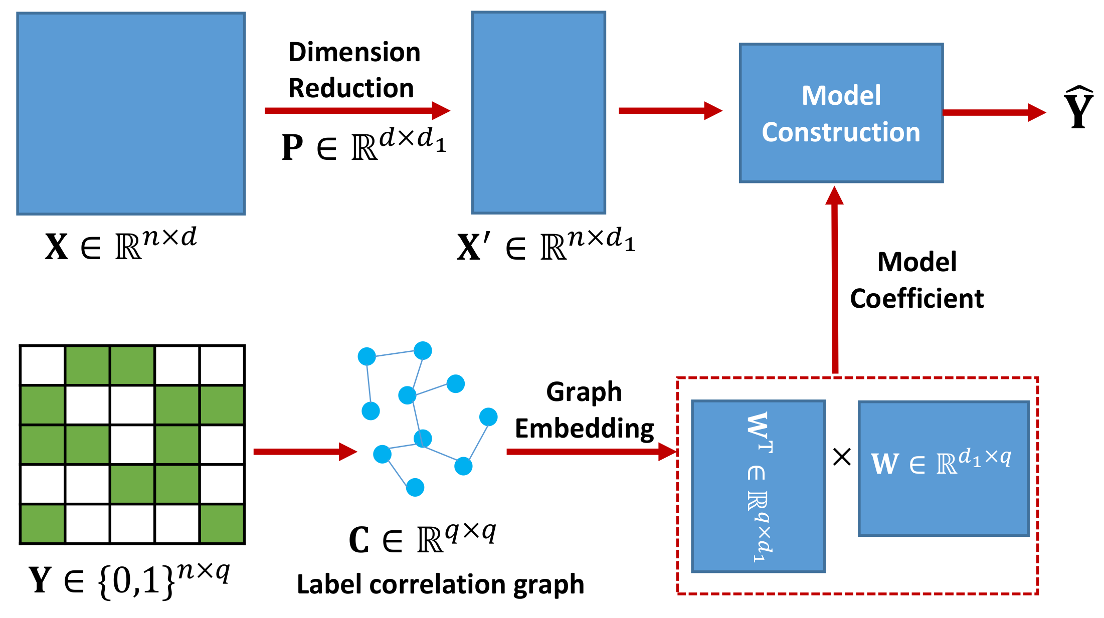
In this paper, we integrate the feature space dimension reduction and the multi-label classification into a unified framework. The learning framework of our proposed method MLLCE is shown in Figure 1. First, we project the original high-dimensional feature space to a low-dimensional latent space by a mapping matrix. To model label correlation, we learn an embedding matrix from the pre-defined label correlation graph by graph embedding. Then, we use the embedding matrix as the model coefficients to construct a multi-label classifier from the low-dimensional latent feature space to the label space. In this way, the inherent correlations between different labels will be directly kept in the model coefficients. Finally, we extend the proposed method MLLCE to the nonlinear version, i.e., NL-MLLCE.

3.1. Label Correlation Embedding

Exploiting the label correlation can improve the generalization ability of a model and significantly improve the accuracy of model prediction in multi-label learning [53,54]. In this paper, we model the label correlation under the second-order strategy.
First, we calculate the label correlation matrix C R q × q by cosine similarity based on the label matrix Y { 0 , 1 } n × q , where n represents the number of samples, and q indicates the number of labels. Each element C i j indicates the correlation between the i-th and j-th labels, and it is obtained by Equation (1).
C i j = h = 1 n Y h i Y h j / h = 1 n Y h i 2 h = 1 n Y h j 2
where Y h i represents the value of the element in the h-th row and i-th column of Y , and Y h j represents the value of the element in the h-th row and j-th column of Y .
Second, we decompose the label correlation matrix C into a low-dimensional space by graph embedding as follows
min W λ 1 4 | | C W T W F 2 .
For W , we can utilize it as the model coefficient to construct a multi-label classifier. In this paper, we first construct a linear model for multi-label classification as follows
min W 1 2 | | X W Y F 2 + λ 1 4 | | C W T W F 2 + λ 2 2 W 21 ,
where W = [ w 1 , w 2 , , w q ] R d × q , λ 1 and λ 2 are non-negative weight parameters. The 21 -norm regularization term is imposed on W to ensure the sparsity, which can select discriminative features. In addition, 21 norm has been confirmed to be robust to outliers and noise [55].
Previous studies mainly constrain the correlation between labels on the model coefficient matrix or the output by manifold regularization [35,36]. Different from previous studies, we directly model the pairwise label correlations by graph embedding, and the structure of label correlation will be well kept in W .

3.2. Dimension Reduction

During the past decades, multi-label classifiers are generally constructed from the feature space to the label space [56,57] directly. However, the high dimension of multi-label data in the feature space puts great pressure on time and memory costs. To address this issue, we explicitly introduce a feature dimension reduction stage that the data is projected from the original feature space to the low-dimensional feature space by mapping matrix.
We adopt the multiple linear regression model to build a linear classification model f ( X , P , W ) = X P W from the low-dimensional feature space to the label space, where P R d × d 1 is the feature mapping matrix, and W R d 1 × q is the model coefficient matrix. Consequently, the objective function can be rewritten as follows
min P , W 1 2 | | X P W Y F 2 + λ 1 4 | | C W T W F 2 + λ 2 2 W 21 .
For any matrix W R m × n , W F 2 = i = 1 m j = 1 n W i j 2 = tr ( W T W ) , The 21 of W is defined as W 21 = i = 1 m j = 1 n W i j 2 . Consequently, we can rewrite the third term W 21 by 2 tr ( W T D W ) , where D is a diagonal matrix with its diagonal element D i i = 1 2 W i : T W i : + ε and ε is a small positive constant. As a result, the objective function becomes
min P , W 1 2 | | X P W Y F 2 + λ 1 4 | | C W T W F 2 + 2 λ 2 tr ( W T D W ) .

3.3. Optimization

For problem (5), it is convex, and there are two parameters, i.e., W and P . We adopt the effective alternate optimization strategy. Specifically, in each iteration, we update one parameter and fix the other one. We use F ( ψ ) to represent the objective function in problem (5), where ψ = { P , W } indicates the set of the two parameters.

3.3.1. Update P

By fixing W , the problem (5) is simplified as
min P 1 2 | | X P W Y F 2 .
Then, we can obtain the gradient w.r.t P as
P F = X T XPW W T X T Y W T .
According the gradient descend algorithm, P can be updated by
P = P λ p P F ,
where λ p is step size of P in the gradient descent update rules. Choosing an appropriate step size is crucial to improve the convergence rate and reduce the total running time of MLLCE. According to the literature [58], we adopt the Armijo rule to automatically determine the step size λ p in each iteration.

3.3.2. Update W

With P fixed, the Equation (5) becomes:
min W 1 2 | | X P W Y F 2 + λ 1 4 | | C W T W F 2 + 2 λ 2 tr ( W T D W )
Therefore, we can obtain the gradient w.r.t W as
W F = P T X T XPW P T X T Y + λ 1 ( W W T W ) + 2 D W .
Consequently, W can be updated by
W = W λ w W F .
Similarly, the step size λ w is also determined by the Armijo rule [58]. According to the above optimization process, we give the pseudo code of the proposed method MLLCE in Algorithm 1.
Algorithm 1: Improving Multi-Label Learning by Correlation Embedding
Applsci 11 12145 i001

3.4. Non-Linear Extension of MLLCE

In addition, by considering nuclear techniques [59], a non-linear version of the MLLCE method can be derived by introducing the kernel trick. Specifically, we adopt a nonlinear feature mapping Φ ( · ) : R d R Ψ , which maps the original feature space to the higher-dimensional Reproducing Kernel Hilbert Space (RKHS). Accordingly, the feature mapping matrix is set to be P = Φ H , where Φ = [ Φ ( x 1 ) , Φ ( x 2 ) , , Φ ( x n ) ] R Ψ × n , H R n × d . The kernel matrix is usually given as K = Φ ( x ) T Φ ( x ) R n × n , Φ ( x ) T P = Φ ( x ) T Φ ( x ) H = K H .
Consequently, for the nonlinear version of MLLCE, the objective function of problem (5) can be rewritten as
min H , W 1 2 | | K H W Y F 2 + λ 1 4 | | C W T W F 2 + λ 2 W 21 .
Then, similar to the optimization of the linear version of MLLCE method, W and H are updated through an effective alternate optimization manner. The specific optimization process is based on Equations (7)–(11).

3.5. Complexity Analysis

For the proposed approach, data matrix X R n × d , projection matrix P R d × d 1 , W R d 1 × q , label matrix Y { 0 , 1 } n × q , D R d 1 × d 1 , label correlation matrix C R q × q , which n and q are the number of instance and label respectively, d and d 1 are the dimension of the original and the low-dimensional feature space.
In Algorithm 1, steps 5–7 are the most time-consuming parts. For steps 5 and 6, the update needs to be calculated by steps 2 and 3, in which the calculation mainly consists of some matrix multiplications. Therefore, the total time complexity is O ( t ( n d 2 + n d q + n d d 1 + n d 1 q + d 2 d 1 + d d 1 q + d d 1 2 + d 1 2 q ) ) , where t is the number of iterations. After the optimization, we only need to save P and W , it can lead to a memory cost of O ( d 1 q + d d 1 ) .

4. Experiment

4.1. Comparing Algorithms

In order to verify the performance of our proposed method, the paper selects five existing state-of-the-art multi-label classification approaches to compare with MLLCE, i.e., BR, JFSC, ML-LSS, MLL-FLSDR, and Glocal. The detailed information regarding the method of comparison and the linear and non-linear proposed in this paper are as follows:
(1)
BR [21]: The basic idea of BR is to decompose a multi-label learning problem into a set of independent binary classification sub-problems. In this paper, linear regression is adopted as the base learner for each binary classification sub-problem, where the regularization parameter is searched in { 0.1 , 1 , , 10 } .
(2)
JFSC [15]: JFSC is a feature selection and multi-label classification algorithm by exploiting label correlation. The search scope for parameters α , β and γ are { 4 5 , 4 4 4 5 } . Parameter η is searched in { 0.1 , 1 , , 10 } .
(3)
ML-LSS [60]: ML-LSS is proposed for multi-label learning by modeling local similarity. Parameter λ 1 , λ 2 are tuned in { 2 5 , 2 4 , , 2 6 } .
(4)
MLL-FLSDR [20]: A multi-label learning method based on label embedding that is used to solve the problem of many labels and features, where the parameter λ 1 is searched in { 10 2 , 10 3 , , 10 6 } , λ 2 , and λ 3 and λ 4 are searched in { 10 3 , 10 2 , , 10 1 } .
(5)
Glocal [61]: A multi-label learning approach that utilized the global and local label correlation. The parameter λ = 1 and the parameters λ 1 to λ 5 are tuned in { 10 5 , 10 4 10 1 } , k is searched in { 0.1 l , 0.2 l 0.6 l } , where l is the number of labels in each data set. g is searched in { 5 , 10 , 15 , 20 } .
(6)
MLLCE and NL-MLLCE:The two versions of our proposed method in this paper. Parameter λ 1 and λ 2 are tuned in { 10 6 , 10 4 , , 10 2 } . d 1 = 0.3 d is the feature dimension in the low feature space, where d is the dimension of the original feature space.

4.2. Data Sets

In this paper, a total of 15 multi-label benchmark data sets are used to verify the effectiveness of our method. Detailed information about these data sets are summarized in Table 1. For each data set S, | S | denotes the number of instances, d i m ( S ) denotes the number of features, and L ( S ) denotes the number of labels. In addition, L C a r d ( S ) is cardinality, which indicates the average number of labels belonging to instances, and r D e p ( S ) denotes the ratio of unconditionally dependent label pairs.

4.3. Evaluation Metrics

A great many evaluation metrics have been proposed to evaluate the performance of multi-label learning algorithms. In the paper, we choose six common evaluation metrics. Define a test data T = { ( x 1 , Y 1 ) , ( x 2 , Y 2 ) ( x 1 , Y n t ) } , where the ground truth labels set of the instance x i is represented as Y i { 0 , 1 } q , Y i Y , h ( x i ) { 0 , 1 } q is the set of predicted class labels for the i-th instance, f ( x i , y ) is the the confidence score that x i belongs to label y.
Hamming Loss evaluates the error between the predicted label of each instance obtained by the model and the true label of each instance.
Hamming Loss = 1 n t i = 1 n t 1 l | h ( x i ) Δ Y i |
where Δ indicates the symmetric difference between two sets.
One Error evaluates the proportion of instances whose top-ranked label is not in the ground truth label set.
One Error = 1 n t i = 1 n t [ arg max y Y f ( x i , y ) ] Y i
where · represents the indication function.
Ranking Loss indicates how many irrelevant labels are ranked higher than related labels.
Ranking Loss = 1 n t i = 1 n t 1 | Y i | | Y i ^ | | { ( y , y ) | f ( x i , y ) f ( x i , y ) , ( y , y ) Y i × Y i ¯ } |
Average Precision evaluates the proportion of the label that is ranked before the relevant label of the instance is still the related label.
Average Precision = 1 n t i = 1 n t 1 | Y i | y Y i | { y | r a n k f ( x i , y ) r a n k f ( x i , y ) , y Y i } | r a n k f ( x i , y )
Micro F1-Measure evaluates the prediction performance of the learned classifier on the label set.
MicroF 1 = 2 i = 1 n t | h ( x i ) Y i | i = 1 n t | Y i | + i = 1 n t | h ( x i ) |
Example-based F1 is the integrated version of precision and recall for each instance.
Example - based F 1 = 1 n t i = 1 n t 2 p i r i p i + r i
where p i and r i are the precision and recall for the i-th instance.
Macro AUC evaluates the probability that a positive instance is ranked before a negative instance, averaged over all labels.
AUC = 1 l i = 1 l | { ( x , x ) | f ( x , y j ) f ( x , y j ) , ( x , x ) Z j × Z j ¯ } | | Z j | | Z j ¯ |
where Z j = { x i | y j Y i , 1 i l } ( Z j ¯ = { x i | y j Y i , 1 i l } ) indicates that it does not belong to a set of test instances labeled y j .
For the AUC and AP evaluation metrics, the larger the value, the better the classification result. Hamming loss, One Error, Ranking Loss, and Coverage value are smaller, indicating better classification performance.

4.4. Experimental Results

For each data set, 80% is used for training and 20% is used for test set. The average value as well as standard deviation of each comparison algorithm in terms of each the evaluation metric are recorded in Table 2, Table 3, Table 4, Table 5, Table 6, Table 7 and Table 8 for 13 data sets. The best results in each row of the table will be emphasized in bold.
To further understand whether MLLCE makes a significant performance difference, we adopt the Wilcoxon signed-rank test [62]. For any pair of two comparing classifiers, the test can return three probabilities between them: the probability that the first classifier has a higher score than the second (left), the probability that differences are within the region of practical equivalence (rope), or that the second classifier has a higher score (right). The sum of the probabilities of left, right, and rope is 1. The larger the value of left or right, the better the performance of the first or second classifier is. A large value of rope indicates that there is no significant difference in the performance between the two classifiers. The results of Wilcoxon signed-rank test in terms of seven metrics are reported in Table 9, Table 10, Table 11 and Table 12.
Based on the experimental results, we can observe the following conclusions.
  • The linear and the nonlinear versions of the method MLLCE have comparable performance. In addition, the nonlinear MLLCE is better than the MLLCE method in terms of average precision, ranking loss, one error, and AUC, which indicates that the proposed nonlinear method can improve classification performance to some extent.
  • Compared to the the five comparison methods, MLLCE achieves competitive performance in terms of ranking loss, Micro F1, AUC, one error, average precision, Example-based F1 on the 15 data sets, and these results clearly show the effectiveness of MLLCE in multi-label learning.
  • In Hamming loss, the performance of all the comparing algorithms are not significantly different. However, according to Table 2, it is noted that MLLCE still achieves a relatively good performance.
  • MLLCE outperforms ML-LSS and Glocal on all evaluation metrics except hamming loss, Micro F1 and Example-based F1 Since ML-LSS adds sample similarity to the model, ML-LSS has better performance in Micro F1 and Example-based F1 metrics. These results verify the feasibility of our proposed method MLLCE through graph embedding to model label correlation.

4.5. Sensitivity Analysis

There are three parameters λ 1 , λ 2 and d 1 in our paper, where parameter λ 1 controls the loss of matrix embedding of label correlation C . The parameter λ 2 controls the sparsity of the model coefficient matrix W . Parameter d 1 indicates the reduced feature space dimension.
The search range of parameter λ 1 and λ 2 regarding the linear and nonlinear MLLCE methods proposed in the paper are both { 10 i | i = 3 : 2 } . The variation range value of low-dimensional feature dimension d 1 is { 15 % d , 19 % d 15 % d } , 
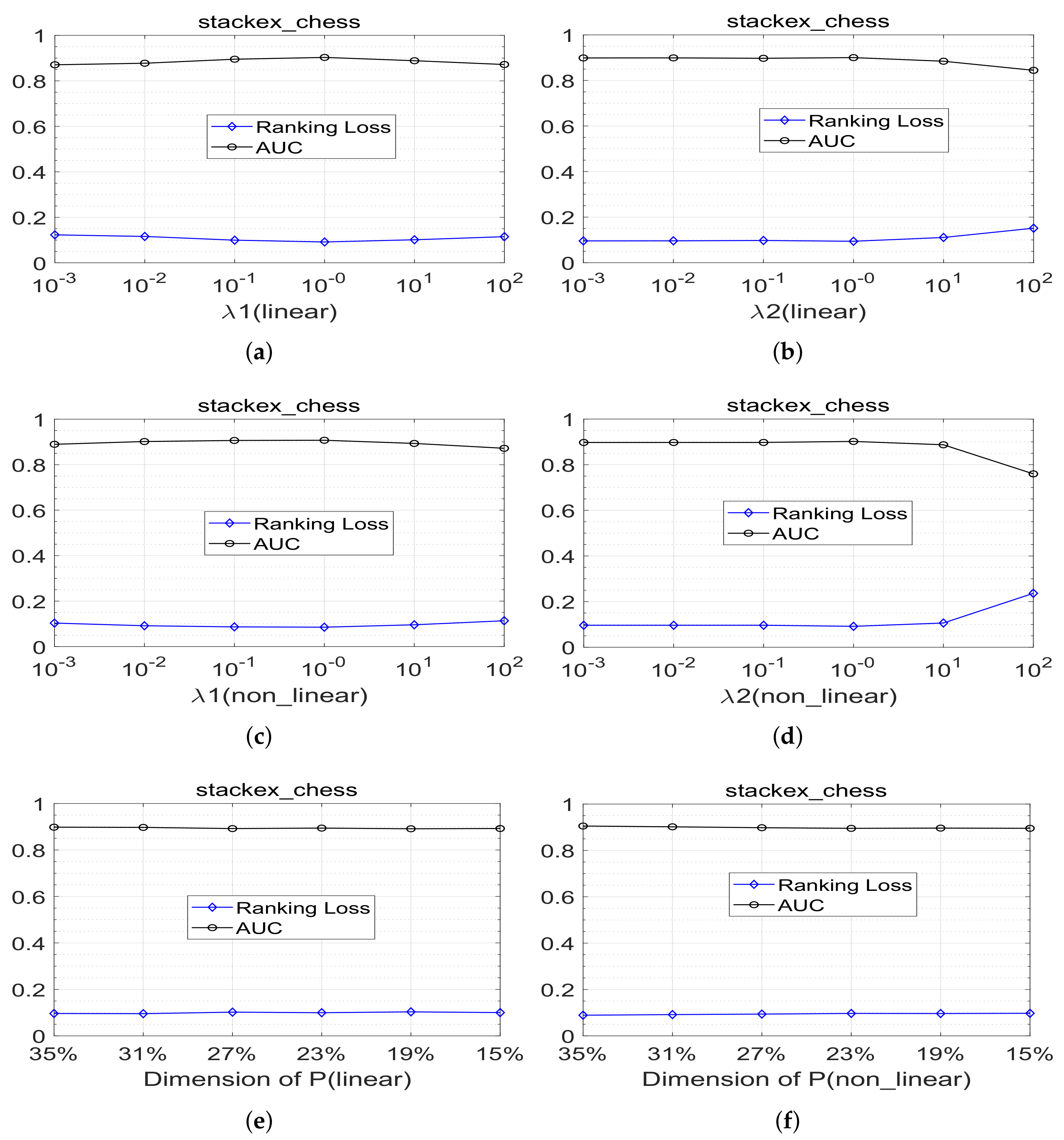
d is the dimension of the original feature space on each data set. We perform the experiment on stackex-chess data set by dividing the 80% training and 20% test part of data set five times randomly. Figure 2a–d shows the average experimental results of parameters λ 1 and λ 2 with different values in terms of the evaluation metric ranking loss and AUC. Figure 2e,f shows the average experimental results of MLLCE with different values of d 1 in terms of the evaluation metric ranking loss and AUC. We can note that the performance of MLLCE is not so sensitive to the value of d 1 .

4.6. Convergence

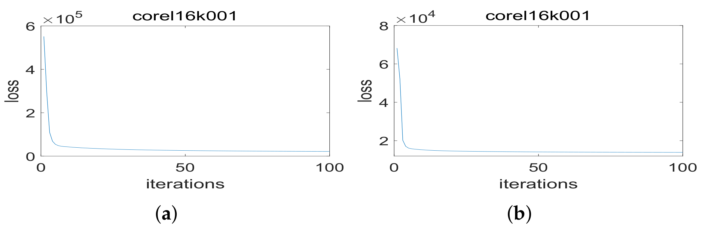
To illustrate the convergence of the proposed method, Figure 3 shows the change curve of the total loss of the objective function of the linear and nonlinear MLLCE as the number of iteration increases on data set corel16k001. In the experiment, we set that if the total loss of the objective function decreases less than 10 4 after an alternate iteration, the iterative optimization process will be terminated. As shown in Figure 3, the total loss value is rapidly reduced in the initial iteration and gradually converges with the iterative optimization process.

5. Conclusions

In this paper, we propose a new multi-label learning method by correlation embedding. First, we project the original high-dimensional feature space to a low-dimensional latent space by a mapping matrix. Then we learn an embedding matrix from the pre-defined label correlation graph by graph embedding, where the embedding matrix is utilized as the model coefficients. By learning such a classifier, the structure of the correlation matrix can be kept. In addition, the constraint of 21 norm regularization on the W can further reduce the size of the model. The experimental results show the effectiveness of our proposed linear and nonlinear MLLCE. Finally, the model of our proposed method is not complicated, and future work will focus on adding some constraints to improve this model.

Author Contributions

Investigation, J.H. and Q.X.; Methodology, J.H.; software, Q.X.; validation, X.Q. and Y.L.; writing-original draf, Q.X.; writing—review & editing, J.H., X.Q., Y.L. and X.Z. All authors have read and agreed to the published version of the manuscript.

Funding

This work was funded by NSFC: 61806005, The University Synergy Innovation Program of Anhui Province: GXXT-2020-012, The Key Laboratory of Data Science and Intelligence Application, Minnan Normal University (NO.D202003), and Natural Science Foundation of the Educational Commission of Anhui Province of China: KJ2018A0050. The APC was funded by Natural Science Foundation of the Educational Commission of Anhui Province of China: KJ2018A0050.

Institutional Review Board Statement

Not applicable.

Informed Consent Statement

Not applicable.

Data Availability Statement

The experimental datasets are available at http://www.uco.es/kdis/mllresources/.

Conflicts of Interest

The authors declare no conflict of interest.

References

  1. Zhang, M.-L.; Zhou, Z.-H. A Review on Multi-Label Learning Algorithms. IEEE Trans. Knowl. Data Eng. 2014, 26, 1819–1837. [Google Scholar] [CrossRef]
  2. Du, J.; Vong, C.-M. Robust Online Multilabel Learning Under Dynamic Changes in Data Distribution With Labels. IEEE Trans. Cybern. 2020, 50, 374–385. [Google Scholar] [CrossRef]
  3. Xu, M.; Li, Y.-F.; Zhou, Z.-H. Robust Multi-Label Learning with PRO Loss. IEEE Trans. Knowl. Data Eng. 2020, 32, 1610–1624. [Google Scholar] [CrossRef] [Green Version]
  4. Zhang, M.-L.; Li, Y.-K.; Liu, X.-Y.; Geng, X. Binary relevance for multi-label learning: An overview. Front. Comput. Sci. 2017, 12, 191–202. [Google Scholar] [CrossRef]
  5. Wu, B.; Zhong, E.; Horner, A.; Yang, Q. Music Emotion Recognition by Multi-label Multi-layer Multi-instance Multi-view Learning. In Proceedings of the MM 2014—2014 ACM Conference on Multimedia, Orlando, FL, USA, 3–7 November 2014; pp. 117–126. [Google Scholar] [CrossRef]
  6. Qi, G.-J.; Hua, X.-S.; Rui, Y.; Tang, J.; Mei, T.; Zhang, H.-J. Correlative multi-label video annotation. In Proceedings of the 15th International Conference on Multimedia—MULTIMEDIA ’07, Augsburg, Germany, 24–29 September 2007; ACM Press: New York, NY, USA, 2007; pp. 17–26. [Google Scholar]
  7. Ghazikhani, A.; Monsefifi, R.; Yazdi, H. Online neural network model for non-stationary and imbalanced data stream classifification. Int. J. Mach. Learn. Cybern. 2014, 5, 51–62. [Google Scholar] [CrossRef]
  8. Zhang, M.-L.; Zhou, Z.-H. Multilabel Neural Networks with Applications to Functional Genomics and Text Categorization. IEEE Trans. Knowl. Data Eng. 2006, 18, 1338–1351. [Google Scholar] [CrossRef] [Green Version]
  9. Liu, J.; Chang, W.-C.; Wu, Y.; Yang, Y. Deep Learning for Extreme Multi-label Text Classification. In Proceedings of the 40th International ACM SIGIR Conference on Research and Development in Information Retrieval, Shinjuku, Tokyo, 7–11 August 2017; Association for Computing Machinery (ACM): New York, NY, USA, 2017; pp. 115–124. [Google Scholar]
  10. Ueda, N.; Saito, K. Parametric mixture models for multi-labeled text. In Proceedings of the Advances in Neural Information Processing Systems, Vancouver, BC, Canada, 9–14 December 2002; pp. 737–744. [Google Scholar]
  11. Huang, S.J.; Zhou, Z.H. Multi-label learning by exploiting label correlations locally. In Proceedings of the AAAI Conference Artificial Intelligence, Toronto, ON, Canada, 22–26 July 2012. [Google Scholar]
  12. Huang, J.; Xu, L.; Wang, J.; Feng, L.; Yamanishi, K. Discovering latent class labels for multi-label learning. In Proceedings of the International Joint Conference on Artificial Intelligence, Yokohama, Tokyo, 11–17 July 2020; pp. 3058–3064. [Google Scholar]
  13. Lee, J.; Kim, D.-W. SCLS: Multi-label feature selection based on scalable criterion for large label set. Pattern Recognit. 2017, 66, 342–352. [Google Scholar] [CrossRef]
  14. Fürnkranz, J.; Hüllermeier, E.; Mencia, E.L.; Brinker, K. Multilabel classifification via calibrated label ranking. Mach. Learn. 2008, 73, 133–153. [Google Scholar] [CrossRef] [Green Version]
  15. Huang, J.; Li, G.; Huang, Q.; Wu, X. Joint Feature Selection and Classification for Multilabel Learning. IEEE Trans. Cybern. 2017, 48, 876–889. [Google Scholar] [CrossRef]
  16. Li, L.; Li, Y.; Xu, X.; Huang, S.L.; Zhang, L. Maximal Correlation Embedding Network for Multilabel Learning with Missing Labels. In Proceedings of the IEEE International Conference on Multimedia and Expo (ICME), Shanghai, China, 8–12 July 2019. [Google Scholar]
  17. Liu, L.; Tang, L. Boolean Matrix Decomposition for Label Space Dimension Reduction: Method, Framework and Applications. J. Phys. Conf. Ser. 2019, 1345, 052061. [Google Scholar] [CrossRef]
  18. Yu, Y.; Wang, J.; Tan, Q.; Jia, L.; Yu, G. Semi-Supervised Multi-Label Dimensionality Reduction based on Dependence Maximization. IEEE Access 2017, 5, 21927–21940. [Google Scholar] [CrossRef]
  19. Xu, J.; Liu, J.; Yin, J.; Sun, C. A multi-label feature extraction algorithm via maximizing feature variance and feature-label dependence simultaneously. Knowl.-Based Syst. 2016, 98, 172–184. [Google Scholar] [CrossRef]
  20. Huang, J.; Zhang, P.; Zhang, H.; Li, G.; Rui, H. Multi-Label Learning via Feature and Label Space Dimension Reduction. IEEE Access 2020, 8, 20289–20303. [Google Scholar] [CrossRef]
  21. Boutell, M.R.; Luo, J.; Shen, X.; Brown, C.M. Learning multi-label scene classification. Pattern Recognit. 2004, 37, 1757–1771. [Google Scholar] [CrossRef] [Green Version]
  22. Zhang, M.-L.; Zhou, Z.-H. ML-KNN: A lazy learning approach to multi-label learning. Pattern Recognit. 2007, 40, 2038–2048. [Google Scholar] [CrossRef] [Green Version]
  23. Elisseeff, A.; Jason, W. A kernel method for multi-labelled classification. Neural Inf. Process. Syst. 2001, 14, 681–687. [Google Scholar]
  24. Huang, S.-J.; Gao, W.; Zhou, Z.-H. Fast Multi-Instance Multi-Label Learning. IEEE Trans. Pattern Anal. Mach. Intell. 2019, 41, 2614–2627. [Google Scholar] [CrossRef] [Green Version]
  25. Li, Y.; Song, Y.; Luo, J. Improving pairwise ranking for multi-label image classifification. In Proceedings of the IEEE Conference on Computer Vision and Pattern Recognition, Honolulu, HI, USA, 21–26 July 2017; pp. 3617–3625. [Google Scholar]
  26. Jian, L.; Li, J.; Shu, K.; Liu, H. Multi-label informed feature selection. In Proceedings of the IEEE International Joint Conference on Artificial Intelligence, New York, NY, USA, 9–15 July 2016. [Google Scholar]
  27. Huang, J.; Li, G.R.; Huang, Q.M. Learning label-specifific features and class-dependent labels for multi-label classifification. IEEE Trans. Knowl. Data Eng. 2016, 28, 3309–3323. [Google Scholar] [CrossRef]
  28. Xu, L.; Wang, Z.; Shen, Z.; Wang, Y.; Chen, E. Learning low-rank label correlations for multi-label classifification with missing labels. In Proceedings of the IEEE International Conference on Data Mining, Shenzhen, China, 14–17 December 2014; pp. 1067–1072. [Google Scholar]
  29. Jesse, R.; Bernhard, P.; Geoff, H.; Eibe, F. Classififier chains for multi-label classifification. In Proceedings of the European Conference on Machine Learning, Bled, Slovenia, 7–11 September 2009; pp. 254–269. [Google Scholar]
  30. Dembczynski, K.; Cheng, W.; Hüllermeier, E. Bayes optimal multilabel classifification via probabilistic classififier chains. In Proceedings of the International Conference on Machine Learning, Haifa, Israel, 21–24 June 2010; pp. 1609–1614. [Google Scholar]
  31. Liu, H.; Chen, G.; Li, P.; Zhao, P.; Wu, X. Multi-label text classification via joint learning from label embedding and label correlation. Neurocomputing 2021, 460, 385–398. [Google Scholar] [CrossRef]
  32. Chatterjee, S.; Maheshwari, A.; Ramakrishnan, G.; Jagaralpudi, S.N. Joint Learning of Hyperbolic Label Embeddings for Hierarchical Multi-label Classification. arXiv 2021, arXiv:2101.04997. [Google Scholar]
  33. Sihao, L.; Fucai, C.; Ruiyang, H.; Yixi, X. Multi-label extreme learning machine based on label matrix factorization. In Proceedings of the International Conference on Big Data Analysis (ICBDA), Guangzhou, China, 10–12 March 2017; pp. 665–670. [Google Scholar]
  34. Nam, J.; Kim, Y.B.; Mencia, E.L.; Park, S.; Sarikaya, R. Learning context-dependent label permutations for multi-label classification. In Proceedings of the International Conference on Machine Learning, Beach, CA, USA, 9–15 June 2019; pp. 4733–4742. [Google Scholar]
  35. Huang, J.; Li, G.R.; Huang, Q.M.; Wu, X.D. Learning label specifific features for multi-label classifification. In Proceedings of the IEEE International Conference on Data Mining, Atlantic City, NJ, USA, 14–17 November 2015; pp. 181–190. [Google Scholar]
  36. Han, H.; Huang, M.; Zhang, Y.; Yang, X.; Feng, W. Multi-Label Learning With Label Specific Features Using Correlation Information. IEEE Access 2019, 7, 11474–11484. [Google Scholar] [CrossRef]
  37. Weng, W.; Lin, Y.; Wu, S.; Li, Y.; Kang, Y. Multi-label learning based on label-specific features and local pairwise label correlation. Neurocomputing 2018, 273, 385–394. [Google Scholar] [CrossRef]
  38. Zhang, J.; Lin, Y.; Jiang, M.; Li, S.; Tang, Y.; Tani, K.C. Multi-label feature selection via global relevance and redundancy optimization. In Proceedings of the International Joint Conference on Artificial Intelligence, Yokohama, Tokyo, 11–17 July 2020; pp. 2512–2518. [Google Scholar]
  39. Huang, J.; Li, G.; Wang, S.; Xue, Z.; Huang, Q. Multi-label classification by exploiting local positive and negative pairwise label correlation. Neurocomputing 2017, 257, 164–174. [Google Scholar] [CrossRef]
  40. Nan, G.; Li, Q.; Dou, R.; Jing, L. Local positive and negative correlation-based k-labelsets for multi-label classifification. Neurocomputing 2018, 318, 90–101. [Google Scholar] [CrossRef]
  41. Wang, H.; Ding, C.; Huang, H. Multi-label linear discriminant analysis. In Europeon Conference on Computer Vision; Springer: Berlin/Heidelberg, Germany, 2010; pp. 126–139. [Google Scholar]
  42. Yu, H.; Zhang, T.; Jia, W. Shared subspace least squares multi-label linear discriminant analysis. Appl. Intell. 2019, 50, 939–950. [Google Scholar] [CrossRef]
  43. Ji, S.; Tang, L.; Yu, S.; Ye, J. A shared-subspace learning framework for multi-label classification. ACM Trans. Knowl. Discov. Data 2010, 4, 8. [Google Scholar] [CrossRef]
  44. Siblini, W.; Kuntz, P.; Meyer, F. A Review on Dimensionality Reduction for Multi-label Classification. IEEE Trans. Knowl. Data Eng. 2019, 33, 839–857. [Google Scholar] [CrossRef] [Green Version]
  45. Abdi, H.; Williams, L.J. Principal component analysis. Wiley Interdiscip. Rev. Comput. Stat. 2010, 2, 433–459. [Google Scholar] [CrossRef]
  46. Zhang, P.; Gao, W. Feature relevance term variation for multi-label feature selection. Appl. Intell. 2021, 51, 5095–5110. [Google Scholar] [CrossRef]
  47. Liu, Z.; Shi, K.; Zhang, K.; Ou, W.; Wang, L. Discriminative sparse embedding based on adaptive graph for dimension reduction. Eng. Appl. Artif. Intell. 2020, 94, 103758. [Google Scholar] [CrossRef]
  48. Zhang, Y.; Zhou, Z.H. Multi label dimensionality reduction via dependence maximization. ACM Trans. Knowl. Discov. Data 2010, 4, 14. [Google Scholar] [CrossRef]
  49. Huang, K.H.; Lin, H.T. Cost-sensitive label embedding for multi-label classification. Mach. Learn. 2017, 106, 1725–1746. [Google Scholar] [CrossRef] [Green Version]
  50. Lin, Z.; Ding, G.; Hu, M.; Wang, J. Multi-label classification via feature-aware implicit label space encoding. In Proceedings of the International Conference on Machine Learning, Beijing, China, 21–26 June 2014; pp. 325–333. [Google Scholar]
  51. Zhang, J.J.; Fang, M.; Wang, H.; Li, X. Dependence maximization based label space dimension reduction for multi-label classification. Eng. Appl. Artif. Intell. 2015, 45, 453–463. [Google Scholar] [CrossRef]
  52. Si, S.; Chiang, K.Y.; Hsieh, C.J.; Rao, N.; Dhillon, I.S. Goal-directed inductive matrix completion. In Proceedings of the 22nd ACM SIGKDD International Conference on Knowledge Discovery and Data Mining, San Francisco, CA, USA, 13–17 August 2016; pp. 1165–1174. [Google Scholar]
  53. Lee, J.; Kim, H.; Kim, N. An approach for multi-label classifification by directed acyclic graph with label correlation maximization. Inf. Sci. 2016, 351, 101–114. [Google Scholar] [CrossRef]
  54. Yu, Y.; Pedrycz, W.; Miao, D. Multi-label classifification by exploiting label correlations. Expert Syst. Appl. 2014, 41, 2989–3004. [Google Scholar] [CrossRef]
  55. Nie, F.; Huang, H.; Cai, X.; Ding, C.H. Effificient and robust feature selection via joint 21-norms minimization. Neural Inf. Process. Syst. 2010, 2, 1813–1821. [Google Scholar]
  56. Nie, F.; Xu, D.; Li, X.; Xiang, S. Semisupervised dimensionality reduction and classifification through virtual label regression. IEEE Trans. Syst. Man Cybern. 2011, 41, 675–685. [Google Scholar]
  57. Yu, G.; Zhang, G.; Zhang, Z.; Yu, Z.; Deng, L. Semi-supervised classifification based on subspace sparse representation. Knowl. Inf. Syst. 2015, 43, 81–101. [Google Scholar] [CrossRef]
  58. Bertsekas, D.P. Nonlinear Programming; Athena Scientifific: Belmont, MA, USA, 1999. [Google Scholar]
  59. Scholkopf, B.; Smola, A.J. Learning with Kernels: Support Vector Machines, Regularization, Optimization and Beyond; The MIT Press: Cambridge, MA, USA; London, UK, 2001. [Google Scholar]
  60. Zhu, W.; Li, W.; Jia, X. Multi-label learning with local similarity of samples. In Proceedings of the International Joint Conference on Neural Networks, Glasgow, UK, 19–24 July 2020; pp. 1–8. [Google Scholar]
  61. Zhu, Y.; Kwok, J.T.; Zhou, Z.H. Multi-label learning with global and local label correlation. IEEE Trans. Knowl. Data Eng. 2018, 30, 1081–1094. [Google Scholar] [CrossRef] [Green Version]
  62. Benavoli, A.; Corani, G.; Demšar, J.; Zaffalon, M. Time for a change: A tutorial for comparing multiple classifiers through Bayesian analysis. J. Mach. Learn. Res. 2017, 18, 2653–2688. [Google Scholar]
Figure 1. The learning framework of MLLCE.
Applsci 11 12145 g001
Figure 2. Parameter analysis of MLLCE and NL-MLLCE over Stackex-chess data sets. For AUC (Ranking Loss ), the bigger (smaller) the value, the better the performance of a classifier. (a) Result of MLLCE with different values of λ 1 . (b) Result of MLLCE with different values of λ 2 . (c) Result of NL-MLLCE with different values of λ 1 . (d) Result of NL-MLLCE with different values of λ 2 . (e) Result of MLLCE with different values of p. (f) Result of NL-MLLCE with different values of p.
Applsci 11 12145 g002
Figure 3. Convergence analysis of MLLCE and NL-MLLCE over corel16k001 data set. (a) Linear MLLCE; (b) Nonlinear MLLCE.
Applsci 11 12145 g003
Table 1. Description of datasets.
IDData Set | S | dim ( S ) L ( S ) LCard ( S ) rDep ( S )
1rcv1v2(subset1)60009441012.880.202
2rcv1v2(subset2)60009441012.630.179
3delicious16,10550098319.020.143
4enron17021001533.380.141
5recreation5000606221.420.455
6Stackex-coffee22517631231.990.017
7Stackex-chess16755852272.410.030
8Stackex-chemistry69615401752.110.056
9Stackex-philosophy39718422332.270.040
10Stackex-cs92706352742.560.049
11Stackex-cooking10,4915774002.230.034
12Corel16k00113,7665001532.860.142
13Corel16k00213,7615001642.880.128
14Water-quality106016145.0730.473
15flags1941973.3920.381
Table 2. The experimental results (mean ± standard) of all comparison methods in this paper in terms of Hamming Loss. ↓ means that the smaller the value, the better the performance is. The best results in each row are highlighted in bold face.
Data Hamming Loss ↓
MLLCENL-MLLCEML-LSSJFSCBRGlocalMLL-FLSDR
rcv1subset10.026 ± 0.0000.026 ± 0.0000.026 ± 0.0000.027 ± 0.0000.024 ± 0.0000.027 ± 0.0010.026 ± 0.000
rcv1subset20.023 ± 0.0000.023 ± 0.0000.023 ± 0.0000.023 ± 0.0010.025 ± 0.0010.024 ± 0.0010.024 ± 0.001
enron0.047 ± 0.0000.047 ± 0.0020.047 ± 0.0020.047 ± 0.0020.047 ± 0.0020.060 ± 0.0040.044 ± 0.002
recreation0.053 ± 0.0010.054 ± 0.0020.054 ± 0.0010.054 ± 0.0020.048 ± 0.0010.063 ± 0.0010.054 ± 0.001
stackex-coffee0.015 ± 0.0010.015 ± 0.0010.015 ± 0.0010.016 ± 0.0010.016 ± 0.0010.029 ± 0.0150.016 ± 0.001
stackex-chess0.009 ± 0.0000.010 ± 0.0000.009 ± 0.0000.010 ± 0.0000.010 ± 0.0000.036 ± 0.0060.012 ± 0.005
stackex-philosophy0.009 ± 0.0000.009 ± 0.0000.009 ± 0.0000.009 ± 0.0000.009 ± 0.0000.046 ± 0.0070.009 ± 0.000
stackex-chemistry0.011 ± 0.0000.011 ± 0.0000.011 ± 0.0000.012 ± 0.0000.011 ± 0.0000.022 ± 0.0020.011 ± 0.000
stackex-cs0.008 ± 0.0000.008 ± 0.0000.008 ± 0.0000.009 ± 0.0000.008 ± 0.0000.014 ± 0.0010.009 ± 0.000
stackex-cooking0.005 ± 0.0000.005 ± 0.0000.005 ± 0.0000.005 ± 0.0000.005 ± 0.0000.009 ± 0.0010.005 ± 0.000
corel16k0010.019 ± 0.0000.019 ± 0.0000.019 ± 0.0000.019 ± 0.0000.019 ± 0.0000.019 ± 0.0000.019 ± 0.000
corel16k0020.017 ± 0.0000.017 ± 0.0000.017 ± 0.0000.017 ± 0.0000.018 ± 0.0000.017 ± 0.0000.017 ± 0.000
water-quality0.303 ± 0.0070.305 ± 0.0160.309 ± 0.0080.302 ± 0.0080.312 ± 0.0080.314 ± 0.0070.323 ± 0.005
flags0.267 ± 0.0440.281 ± 0.0290.267 ± 0.0310.271 ± 0.0250.278 ± 0.0250.286 ± 0.0090.278 ± 0.031
delicious0.018 ± 0.0000.018 ± 0.0000.018 ± 0.0000.018 ± 0.0000.019 ± 0.0000.057 ± 0.0020.018 ± 0.000
Table 3. The experimental results (mean ± standard) of all comparison methods in this paper in terms of Average Precision. ↑ means that the larger the value, the better the performance is. The best results in each row are highlighted in bold face.
DataAverage Precision ↑
MLLCENL-MLLCEML-LSSJFSCBRGlocalMLL-FLSDR
rcv1subset10.620 ± 0.0060.622 ± 0.0070.608 ± 0.0070.589 ± 0.0020.637 ± 0.0060.606 ± 0.0080.610 ± 0.011
rcv1subset20.638 ± 0.0030.635 ± 0.0050.635 ± 0.0070.620 ± 0.0100.600 ± 0.0110.629 ± 0.0080.606 ± 0.036
enron0.701 ± 0.0070.699 ± 0.0110.693 ± 0.0180.691 ± 0.0090.729 ± 0.0060.674 ± 0.0110.715 ± 0.012
recreation0.643 ± 0.0060.650 ± 0.0120.640 ± 0.0100.637 ± 0.0150.586 ± 0.0090.594 ± 0.0190.630 ± 0.010
stackex-coffee0.517 ± 0.0640.524 ± 0.0430.424 ± 0.0310.450 ± 0.0330.479 ± 0.0570.481 ± 0.0260.400 ± 0.040
stackex-chess0.512 ± 0.0090.507 ± 0.0210.507 ± 0.0090.479 ± 0.0140.515 ± 0.0150.458 ± 0.0190.456 ± 0.083
stackex-philosophy0.517 ± 0.0130.510 ± 0.0060.508 ± 0.0130.484 ± 0.0050.515 ± 0.0130.466 ± 0.0120.493 ± 0.012
stackex-chemistry0.464 ± 0.0060.468 ± 0.0050.461 ± 0.0080.437 ± 0.0060.449 ± 0.0060.445 ± 0.0080.455 ± 0.009
stackex-cs0.532 ± 0.0040.533 ± 0.0060.529 ± 0.0080.495 ± 0.0060.504 ± 0.0100.485 ± 0.0050.502 ± 0.005
stackex-cooking0.519 ± 0.0050.522 ± 0.0060.522 ± 0.0080.504 ± 0.0080.502 ± 0.0080.505 ± 0.0040.502 ± 0.006
corel16k0010.347 ± 0.0060.347 ± 0.0040.345 ± 0.0040.344 ± 0.0020.363 ± 0.0050.338 ± 0.0050.345 ± 0.002
corel16k0020.341 ± 0.0050.341 ± 0.0030.341 ± 0.0050.340 ± 0.0070.355 ± 0.0050.332 ± 0.0030.339 ± 0.004
water-quality0.669 ± 0.0050.668 ± 0.0050.662 ± 0.0100.671 ± 0.0140.650 ± 0.0150.654 ± 0.0100.629 ± 0.005
flags0.816 ± 0.0350.821 ± 0.0280.821 ± 0.0270.809 ± 0.0280.815 ± 0.0280.811 ± 0.0170.816 ± 0.031
delicious0.363 ± 0.0020.389 ± 0.0020.377 ± 0.0040.366 ± 0.0020.387 ± 0.0020.355 ± 0.0040.355 ± 0.053
Table 4. The experimental results (mean ± standard) of all comparison methods in this paper in terms of One Error. ↓ means that the smaller the value, the better the performance is. The best results in each row are highlighted in bold face.
Data One Error ↓
MLLCENL-MLLCEML-LSSJFSCBRGlocalMLL-FLSDR
rcv1subset10.415 ± 0.0130.414 ± 0.0160.426 ± 0.0060.446 ± 0.0080.450 ± 0.0140.417 ± 0.0080.414 ± 0.016
rcv1subset20.408 ± 0.0050.416 ± 0.0160.406 ± 0.0100.413 ± 0.0140.467 ± 0.0140.411 ± 0.0120.444 ± 0.055
enron0.217 ± 0.0090.219 ± 0.0230.227 ± 0.0190.249 ± 0.0180.212 ± 0.0180.246 ± 0.0140.216 ± 0.014
recreation0.443 ± 0.0080.439 ± 0.0180.452 ± 0.0130.465 ± 0.0230.482 ± 0.0120.512 ± 0.0260.456 ± 0.013
stackex-coffee0.484 ± 0.0810.458 ± 0.0830.569 ± 0.0430.573 ± 0.0380.551 ± 0.0650.533 ± 0.0400.636 ± 0.041
stackex-chess0.405 ± 0.0090.421 ± 0.0340.423 ± 0.0180.463 ± 0.0150.435 ± 0.0230.474 ± 0.0310.472 ± 0.100
stackex-philosophy0.431 ± 0.0150.446 ± 0.0100.441 ± 0.0150.473 ± 0.0060.454 ± 0.0240.479 ± 0.0140.457 ± 0.023
stackex-chemistry0.544 ± 0.0090.542 ± 0.0120.553 ± 0.0140.579 ± 0.0070.582 ± 0.0090.560 ± 0.0080.557 ± 0.009
stackex-cs0.437 ± 0.0070.438 ± 0.0100.435 ± 0.0130.474 ± 0.0100.494 ± 0.0120.457 ± 0.0070.466 ± 0.008
stackex-cooking0.412 ± 0.0070.410 ± 0.0040.408 ± 0.0110.424 ± 0.0120.451 ± 0.0100.424 ± 0.0070.419 ± 0.008
corel16k0010.640 ± 0.0080.640 ± 0.0040.638 ± 0.0060.640 ± 0.0040.638 ± 0.0110.641 ± 0.0110.633 ± 0.006
corel16k0020.637 ± 0.0110.641 ± 0.0060.639 ± 0.0090.637 ± 0.0130.636 ± 0.0090.640 ± 0.0090.636 ± 0.010
water-quality0.309 ± 0.0220.312 ± 0.0290.338 ± 0.0200.323 ± 0.0400.337 ± 0.0320.340 ± 0.0270.338 ± 0.018
flags0.203 ± 0.0780.177 ± 0.0460.193 ± 0.0450.213 ± 0.0690.198 ± 0.0720.203 ± 0.0590.204 ± 0.052
delicious0.345 ± 0.0040.310 ± 0.0020.326 ± 0.0090.339 ± 0.0050.325 ± 0.0020.369 ± 0.0070.364 ± 0.088
Table 5. The experimental results (mean ± standard) of all comparison methods in this paper in terms of Ranking Loss. ↓ means that the smaller the value, the better the performance is. The best results in each row are highlighted in bold face.
Data Ranking Loss ↓
MLLCENL-MLLCEML-LSSJFSCBRGlocalMLL-FLSDR
rcv1subset10.044 ± 0.0020.043 ± 0.0020.056 ± 0.0020.061 ± 0.0030.040 ± 0.0020.057 ± 0.0020.053 ± 0.004
rcv1subset20.044 ± 0.0020.043 ± 0.0010.053 ± 0.0020.057 ± 0.0030.065 ± 0.0050.056 ± 0.0030.058 ± 0.006
enron0.081 ± 0.0040.078 ± 0.0060.085 ± 0.0060.095 ± 0.0070.075 ± 0.0020.110 ± 0.0090.081 ± 0.005
recreation0.147 ± 0.0050.134 ± 0.0080.137 ± 0.0100.136 ± 0.0060.117 ± 0.0040.145 ± 0.0050.148 ± 0.004
stackex-coffee0.144 ± 0.0340.156 ± 0.0140.224 ± 0.0380.307 ± 0.0360.146 ± 0.0230.152 ± 0.0210.211 ± 0.037
stackex-chess0.117 ± 0.0090.089 ± 0.0080.106 ± 0.0040.130 ± 0.0110.092 ± 0.0060.128 ± 0.0090.116 ± 0.035
stackex-philosophy0.106 ± 0.0080.098 ± 0.0080.113 ± 0.0040.115 ± 0.0060.098 ± 0.0040.144 ± 0.0010.101 ± 0.003
stackex-chemistry0.114 ± 0.0020.104 ± 0.0020.104 ± 0.0040.100 ± 0.0040.103 ± 0.0030.126 ± 0.0060.104 ± 0.006
stackex-cs0.069 ± 0.0020.067 ± 0.0020.071 ± 0.0030.076 ± 0.0020.068 ± 0.0040.097 ± 0.0030.077 ± 0.003
stackex-cooking0.084 ± 0.0020.084 ± 0.0020.091 ± 0.0010.091 ± 0.0030.084 ± 0.0040.105 ± 0.0030.089 ± 0.003
corel16k0010.148 ± 0.0030.153 ± 0.0030.160 ± 0.0030.160 ± 0.0030.161 ± 0.0020.173 ± 0.0080.164 ± 0.002
corel16k0020.162 ± 0.0050.150 ± 0.0030.154 ± 0.0030.154 ± 0.0050.157 ± 0.0030.173 ± 0.0030.163 ± 0.001
water-quality0.268 ± 0.0050.269 ± 0.0070.275 ± 0.0090.264 ± 0.0100.282 ± 0.0050.285 ± 0.0080.310 ± 0.009
flags0.211 ± 0.0430.207 ± 0.0220.206 ± 0.0230.221 ± 0.0240.214 ± 0.0340.216 ± 0.0190.213 ± 0.038
delicious0.138 ± 0.0020.118 ± 0.0020.115 ± 0.0010.113 ± 0.0010.116 ± 0.0010.149 ± 0.0010.121 ± 0.084
Table 6. The experimental results (mean ± standard) of all comparison methods in this paper in terms of AUC. ↑ means that the larger the value, the better the performance is. The best results in each row are highlighted in bold face.
DataAUC ↑
MLLCENL-MLLCEML-LSSJFSCBRGlocalMLL-FLSDR
rcv1subset10.941 ± 0.0020.942 ± 0.0030.928 ± 0.0020.921 ± 0.0030.940 ± 0.0040.925 ± 0.0020.930 ± 0.004
rcv1subset20.936 ± 0.0020.938 ± 0.0020.925 ± 0.0020.919 ± 0.0040.910 ± 0.0060.920 ± 0.0030.918 ± 0.006
enron0.911 ± 0.0010.913 ± 0.0040.904 ± 0.0050.890 ± 0.0090.908 ± 0.0040.882 ± 0.0020.908 ± 0.004
recreation0.813 ± 0.0090.826 ± 0.0100.824 ± 0.0100.821 ± 0.0090.723 ± 0.0050.820 ± 0.0050.813 ± 0.005
stackex-coffee0.853 ± 0.0270.841 ± 0.0190.763 ± 0.0350.794 ± 0.0300.810 ± 0.0420.836 ± 0.0220.781 ± 0.042
stackex-chess0.876 ± 0.0090.903 ± 0.0090.884 ± 0.0050.883 ± 0.0100.881 ± 0.0070.866 ± 0.0110.877 ± 0.035
stackex-philosophy0.881 ± 0.0080.888 ± 0.0090.874 ± 0.0040.879 ± 0.0030.870 ± 0.0050.845 ± 0.0010.884 ± 0.002
stackex-chemistry0.877 ± 0.0030.886 ± 0.0020.888 ± 0.0040.892 ± 0.0030.846 ± 0.0040.866 ± 0.0040.887 ± 0.006
stackex-cs0.925 ± 0.0030.927 ± 0.0020.923 ± 0.0030.922 ± 0.0020.883 ± 0.0060.902 ± 0.0030.917 ± 0.002
stackex-cooking0.900 ± 0.0020.899 ± 0.0030.894 ± 0.0050.892 ± 0.0040.863 ± 0.0040.892 ± 0.0020.895 ± 0.002
corel16k0010.850 ± 0.0030.845 ± 0.0030.838 ± 0.0040.837 ± 0.0030.831 ± 0.0020.825 ± 0.0070.834 ± 0.002
corel16k0020.839 ± 0.0040.851 ± 0.0030.847 ± 0.0020.846 ± 0.0030.824 ± 0.0030.828 ± 0.0030.839 ± 0.001
water-quality0.699 ± 0.0050.697 ± 0.0080.694 ± 0.0070.702 ± 0.0110.684 ± 0.0070.691 ± 0.0050.664 ± 0.012
flags0.745 ± 0.0310.748 ± 0.0250.751 ± 0.0170.736 ± 0.0140.743 ± 0.0320.742 ± 0.0200.744 ± 0.037
delicious0.859 ± 0.0020.881 ± 0.0010.884 ± 0.0020.886 ± 0.0010.882 ± 0.0010.848 ± 0.0010.877 ± 0.090
Table 7. The experimental results (mean ± standard) of all comparison methods in this paper in terms of Micro F1. ↑ means that the larger the value, the better the performance is. The best results in each row are highlighted in bold face.
Data Micro F1 ↑
MLLCENL-MLLCEML-LSSJFSCBRGlocalMLL-FLSDR
rcv1subset10.313 ± 0.0080.315 ± 0.0070.353 ± 0.0050.316 ± 0.0090.286 ± 0.0090.354 ± 0.0080.328 ± 0.011
rcv1subset20.302 ± 0.0110.299 ± 0.0060.368 ± 0.0090.351 ± 0.0120.333 ± 0.0160.357 ± 0.0060.303 ± 0.022
enron0.525 ± 0.0060.530 ± 0.0190.526 ± 0.0160.553 ± 0.0180.573 ± 0.0100.506 ± 0.0210.577 ± 0.019
recreation0.373 ± 0.0070.348 ± 0.0100.350 ± 0.0150.333 ± 0.0180.365 ± 0.0100.053 ± 0.0100.345 ± 0.013
stackex-coffee0.158 ± 0.0650.161 ± 0.0310.155 ± 0.0280.087 ± 0.0520.009 ± 0.0110.231 ± 0.0600.066 ± 0.041
stackex-chess0.314 ± 0.0030.238 ± 0.0230.274 ± 0.0170.207 ± 0.0110.248 ± 0.0110.110 ± 0.0140.251 ± 0.023
stackex-philosophy0.271 ± 0.0070.247 ± 0.0070.298 ± 0.0090.227 ± 0.0070.256 ± 0.0090.071 ± 0.0060.242 ± 0.017
stackex-chemistry0.192 ± 0.0060.190 ± 0.0110.190 ± 0.0110.141 ± 0.0060.166 ± 0.0090.138 ± 0.0090.157 ± 0.008
stackex-cs0.296 ± 0.0050.299 ± 0.0050.301 ± 0.0090.216 ± 0.0070.257 ± 0.0090.220 ± 0.0140.256 ± 0.011
stackex-cooking0.284 ± 0.0070.317 ± 0.0070.324 ± 0.0060.247 ± 0.0080.290 ± 0.0070.181 ± 0.0130.297 ± 0.004
corel16k0010.044 ± 0.0030.051 ± 0.0020.064 ± 0.0030.076 ± 0.0030.064 ± 0.0030.068 ± 0.0010.057 ± 0.003
corel16k0020.065 ± 0.0020.053 ± 0.0060.069 ± 0.0050.080 ± 0.0080.067 ± 0.0030.076 ± 0.0040.061 ± 0.001
water-quality0.472 ± 0.0140.465 ± 0.0240.441 ± 0.0160.460 ± 0.0140.395 ± 0.0140.421 ± 0.0200.362 ± 0.016
flags0.723 ± 0.0430.708 ± 0.0310.724 ± 0.0460.709 ± 0.0390.708 ± 0.0260.699 ± 0.0150.698 ± 0.031
delicious0.182 ± 0.0050.228 ± 0.0050.216 ± 0.0030.177 ± 0.0040.220 ± 0.0020.116 ± 0.0040.175 ± 0.033
Table 8. The experimental results (mean ± standard) of all comparison methods in this paper in terms of Example-based F1. ↑ means that the larger the value, the better the performance is. The best results in each row are highlighted in bold face.
DataExample-Based F1 ↑
MLLCENL-MLLCEML-LSSJFSCBRGlocalMLL-FLSDR
rcv1subset10.262 ± 0.0070.265 ± 0.0080.306 ± 0.0070.271 ± 0.0100.244 ± 0.0080.301 ± 0.0070.279 ± 0.011
rcv1subset20.265 ± 0.0070.262 ± 0.0040.338 ± 0.0130.323 ± 0.0110.284 ± 0.0140.325 ± 0.0070.277 ± 0.020
enron0.486 ± 0.0110.504 ± 0.0210.500 ± 0.0200.534 ± 0.0130.555 ± 0.0070.523 ± 0.0130.563 ± 0.018
recreation0.299 ± 0.0100.274 ± 0.0100.278 ± 0.0120.265 ± 0.0130.243 ± 0.0090.037 ± 0.0080.275 ± 0.015
stackex-coffee0.118 ± 0.0590.119 ± 0.0260.115 ± 0.0170.060 ± 0.0390.009 ± 0.0110.239 ± 0.0410.047 ± 0.028
stackex-chess0.265 ± 0.0040.196 ± 0.0220.227 ± 0.0100.152 ± 0.0050.196 ± 0.0080.216 ± 0.0160.213 ± 0.021
stackex-philosophy0.230 ± 0.0050.209 ± 0.0040.255 ± 0.0130.175 ± 0.0040.210 ± 0.0050.168 ± 0.0090.205 ± 0.015
stackex-chemistry0.148 ± 0.0050.147 ± 0.0080.146 ± 0.0080.098 ± 0.0060.117 ± 0.0070.160 ± 0.0080.120 ± 0.005
stackex-cs0.230 ± 0.0050.233 ± 0.0060.236 ± 0.0050.148 ± 0.0050.171 ± 0.0060.239 ± 0.0090.187 ± 0.012
stackex-cooking0.233 ± 0.0050.265 ± 0.0070.270 ± 0.0070.186 ± 0.0060.226 ± 0.0060.228 ± 0.0070.247 ± 0.004
corel16k0010.033 ± 0.0020.039 ± 0.0020.048 ± 0.0020.058 ± 0.0020.047 ± 0.0020.052 ± 0.0010.043 ± 0.003
corel16k0020.046 ± 0.0020.038 ± 0.0050.048 ± 0.0030.056 ± 0.0050.046 ± 0.0020.054 ± 0.0030.043 ± 0.001
water-quality0.425 ± 0.0120.421 ± 0.0230.401 ± 0.0170.413 ± 0.0150.366 ± 0.0180.385 ± 0.0210.338 ± 0.016
flags0.686 ± 0.0300.685 ± 0.0390.694 ± 0.0440.677 ± 0.0410.685 ± 0.0250.678 ± 0.0230.679 ± 0.034
delicious0.164 ± 0.0040.206 ± 0.0040.198 ± 0.0030.155 ± 0.0040.201 ± 0.0020.212 ± 0.0020.160 ± 0.029
Table 9. Probabilities for the six comparisons of classifiers in terms of Hamming Loss and Average Precision. Left and right refer to the columns Classif. 1 (left) and Classif. 2 (right).
Hamming LossAverage Precision
Classif. 1Classif. 2LeftRopeRightClassif. 1Classif. 2LeftRopeRight
MLLCENL-MLLCE0.0060.9940.000MLLCENL-MLLCE0.0000.9840.016
MLLCEML-LSS0.0001.0000.000MLLCEML-LSS0.2270.7710.002
MLLCEJFSC0.0001.0000.000MLLCEJFSC0.9930.0070.000
MLLCEBR0.0030.9970.000MLLCEBR0.8320.0020.167
MLLCEGlocal0.9950.0050.000MLLCEGlocal1.0000.0000.000
MLLCEMLL-FLSDR0.0390.9610.000MLLCEMLL-FLSDR0.9990.0010.000
Table 10. Probabilities for the six comparisons of classifiers in terms of One Error and Ranking Loss. Left and right refer to the columns Classif. 1 (left) and Classif. 2 (right).
One ErrorRanking Loss
Classif. 1Classif. 2LeftRopeRightClassif. 1Classif. 2LeftRopeRight
MLLCENL-MLLCE0.0810.6260.293MLLCENL-MLLCE0.0000.4790.521
MLLCEML-LSS0.6280.3620.010MLLCEML-LSS0.3720.5030.125
MLLCEJFSC0.9990.0010.000MLLCEJFSC0.7730.1670.061
MLLCEBR0.9990.0000.000MLLCEBR0.0630.3980.538
MLLCEGlocal0.9980.0020.000MLLCEGlocal1.0000.0000.000
MLLCEMLL-FLSDR0.9920.0080.000MLLCEMLL-FLSDR0.5360.4550.009
Table 11. Probabilities for the six comparisons of classifiers in terms of AUC and Micro F1. Left and right refer to the columns Classif. 1 (left) and Classif. 2 (right).
AUCMicro F1
Classif. 1Classif. 2LeftRopeRightClassif. 1Classif. 2LeftRopeRight
MLLCENL-MLLCE0.0000.5550.445MLLCENL-MLLCE0.5810.3010.118
MLLCEML-LSS0.3950.4700.135MLLCEML-LSS0.1100.0720.818
MLLCEJFSC0.7290.1480.123MLLCEJFSC0.9670.0000.033
MLLCEBR0.9990.0010.001MLLCEBR0.8820.0000.117
MLLCEGlocal1.0000.0000.000MLLCEGlocal0.9820.0000.018
MLLCEMLL-FLSDR0.6020.3870.011MLLCEMLL-FLSDR0.9800.0010.019
Table 12. Probabilities for the six comparisons of classifiers in terms of Example-based F1. Left and right refer to the columns Classif. 1 (left) and Classif. 2 (right).
Classif. 1Classif. 2LeftRopeRight
MLLCENL-MLLCE0.2950.4430.261
MLLCEML-LSS0.0530.0070.939
MLLCEJFSC0.9450.0000.056
MLLCEBR0.9450.0010.055
MLLCEGlocal0.3130.0010.686
MLLCEMLL-FLSDR0.9420.0020.056
Publisher’s Note: MDPI stays neutral with regard to jurisdictional claims in published maps and institutional affiliations.

