1. Introduction
A step-by-step integration method is one of the most effective ways to obtain the responses of the system subject to dynamic loads, such as explosions, blasts and wave propagations, especially earthquake loads. The integration method has been widely recommended by the modern codes and standards of many countries, such as Europe (Eurocode 8, 2004) [
1], the United States (International Building Code 2009) [
2] and Canada (National Building Code of Canada 2010) [
3]. Many integration methods have been proposed over the past 50 years. It generally consists of the equation of motion and two difference equations for both the velocity and displacement increments [
4,
5,
6,
7,
8,
9,
10,
11,
12]. The coefficients of the two difference equations are scalar constants for conventional integration methods whereas, in the SDIM, that can be functions of the initial structural properties.
The first SDIM was developed in 2002 by Chang [
13]. It is non-dissipative and it can integrate unconditional stability and explicit formulation together. Later, a variety of SDIMs was further developed with different types of formulations and numerical properties [
14,
15,
16,
17,
18,
19,
20,
21,
22,
23,
24,
25,
26,
27,
28,
29,
30,
31,
32]. In general, an adverse high frequency overshoot property has been found in the Wilson-θ method, by Goudreau and Taylor, and it even possesses numerical damping [
5]. The currently available implicit algorithms, such as the generalized-α method, HHT-α method and WBZ-α method, have the disadvantage of unusual overshoot behavior in high frequency transient responses. These properties preclude them from practical applications. In a recent study, Chang proposed different families of explicit, dissipative algorithms, that generally have uncommon high frequency overshoot behavior [
22,
23]. However, the proposed explicit SDIM does not have an unusual overshoot property in both high frequency displacement and velocity responses. The viscous dampers, generally called velocity dependent dampers, have been equipped in many buildings to largely dissipate seismic energy. A velocity dependent damping is considered in an SDOF system numerical example. As a result, the proposed family method (CVM) has good agreement with the average acceleration method (AAM); generally, both methods do not have a displacement and velocity overshoot.
A novel family of SDIM is proposed in this study. This family of integration method is one-parameter controlled, has an explicit formulation, and is unconditionally stable for linear elastic and nonlinear stiffness softening systems. A numerical analysis was carried out for an SDOF system with bilinear inelastic hysteric behavior, and the results confirm that CVM can be used to solve a highly nonlinear system [
33]. A stability amplification factor is included in the coefficients of the displacement difference equation. It helps to improve the stability properties of the proposed method and it has been verified in this paper [
28,
29]. The numerical examples are conducted and the results show that a stability amplification factor extended the unconditional stability range of the proposed method to the nonlinear stiffness hardening systems. The overshoot property of the proposed family method for the high frequency responses to non-zero initial conditions is analytically and numerically verified. A recently developed Chang family method is considered to compare the overshoot behavior [
30]. As a result, there is no unusual overshoot behavior in the proposed family method for the high frequency responses in both displacement and velocity. Furthermore, the proposed method has unconditional stability for the linear elastic, nonlinear stiffness softening and nonlinear stiffness hardening systems. In addition, this method, which is computationally efficient for solving a new series of mass spring system, proves that engineers can perform fast computation with maximum accuracy.
2. Chang–Veerarajan Method
In structural dynamic analysis, the equation of motion for the SDOF system based on the discrete mathematical model, is expressed as
where
external force and
stiffness, viscous damping coefficient and mass, respectively; and
and
acceleration, velocity and displacement, respectively. Although many integration methods are used to solve Equation (1), a novel family of SDIM is presented, since it can have the desired numerical properties. Herein, for brevity and due to the authors Chang and Veerarajan, this method will be referred to as CVM.
In general, the SDIMs can be derived from an eigen-based theory and, thus, the detailed derivations will not be elaborated, herein [
32]. As a result, the general formulation of CVM can be written as:
where
and
acceleration, velocity and the nodal displacement at the end of the
i-th time step, respectively. Many tests have been tried for the coefficients, until they satisfy the desired numerical properties. Finally, the coefficients are found to be:
.
Here,
is a viscous damping ratio and
;
is the natural frequency of the system, determined from the initial stiffness of
is the loading dependent term. In addition
For computational efficacy, it is very important to rewrite
and
in terms of step size and the initial structural properties for an SDIM. Thus, based on the theory of structural dynamics [
34], the relations
and
can be obtained. After substituting these relations into Equations (3) and (4), they become:
From the formulation of CVM, it is clear that it is a structure-dependent, explicit method. Notice that the coefficients of , and depend only on the initial properties of the structure and step size. Hence, they will remain invariant and, thus, there is no need to re-compute these coefficients during an entire step-by-step integration process. This helps the methods to become computationally efficient.
3. Recursive Matrix Form
Since the numerical properties of CVM can be derived from the characteristic equation of its amplification matrix, it is needed to rewrite Equation (2) in a recursive matrix form. Thus, the use of CVM to obtain the free vibration in a system with SDOF can be expressed in the following:
where
,
is the amplification matrix. The explicit expression of the amplification matrix of CVM is found to be:
where B is further defined as
Thus, the characteristic equation of A can be derived from
and is found to be:
where
is an eigenvalue of an amplification matrix A, and the coefficients are found to be:
4. Convergence
An algorithm is considered as convergent if both its consistency and stability characteristics are satisfied [
35]. In general, consistency is defined by a qualitative measure, such as the order of accuracy, which can be directly determined from the local truncation error (LTE).
4.1. Consistency and LTE
An LTE is generally defined as the error committed in each time step, by replacing the differential equation by the difference equation. The approximating difference equation for CVM can be derived from Equation (6), after removing the accelerations and velocities, and is found to be:
Consequently, after replacing Equation (1) by Equation (11), the LTE for CVM is:
where
is assumed to be frequently differentiable up to any desired order and, thus, the terms of
,
and
can be expanded into finite Taylor series, at
t. As a result, after substituting
,
and
, as well as
,
and
into Equation (12), the local truncation error for CVM is found to be:
This equation shows that CVM has the second order accuracy if viscous damping is adopted, and the order of accuracy becomes one for zero viscous damping. Its consistency is verified for any values of the viscous damping ratio . CVM maintains second order accuracy, even for the value of .
4.2. Stability
Based on the Lax equivalence theorem, the parameters
and
are restricted by the stability conditions. Therefore, the limiting cases of
and
, for the stability conditions, are used to find out the restrictions of these parameters. Hence, the characteristic equation of CVM, as demonstrated in Equation (9), in correspondence to the limiting cases of
and
, are found to be
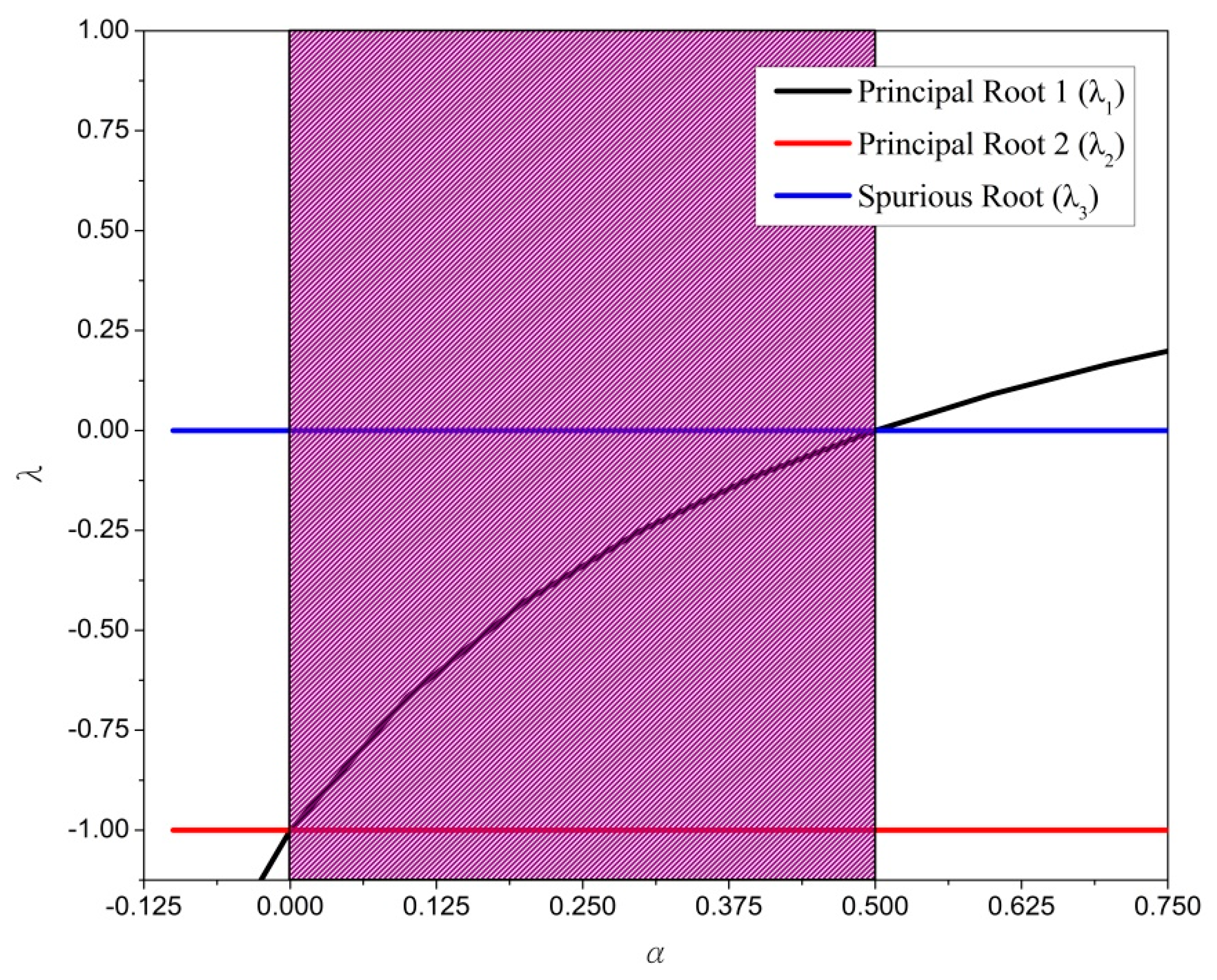
and its correspondent roots are:
In the limit
, the spurious root
only depends upon
, and
is needed so that
. On the other hand, in the limiting case of
the principal roots are functions of
and
, and it seems that the simplest way to determine the relationship between
and
leads to:
Therefore, the second line of Equation (15) determines that the two principal roots are found to be
and
in addition to
.
Figure 1 represents the variations of
and
with
This figure tells us that CVM is stable in the limit
, and reveals that the range of
is of practical interest for a linear elastic system. There is an excellent idea to simplify the stability conditions in the limit
by assuming that the roots are in terms of
that is actually a special case of the spectral radius, which is generally defined as
for the general value of
. Hence, the coefficients are found to be:
From the stability conditions, the interval range of is found to be .
5. Primary Analysis for the Nonlinear System
Chang found that an SDIM is unconditionally stable for a stiffness softening nonlinear or linear system, while it can become conditionally stable for a stiffness hardening nonlinear system. To monitor stiffness change, a parameter instantaneous degree of nonlinearity is introduced. In fact, it is defined as a ratio of the stiffness at the end of the
i-th time step over the initial stiffness, and it can be expressed as
It is clear that δi = 1 means that the instantaneous stiffness at the end of i-th time step is equal to the initial stiffness, whereas a case of instantaneous stiffness hardening δi > 1 implies that is greater than at the end of i-th time step, and a case of instantaneous stiffness softening 0 < δi < 1 inferred that the instantaneous stiffness is smaller than the initial stiffness.
6. The Stability Amplification Factor
The stability amplification factor, introduced by Chang, is used to enlarge an unconditional stability interval for an SDIM [
28]. In order to verify the unconditional stability range for CVM, a free parameter
σ is added. As a result, after including the stability amplification factor in Equation (3), the coefficients
to
and
pi+1 become:
in which:
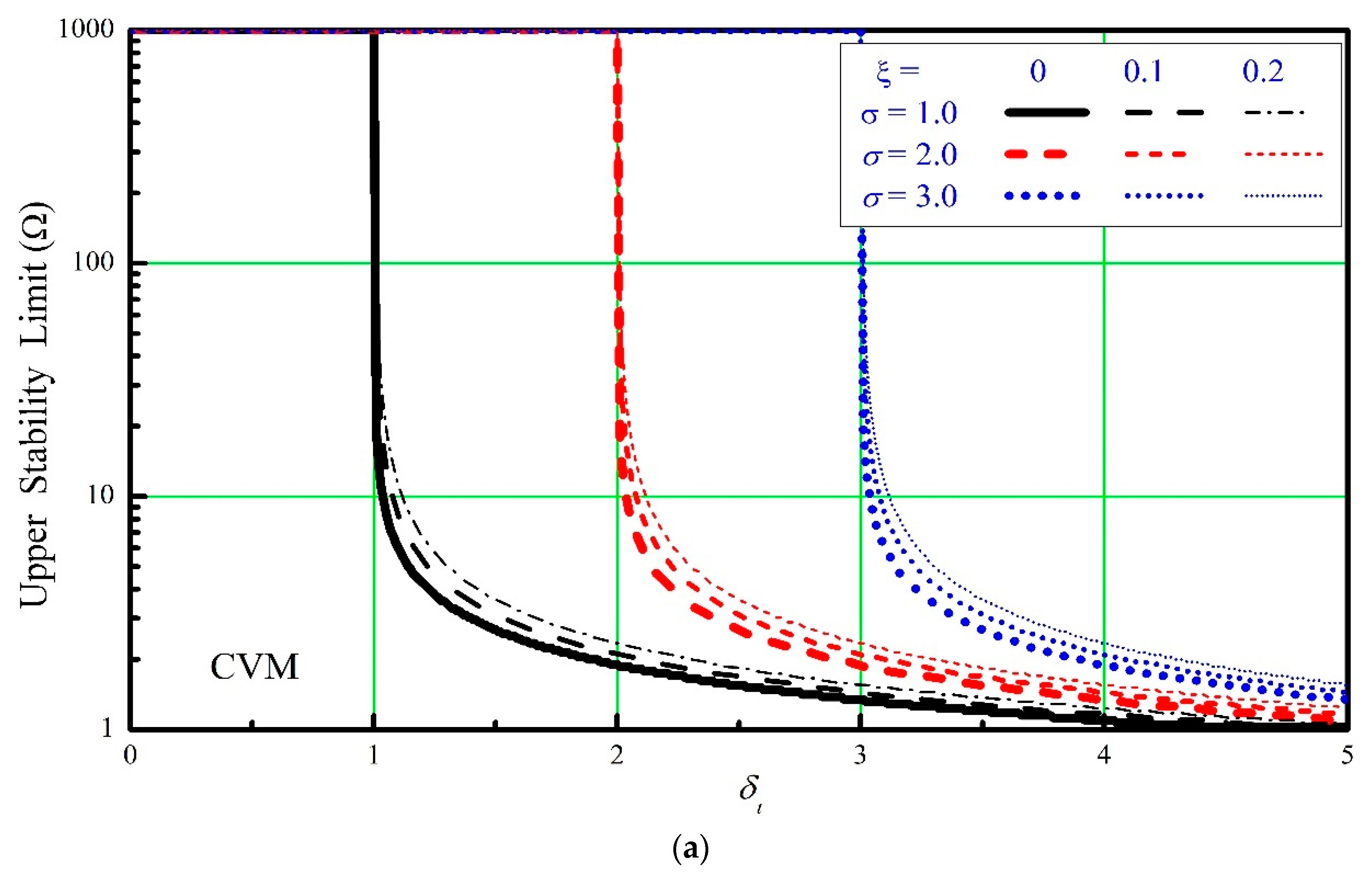
In order to verify the stability condition of CVM, with the inclusion of a free parameter
σ the upper stability limit with
is displayed in
Figure 2a,b for the different values of
, and
for the different values of the viscous damping ratios, 0, 0.1 and 0.2, respectively. The case of
implies that there is no inclusion of a free parameter of CVM. When
, CVM is unconditionally stable within the range of
and for
, CVM is unconditionally stable within the range of
. It can be understood that the large value of the stability amplification factor enlarges the unconditional stability range. However, later on in the paper, it will be shown that the larger value of
will decrease the accuracy of an integration method [
22]. Although the value of
is not known before calculation, Chang recommended that
[
20,
21,
22,
23]. In practice, it is rare to experience that real structure whose instantaneous stiffness is greater than two times of the initial stiffness, i.e.,
. In fact, the case of
is thoroughly investigated in the following study.
7. Numerical Properties of CVM
The stability amplification factor is used to enlarge the unconditional stability range of CVM. The application of this parameter is studied further for the other numerical properties of CVM. The evaluation details are referred to from references and they will not be elaborated in this paper.
7.1. Spectral Radius
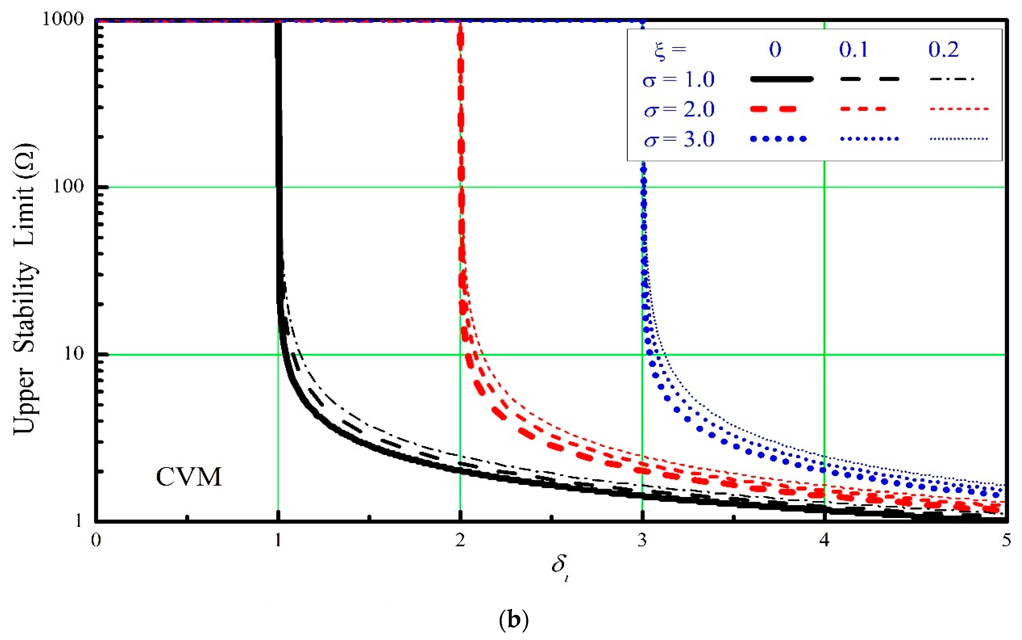
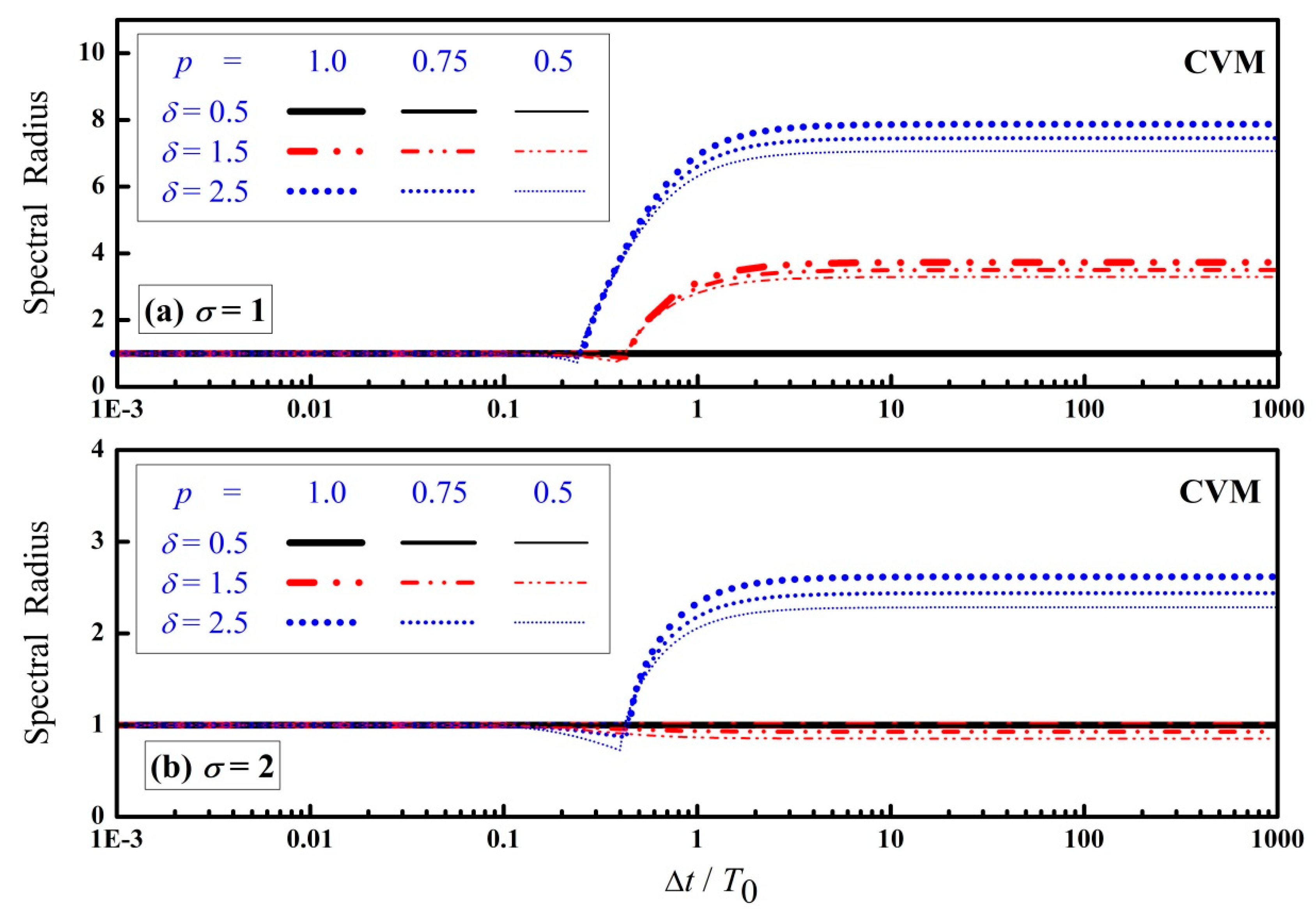
The spectral radius is used to reveal the stability of an integration method. The variation of the spectral radius with
is shown in
Figure 3, for different
and
. In general, the spectral radius is very close to 1 for the small value of
, while it decreases, step by step, and finally tends to a certain constant. In
Figure 3a,
is chosen, which means that there is no inclusion of a stability amplification factor. It shows that the spectral radii will become larger than 1 and, finally, approach a certain constant as
, after a particular value of
Figure 3b shows that the spectral radius is always less than or equal to 1 with the entire value of
for
. These results suggest that
can extend the unconditional stability range of CVM from
to
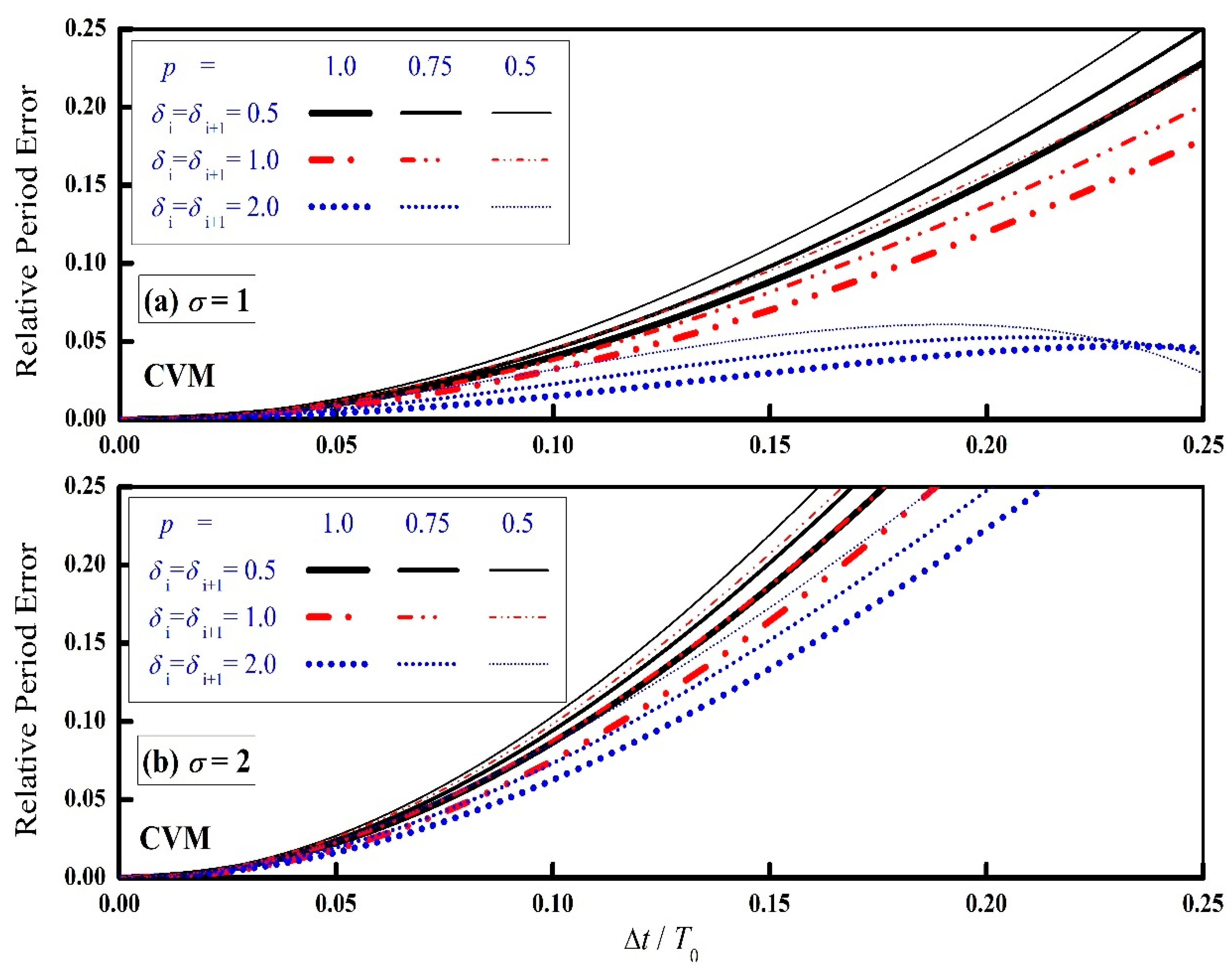
7.2. Relative Period Error
The relative period error is frequently used as a measure of period distortion for an integration method. The variation of relative period errors with
for the different values of
and
are displayed in
Figure 4. It is clear from the figure that the relative period error increases with the increase in
, as
and
are given. Comparing
Figure 4a,b, the relative period error is slightly higher for the case of
than that of case
. Even the great value of
can modify the unconditional stability range and it also results in notable period distortion; therefore, it is not suitable to select a very large value of
. For the practical application, the choice of
is good enough for the real structural system and the period distortion is acceptably small. In addition,
Figure 4 implies that, for the nonlinear system, CVM with
can generally provide an acceptable solution with comparable accuracy.
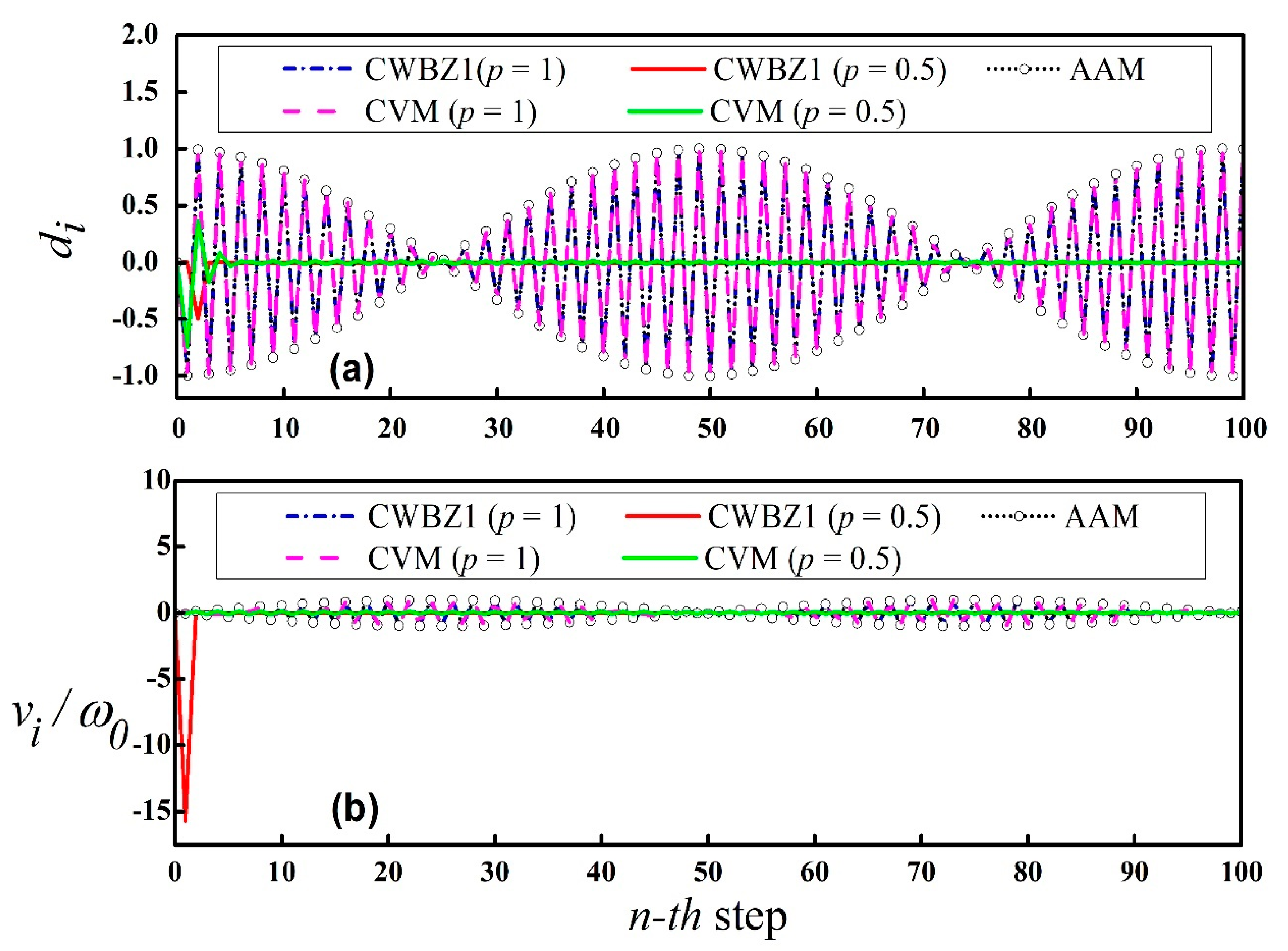
7.3. Overshooting
Goudreau and Taylor found that an integration algorithm has overshooting behavior. Later, Hilber and Hughes proposed a technique to identify such an overshoot. To determine the overshoot behavior of an integration algorithm, one can compute the velocity and discrete displacement in terms of the previous step data. In general, these results can give a sign of the high-frequency performance of the integration algorithm. A previously published Chang family method, named as CWBZ1, is considered to compare the overshoot behavior of CVM [
30]. As a result, the results for CVM and CWBZ1 for the limiting case of are found to be
From this equation, we noted that there is no overshoot behavior for any member of CVM in displacement and velocity, and CWBZ1 has no overshoot in the displacement for any value of , while it has a tendency to overshoot the quadratic in in the velocity equation due to the initial displacement term.
In order to verify the analytical prediction of the overshooting behavior of two methods, the free vibration response of the SDOF system was computed by using an almost large time step. In fact, it was computed by using CVM and CWBZ1 with
and
with a time step corresponding to
for the three initial conditions of i.
and
, ii.
and
and iii.
and
. The numerical findings are displayed in
Figure 5,
Figure 6 and
Figure 7 for the corresponding initial conditions i., ii. and iii. At the bottom of the
Figure 5b,
Figure 6b and
Figure 7b, the velocity term in the vertical axis is normalized by the natural frequency of the system (
), in order to have the same unit as displacement. For comparison, the results obtained from the constant average acceleration method (AAM) are also presented in
Figure 5,
Figure 6 and
Figure 7. It is shown that CVM exhibits no overshoot in both displacement and velocity in all three figures for
and
. In the curve for CVM
coincides with that of AAM. Similarly, it is displayed on the top plot of
Figure 5,
Figure 6 and
Figure 7 that the two curves for CWBZ1 exhibit no overshoot in displacement, as the curve for CWBZ1 with
coincides with that of AAM. Whereas the bottom part of
Figure 5b,
Figure 6b and
Figure 7b shows a significant overshoot in velocity for CWBZ1 with both
and
, although it is almost annihilated in the first few time steps for
. As a result, both analytical and numerical results prove that CVM has no overshoot in displacement and velocity, whereas CWBZ1 has no overshoot in displacement and it has a significant overshoot in velocity. As a summary, these numerical results are in good agreement with the analytical results.
8. Numerical Example
Since the introduction of the virtual parameter into CVM only alters the coefficients and the loading dependent term, the execution details of CVM for the numerical applications are almost unaffected. In addition, to confirm the numerical properties of CVM after including , the following numerical examples are carried out.
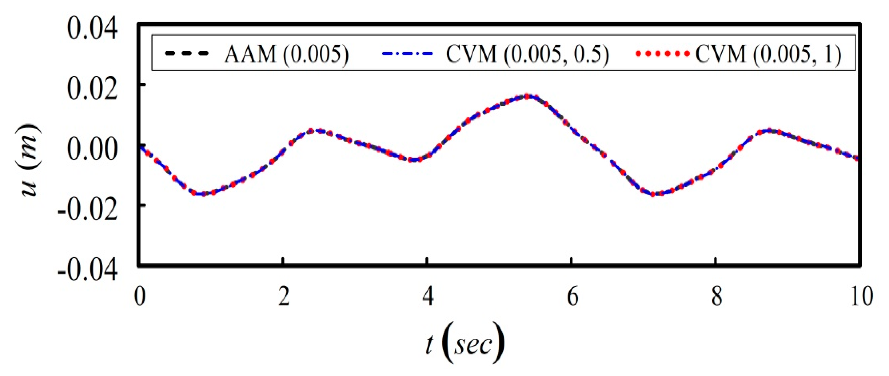
8.1. Forced Vibration Nonlinear SDOF System with Damping
A forced vibration nonlinear damped SDOF system is considered in this example. The mass and nonlinear stiffness are taken to be
and
for
. Meanwhile, the nonlinear velocity dependent damping is assumed as:
In general,
and
are generally found [
36]. In this exploration,
and
are taken. The ground acceleration is taken as
. In this numerical experiment, AAM, with the time of 0.005 s, is taken as a reference solution. CVM (0.005, 0.5) and CVM (0.005, 1) are chosen for the analysis. The displacement responses are shown in
Figure 8. The CVM results match exactly the AAM and it reveals that CVM can accurately solve nonlinear velocity-dependent problems. Hence, it is proved that the CVM can be successfully used for the velocity-dependent problem, while AAM is an implicit method.
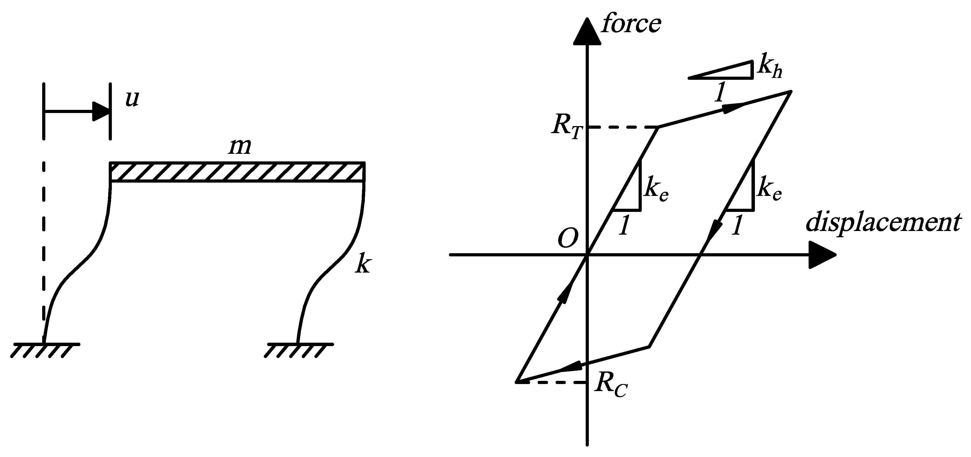
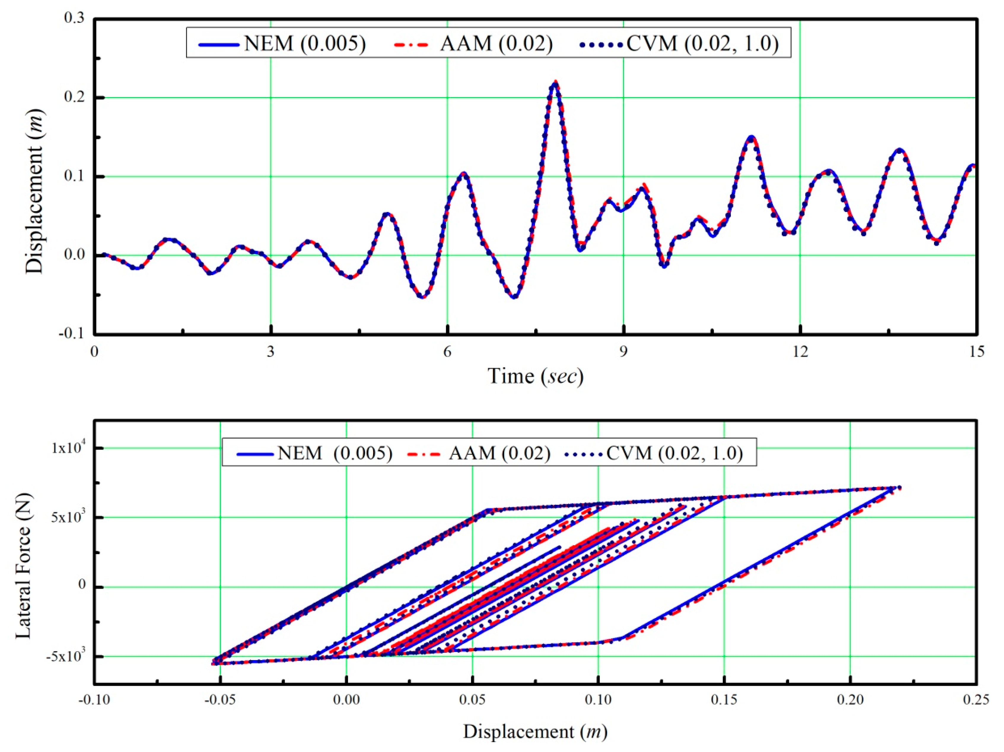
8.2. An Elastoplastic Structure
In this study, a bilinear inelastic hysteretic behavior model of SDOF is considered (
Figure 9). The lumped mass of
m = 4000 kg, the elastic stiffness of
N/m and the hardening stiffness of
N/m are assumed for the system. The initial natural frequency of the system, based on the initial structural properties, is found to be
rad/s, while the initial structural period
is 1.25 s. The yielding strength of the elastoplastic model is taken to be
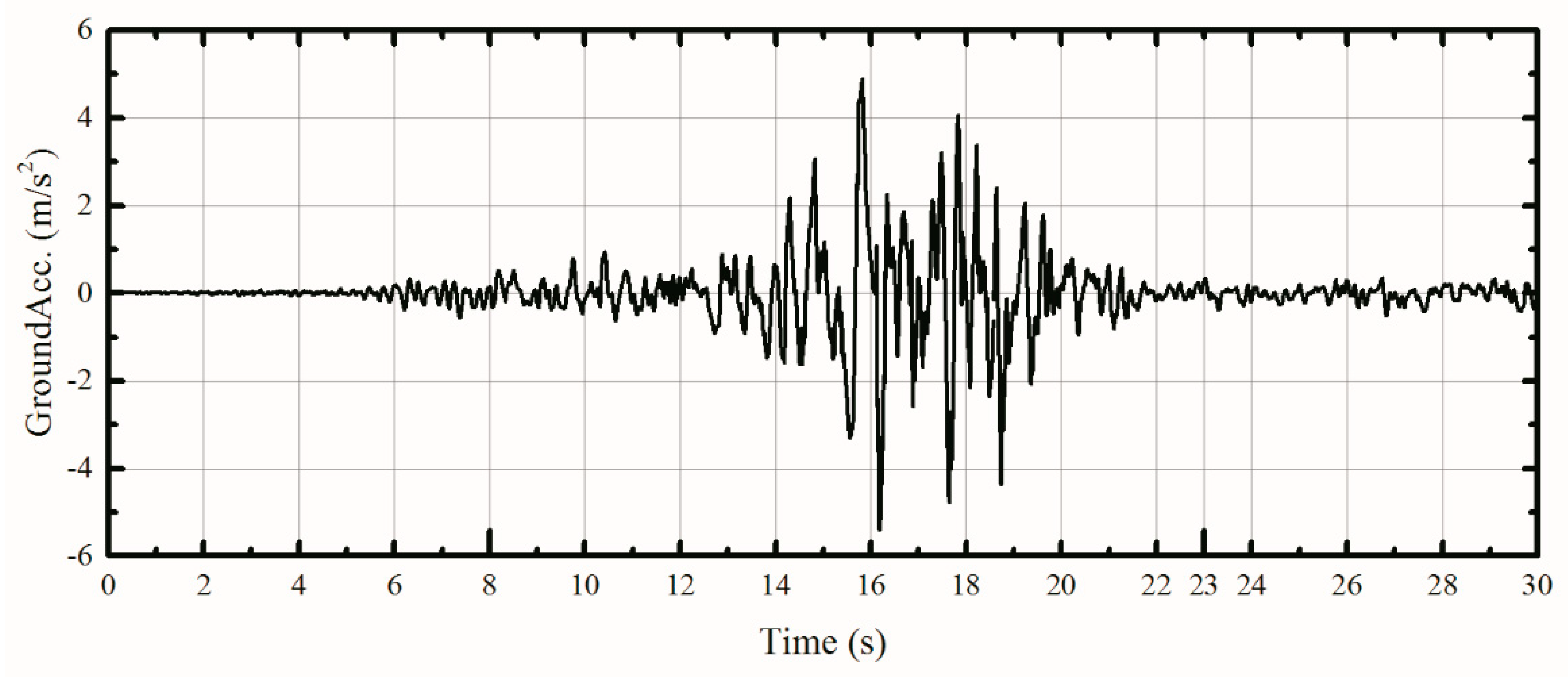
N for both the compression and tension. The undamped system is subjected to an earthquake record of CHY028 with a peak ground acceleration of 0.5 g. It should be mentioned that CHY028 is a near-fault ground motion record recorded by the Central Weather Bureau under the Taiwan Strong Motion Instrumentation Program, during the main shock of the Chi-Chi earthquake (
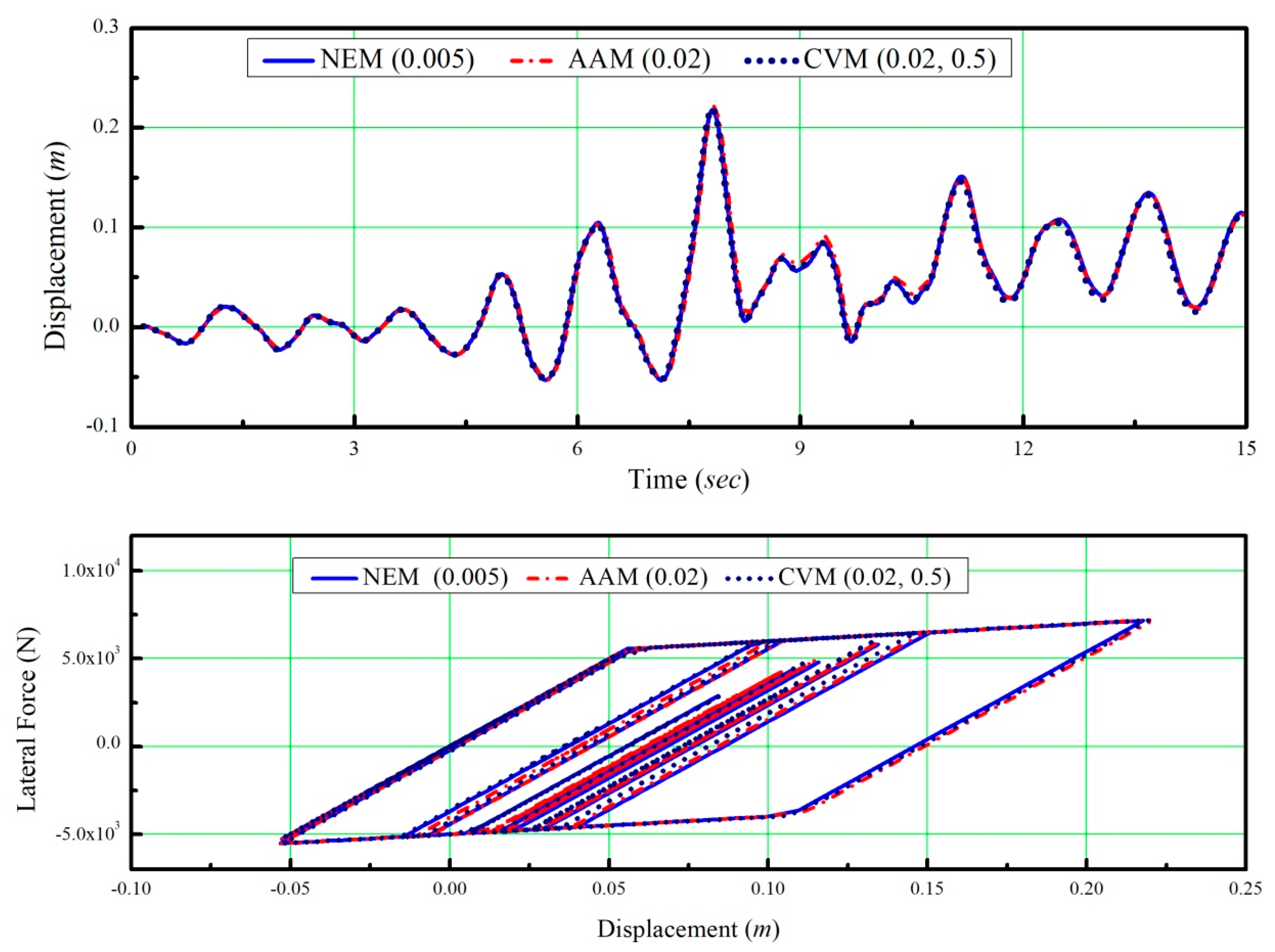
Figure 10). The numerical results are obtained for the different values of
p = 0.5 and 1, and are shown in
Figure 11 and
Figure 12, respectively. NEM (0.005), AAM (0.02), CVM (0.02, 1) and CVM (0.02, 0.5) are used in this problem. The numerical solutions obtained from NEM (0.005) are considered as the reference solutions for comparison. In the
Figure 11 and
Figure 12, the numerical solutions obtained from AAM (0.02), CVM (0.02, 0.5) and (0.02, 1) coincide with the reference solutions that are computed by NEM (0.005). As shown in
Figure 11 and
Figure 12, the system experiences highly nonlinear hysteretic behavior. The results of this example thoroughly confirm that CVM can be used to solve a highly nonlinear system.
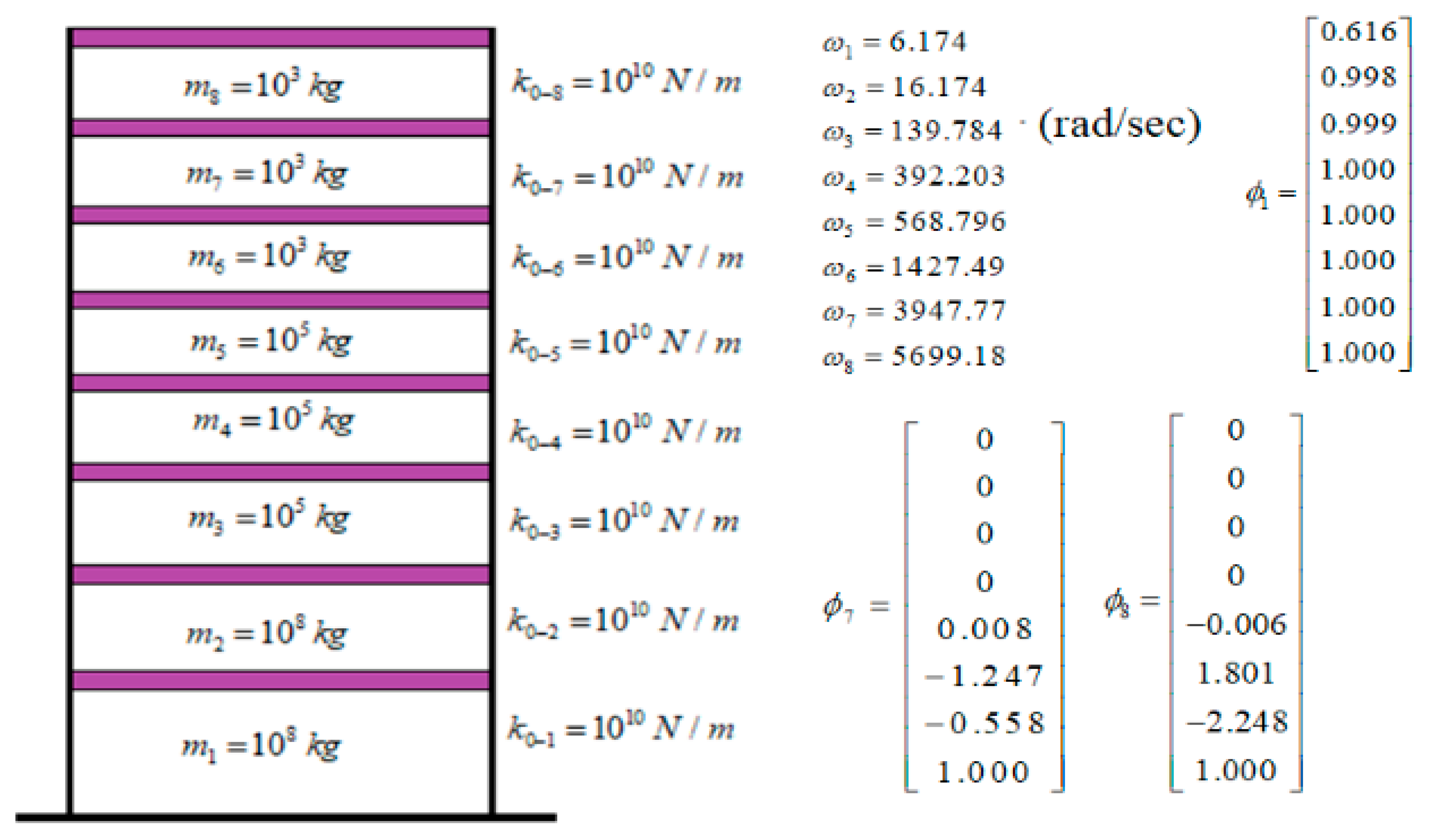
8.3. Free Vibration Responses of an Eight-Storey Building
In this example, an eight-storey shear building is examined to validate the performance of CVM. The stiffness of each story involves linear and nonlinear parts, which can be written in the form of:
where
is the instantaneous stiffness for the
i-th story. The values of
are shown in
Figure 13. A linear elastic system and a nonlinear system are simulated by specifying appropriate
q values, which are given as below
As a result, the initial natural frequencies and the 1st, 7th and 8th modal shapes of the building are given in
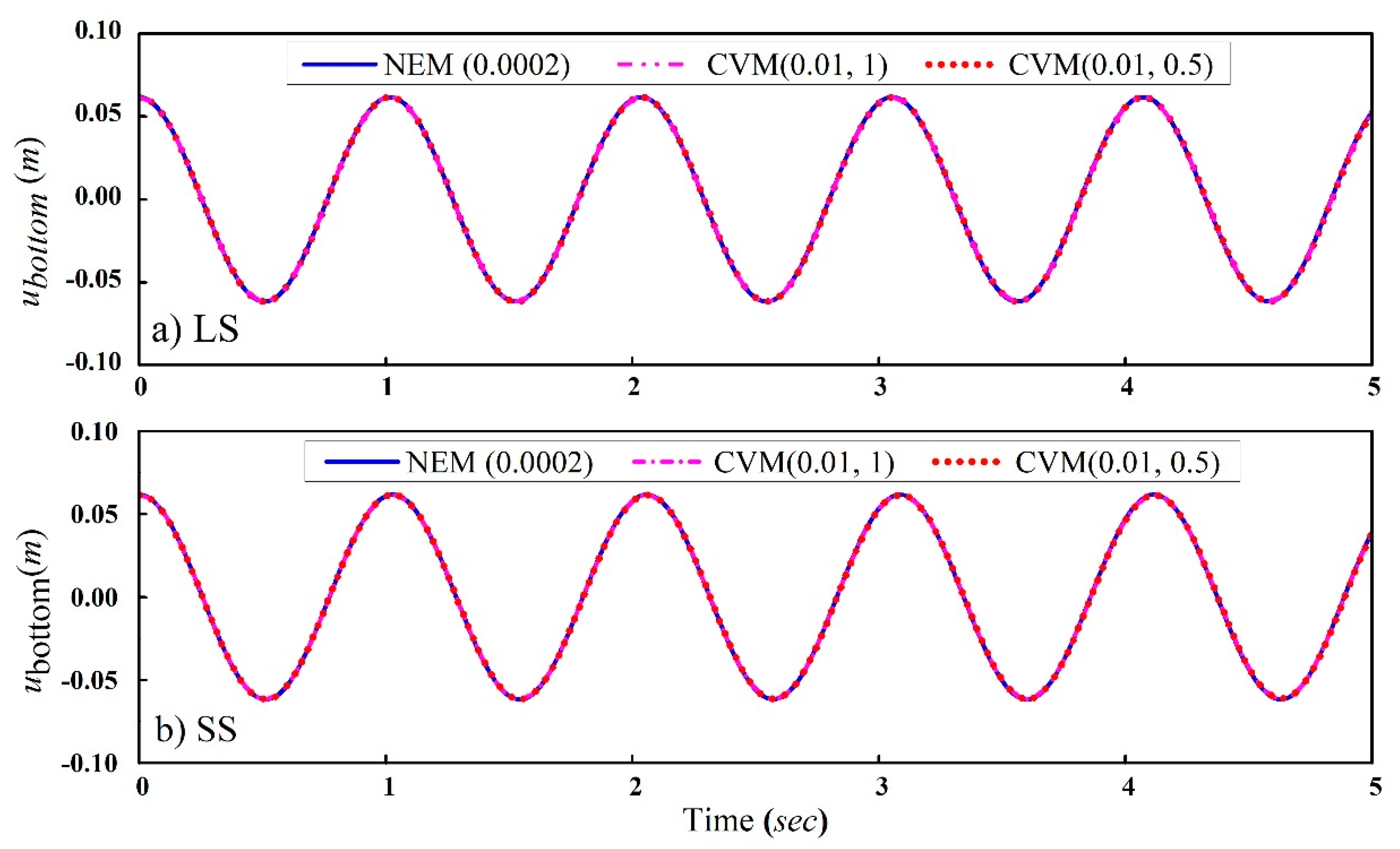
Figure 13. The initial displacement vector in Equation (25), with a zero initial velocity vector, was considered for the free vibration analysis. The free vibration responses were obtained from NEM (0.0002) and CVM (0.01) for LS and SS. The step size of NEM 0.0002 was chosen, based on the conditional stability, and it was very small. At the same time, the step size of CVM was chosen to be larger than that of NEM (i.e., 50 times). The bottom-storey responses of LS and SS are plotted and shown in
Figure 14a,b for NEM (0.0002), CVM (0.01, 0.5) and CVM (0.01, 1). From the Figure, we can see that the CVM results match the reference NEM result. It seems that the time step of 0.01 s is small enough for the CVM, for the accurate integration of the response. The results of this example confirm that CVM can be used for both linear elastic as well as the nonlinear stiffness softening system.
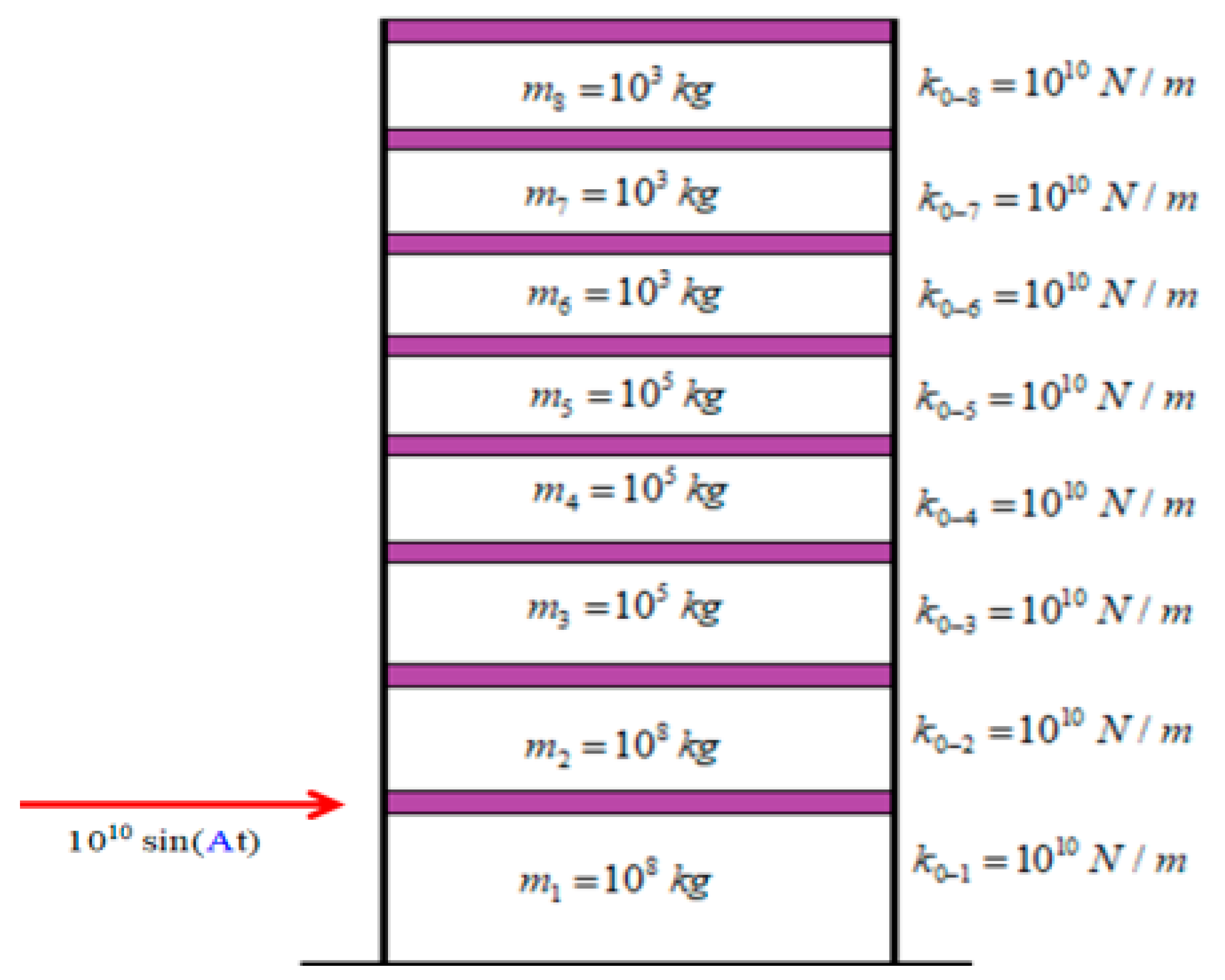
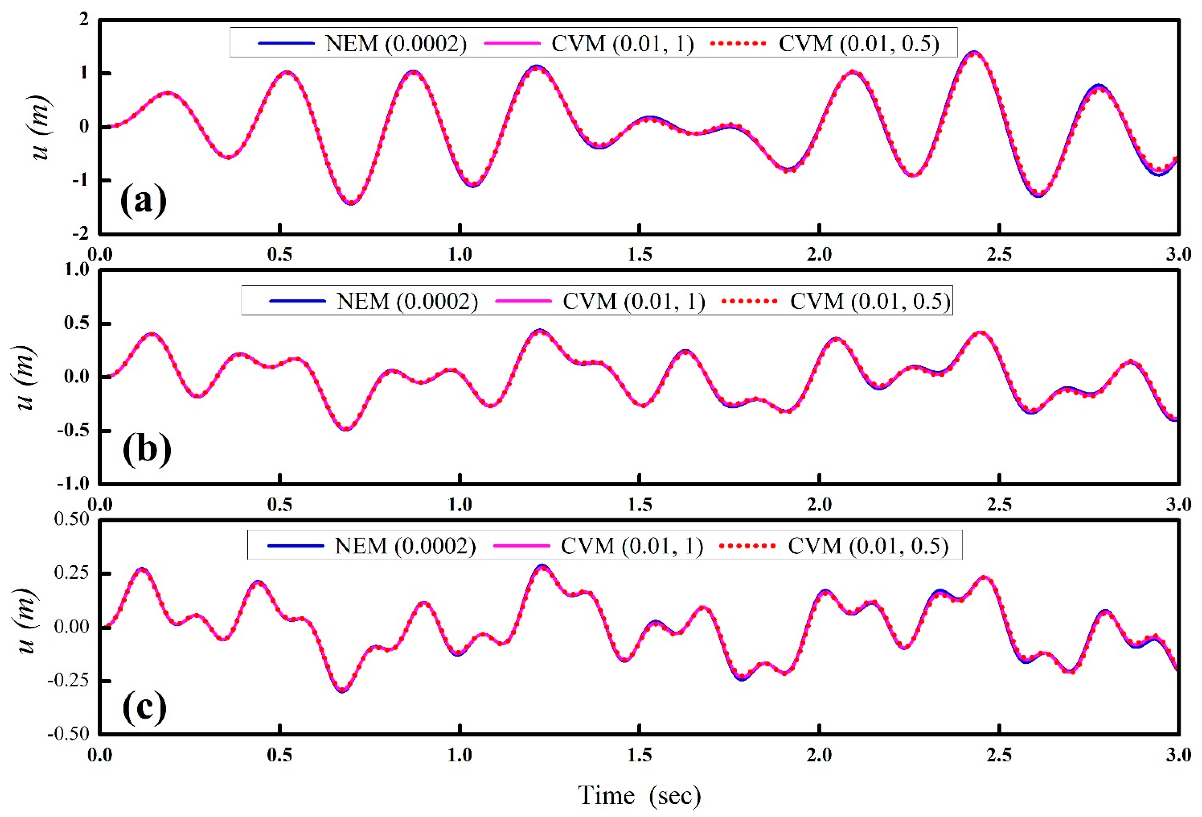
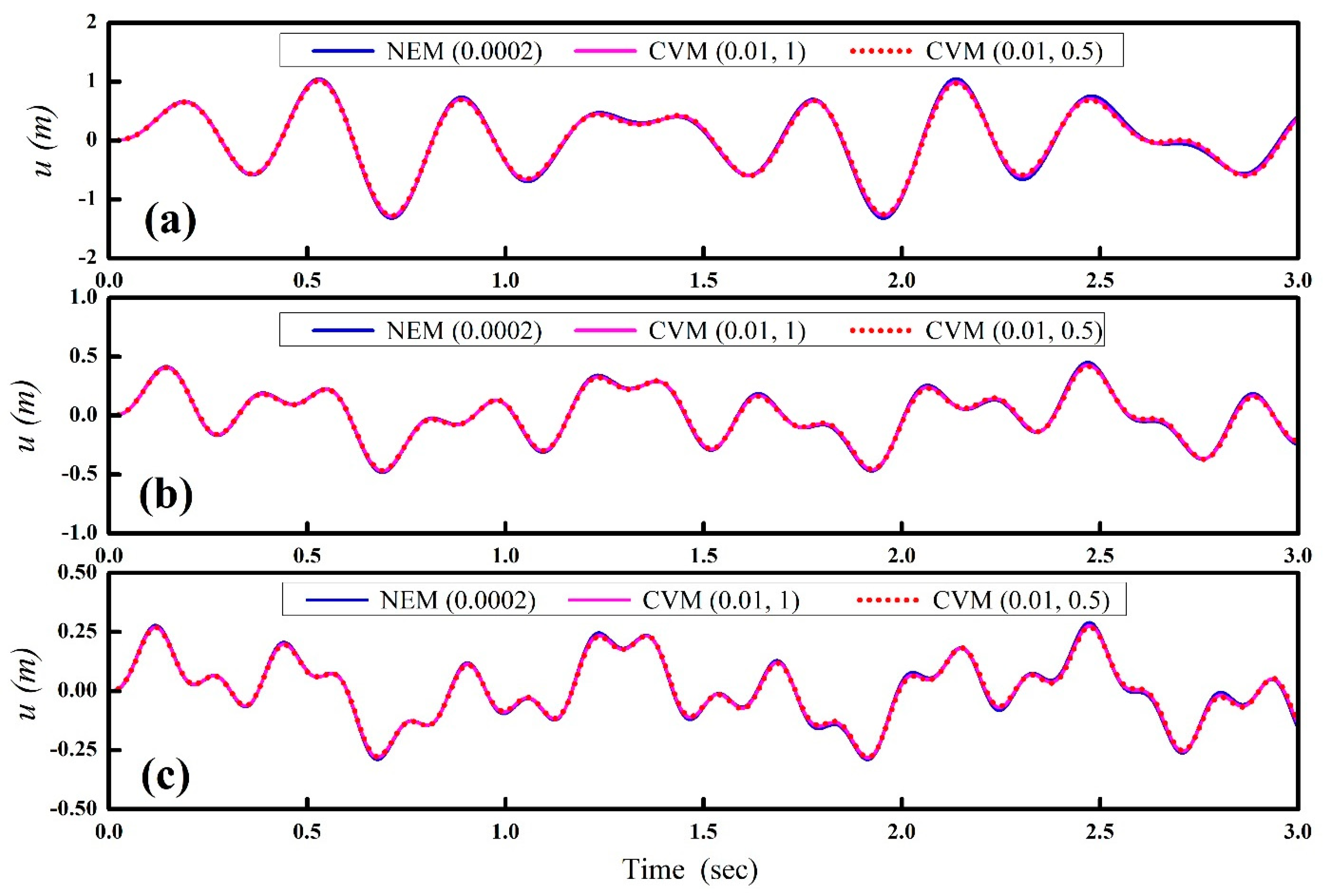
8.4. Forced Vibration Responses of the Eight-Storey Building
The same eight-storey shear beam building was considered for the analysis. In order to validate that CVM has no high frequency overshoot in a forced vibration responses, the concentrated force
N was applied on the first floor, and is shown in
Figure 15. We checked the response of the building for various
values, such as 20, 30 and 40. The NEM (0.0002) is taken as the reference solution; CVM (0.01, 0.5) and CVM (0.01, 1) are chosen for the analysis. The displacement responses of the different
values for LS and SS of the eight-storey shear building are plotted.
Figure 16a–c and
Figure 17a–c, show the forced vibration bottom-storey responses of LS and SS, for the corresponding values of
20, 30 and 40, respectively. In fact, the
values chosen for LS and SS are 0 and −0.1. These shows clearly system exhibits linear and nonlinear stiffness (softening). For both LS and SS, the results of CVM (0.01, 0.5) and CVM (0.01, 1) coincides with the reference results of NEM (0.0002). These results confirm that CVM does not have an overshoot, in high-frequency steady-state responses. In addition, the results prove that CVM can be used for linear elastics as well as nonlinear stiffness softening systems, even when the systems experience sinusoidal forces.
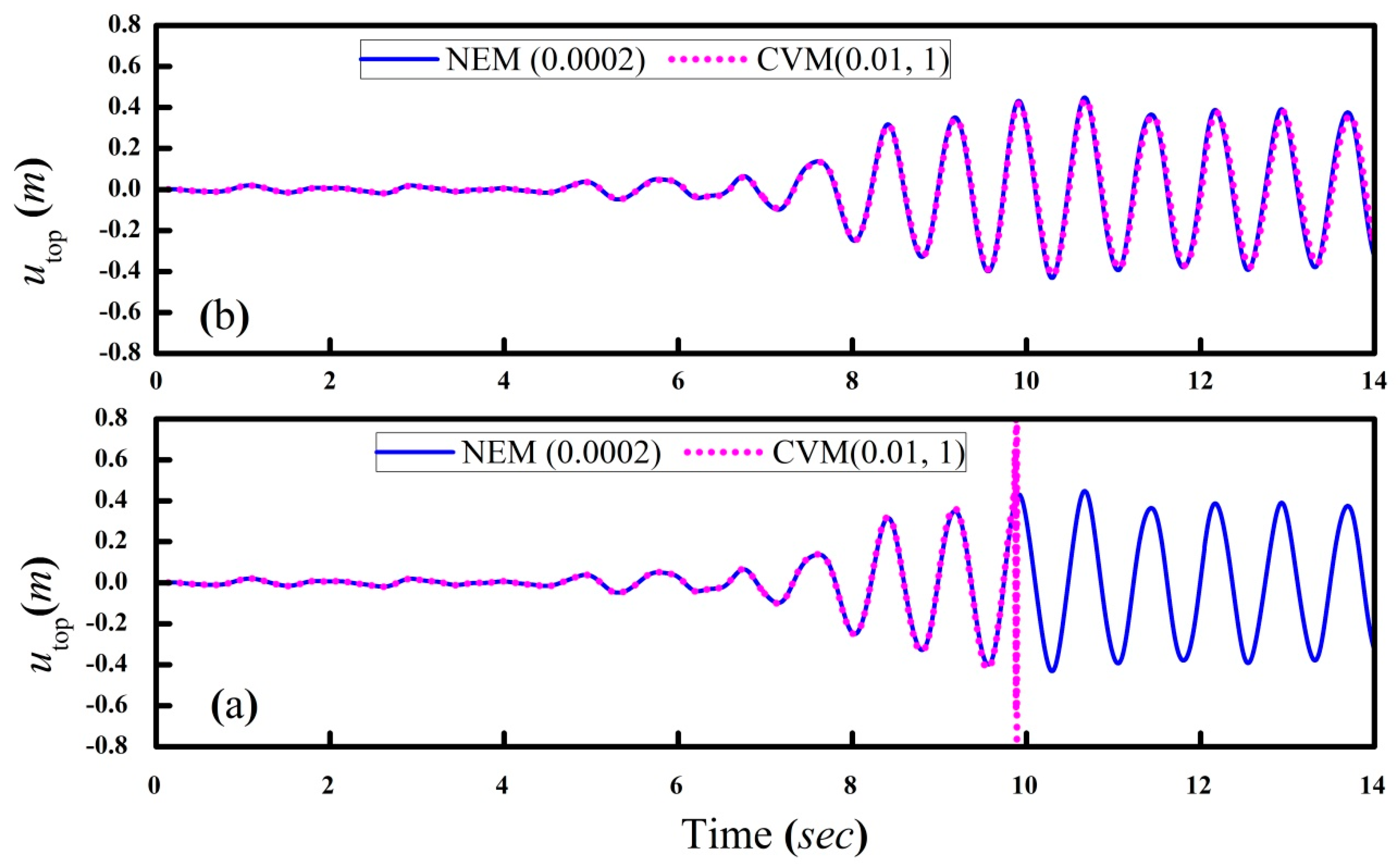
8.5. Seismic Responses of the Eight-Storey Hardening System
The same 8-DOF system is considered here for the seismic analysis. In order to attain the stiffness hardening of the system, the
q value is chosen 2. This example is very useful to show the importance of the stability amplification factor, and confirms that the CVM has unconditional stability for the stiffness hardening system. The system is subjected to the earthquake record of CHY028, with a peak ground acceleration of 0.5 g. The result of NEM (0.0002), subjected to CHY028, is considered as a reference solution. CVM (0.05, 1) is chosen for the seismic analysis. The numerical results of the top storey response are plotted in
Figure 18. In
Figure 18a, the calculated CVM (0.01, 1) displacement responses are displayed. It seems that the results are unstable. This is because HS experiences the stiffness hardening. So,
for CVM (0.01, 1) is conditionally stable for the hardening system. In
Figure 18b, the results are become stable and matches exactly with the NEM (0.0002), which exhibits the CVM (0.01, 1), with
becoming unconditionally stable. Hence, this stability amplification factor extends the CVM application for the stiffness hardening system. The results obtained from this example confirm that CVM can also be used for the nonlinear stiffness hardening system.
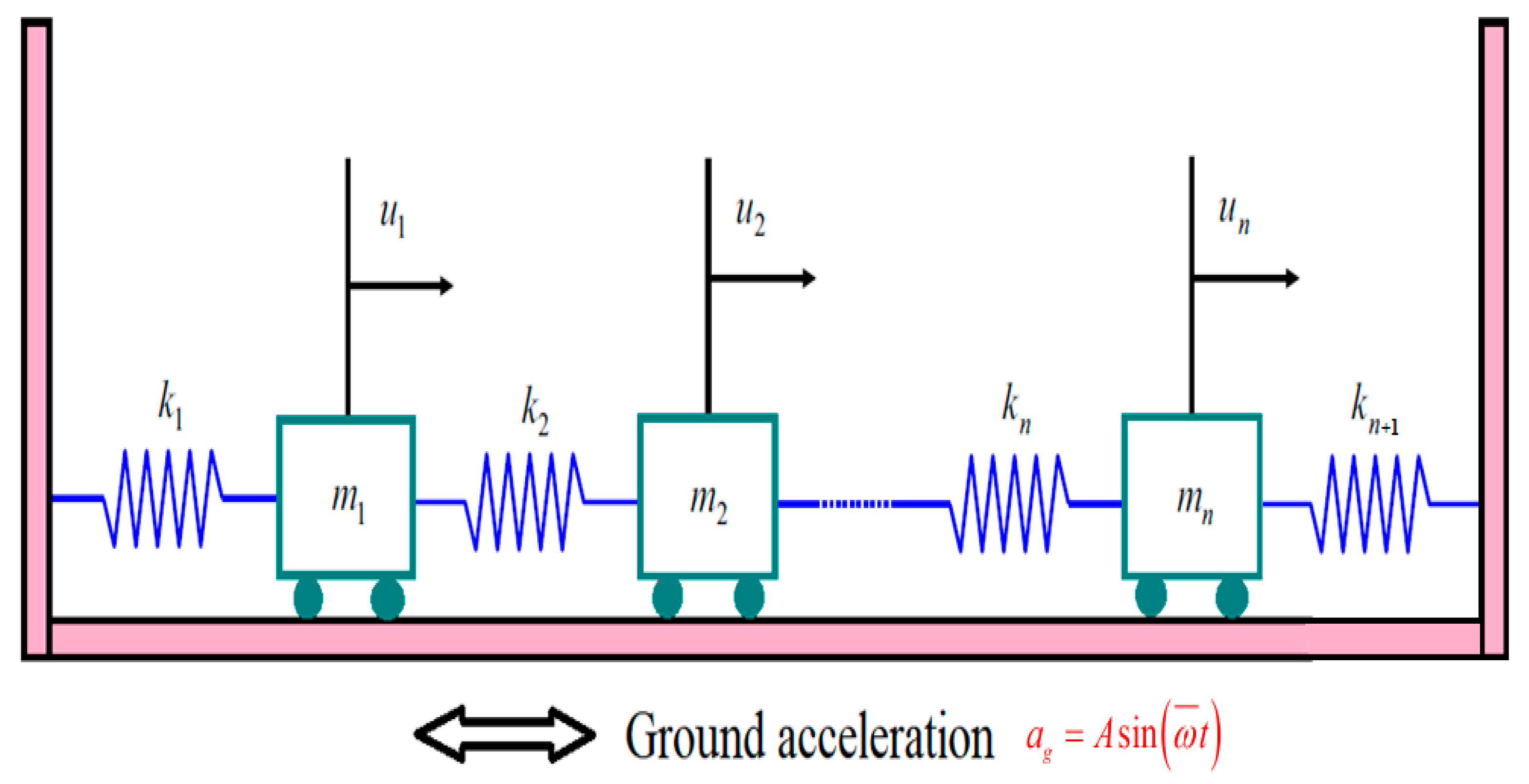
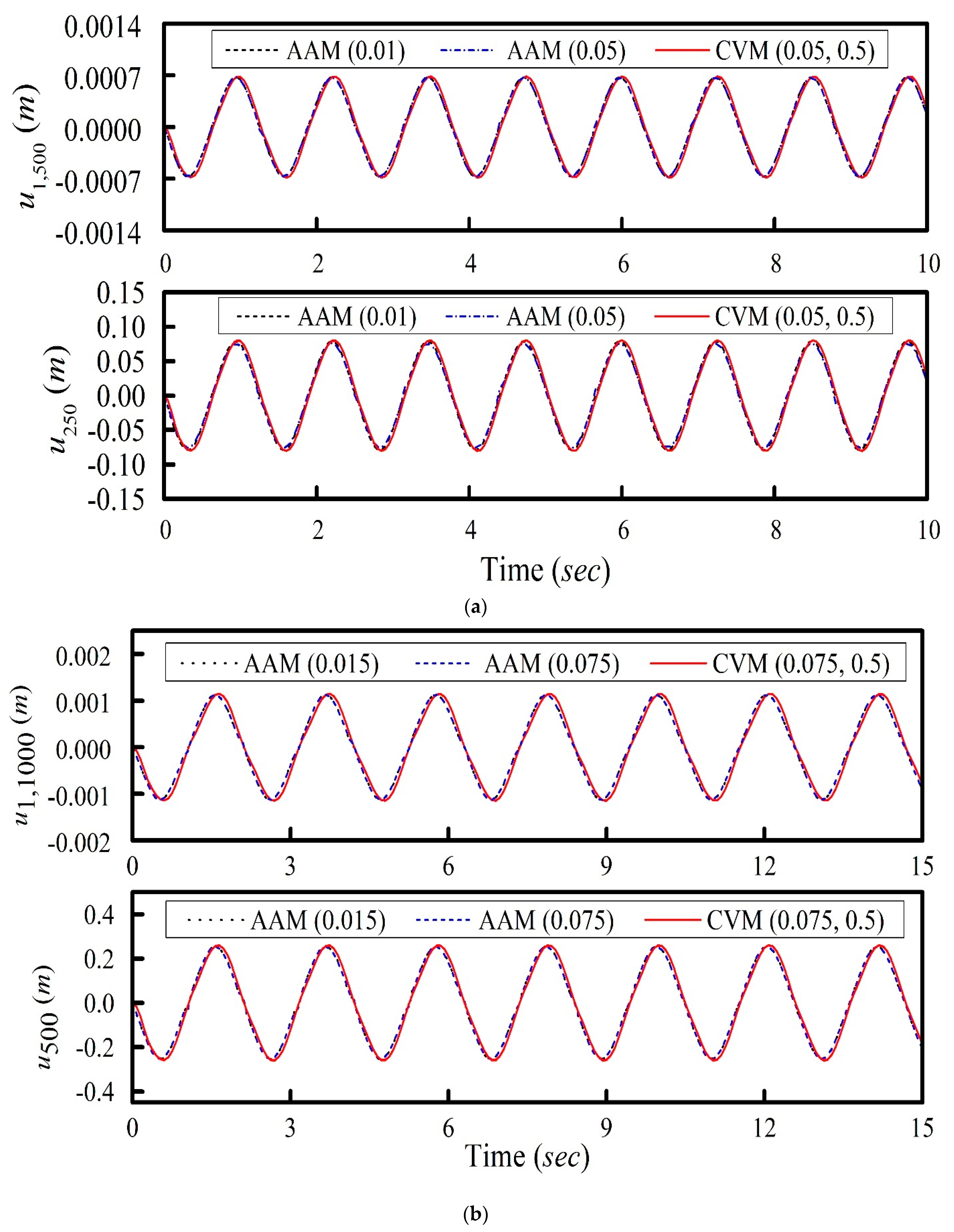
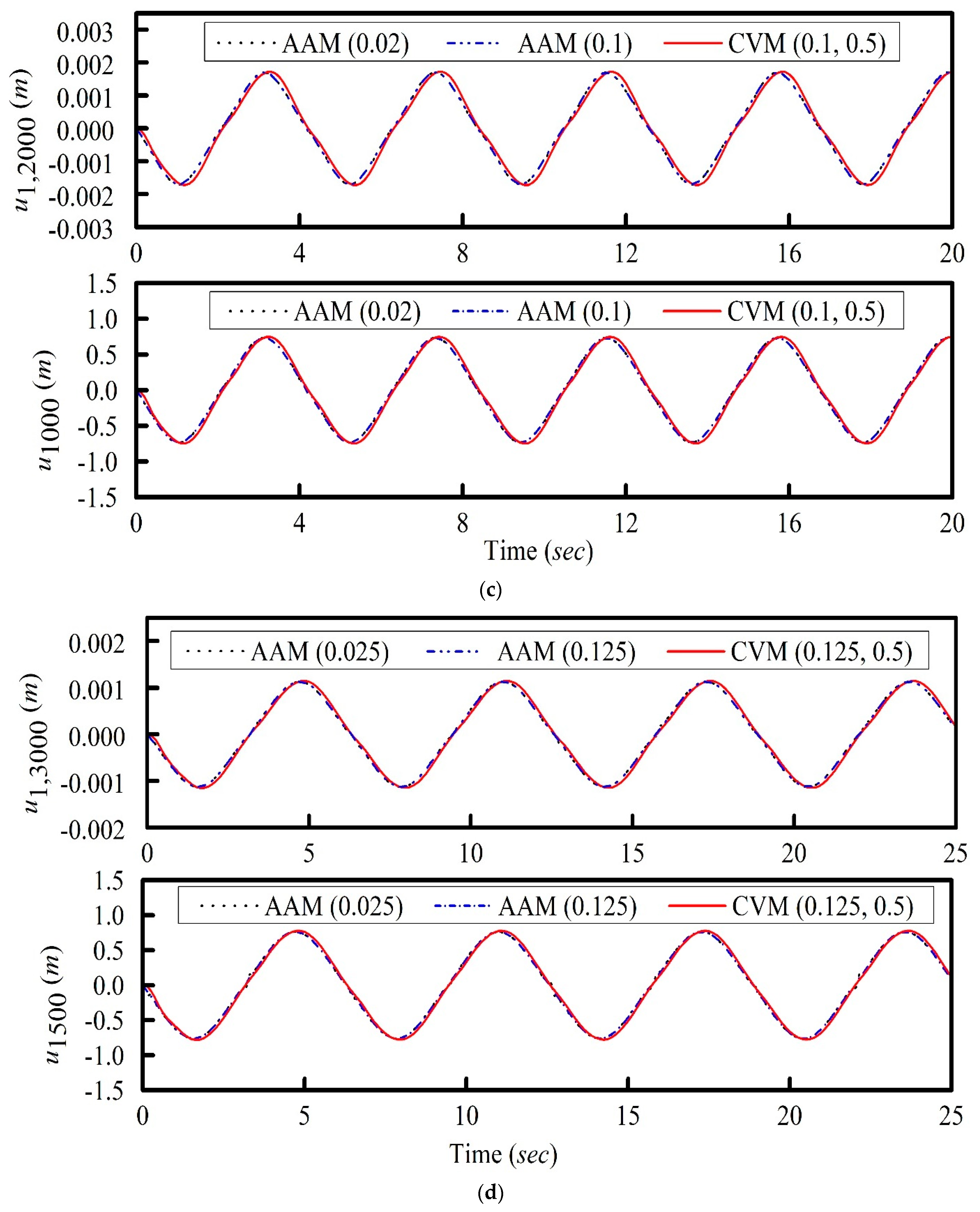
8.6. MDOF Nonlinear Mass Spring System
In this section, a series of a new mass spring system is considered and its details are shown in
Figure 19. The mass of the system is chosen as
and the stiffness is
Due to the nonlinear term, the stiffness that will decrease after deformation is assumed. In order to check the computational efficiency, the DOFs of the system are specified as
n = 500,
n = 1000,
n = 2000 and
n = 3000. The system is excited by the sin load, and the loading details are given in
Table 1. The time integration data and the lowest and highest natural frequencies of the system are given in
Table 2 and
Table 3, respectively. It is noted that the highest natural frequency is 20,000 rad/s. In this dynamic analysis, the average acceleration method (AAM) with the time steps of 0.010, 0.015, 0.020 and 0.025 are taken as the reference solution for the 500-DOF, 1000-DOF, 2000-DOF and 3000-DOF, respectively. Each analysis is carried out for a total number of 100 steps (N = 100). As a result, the two ends and center displacement responses of the system are shown in
Figure 20a–d, corresponding to the 500-DOF, 1000-DOF, 2000-DOF and 3000-DOF. It seems that the
= 0.050, 0.075, 0.100 and 0.125 s are the maximum permissible time steps to obtain the reliable solution, corresponding to the 500-DOF, 1000-DOF, 2000-DOF and 3000-DOF at the two ends and center of the new spring system.
The consumed CPU time for each nonlinear dynamic analysis is noted and listed, in
Table 4. It is seen that there is a consequential difference between the CPU time taken by AAM and CVM. This is because of nonlinear iterations are needed in each time step for AAM. However, CVM can integrate the explicit formulations and unconditional stability together. In the last column of
Table 4, R is given. It shows that R decreases with the increase of
n. It infers that the computational efficiency of the CVM will increase as the total number of DOF of the system increases.
9. Conclusions
A novel family of SDIM is proposed and, initially, it is noted that the proposed method has unconditional stability, only for linear or stiffness softening systems. A stability amplification factor is included and the stability properties of CVM are verified. As a result, the introduced free parameter can enlarge the range of unconditional stability to the nonlinear stiffness hardening system, if it is chosen to be larger than 1. In general , is strongly recommended for the proposed family method. The results of the numerical examples also prove the above condition. As a result, the stability amplification factor helps to improve the stability properties of the CVM.
The analytical and numerical results of the overshoot behavior confirm that the proposed method has no unusual overshoot behavior for the high frequency responses in both displacement and velocity to the non-zero initial conditions. The numerical example also proves that the CVM can be used for velocity dependent problems.
The unconditional stability and explicit formulations simultaneously play a key role to significantly improve the computationally efficiency of the SDIM. A new spring mass system is introduced to verify the computational efficiency of CVM. Finally, CVM has no overshoot in both displacement and velocity. Moreover, it can be applied to velocity-dependent problems and is computationally efficient where even the number of degrees of freedom increased for the new spring mass system compared with the available implicit method.
Author Contributions
Investigation, V.S.; Supervision, S.-Y.C.; Software, V.S. All authors have read and agreed to the published version of the manuscript.
Funding
Authors are grateful to acknowledge that this study was financially supported by the National Science Council, Taiwan, R.O.C., under the grant No. NSC-109-2221-E-027-002.
Institutional Review Board Statement
Not applicable.
Informed Consent Statement
Not applicable.
Data Availability Statement
Not applicable.
Conflicts of Interest
The authors declare no conflict of interest.
References
- Committee European de Normalization. Eurocode 8: Design of Structures for Earthquake Resistance, Part 1, General Rules, Seismic Actions and Rules for Buildings; European Standard; European Committee for Standardization: Brussels, Belgium, 2004. [Google Scholar]
- International Code Council. International Building Code; International Code Council Inc.: Washington, DC, USA, 2009. [Google Scholar]
- Canadian Commission on Building and Fire Codes. The National Building Code of Canada; National Research Council: Ottawa, ON, Canada, 2010. [Google Scholar]
- Newmark, N.M. A method of computation for structural dynamics. J. Eng. Mech. Div. ASCE 1959, 85, 67–94. [Google Scholar] [CrossRef]
- Goudreau, G.L.; Taylor, R.L. Evaluation of numerical integration methods in elasto-dynamics. Comput. Methods Appl. Mech. Eng. 1972, 2, 69–97. [Google Scholar] [CrossRef]
- Hilber, H.M.; Hughes, T.J.R. Collocation, dissipation and ‘overshoot’ for time integration schemes in structural dynamics. Earthq. Eng. Struct. Dyn. 1978, 6, 99–118. [Google Scholar] [CrossRef] [Green Version]
- Gui, Y.; Wang, J.T.; Jin, F.; Chen, C.; Zhou, M.X. Development of a family of explicit algorithms for structural dynamics with unconditional stability. Nonlin. Dyn. 2014, 77, 1157–1170. [Google Scholar] [CrossRef]
- Houbolt, J.C. A recurrence matrix solution for the dynamic response of elastic aircraft. J. Aeronaut. Sci. 1950, 17, 540–550. [Google Scholar] [CrossRef]
- Wilson, E.L.; Farhoomand, I.; Bathe, K.J. Nonlinear dynamic analysis of complex structures. Earthq. Eng. Struct. Dyn. 1973, 1, 241–252. [Google Scholar] [CrossRef]
- Park, K.C. An improved stiffly stable method for direct integration of nonlinear structural dynamic equations. J. Appl. Mech. 1975, 42, 464–470. [Google Scholar] [CrossRef]
- Wood, W.L.; Bossak, M.; Zienkiewicz, O.C. An alpha modification of Newmark’s method. Int. J. Numer. Methods Eng. 1981, 15, 1562–1566. [Google Scholar] [CrossRef]
- Chung, J.; Hulbert, G.M. A time integration algorithm for structural dynamics with improved numerical dissipation: The generalized-α method. J. Appl. Mech. 1993, 60, 371–375. [Google Scholar] [CrossRef]
- Chang, S.Y. Explicit pseudodynamic algorithm with unconditional stability. J. Eng. Mech. ASCE 2002, 128, 935–947. [Google Scholar] [CrossRef]
- Tamma, K.K.; Sha, D.; Zhou, X. Time discretized operators. Part 1: Towards the theoretical design of a new generation of a generalized family of unconditionally stable implicit and explicit representations of arbitrary order for computational dynamics. Comput. Methods Appl. Mech. Eng. 2003, 192, 257–290. [Google Scholar] [CrossRef]
- Zhou, X.; Tamma, K.K.; Sha, D. Design spaces, measures and metrics for evaluating quality of time operators and consequences leading to improved algorithms by design illustration to structural dynamics. Comput. Methods Appl. Mech. Eng. 2005, 64, 1841–1870. [Google Scholar] [CrossRef]
- Fung, T.C. Complex time-step Newmark methods with controllable numerical dissipation. Int. J. Numer. Methods Eng. 1998, 41, 65–93. [Google Scholar] [CrossRef]
- Kim, W.; Choi, S.Y. An improved implicit time integration algorithm: The generalized composite time integration algorithm. Comput. Struct. 2018, 196, 341–354. [Google Scholar] [CrossRef]
- Chang, S.Y. Improved explicit method for structural dynamics. J. Eng. Mech. ASCE 2007, 133, 748–760. [Google Scholar] [CrossRef]
- Chang, S.Y. An explicit method with improved stability property. Int. J. Numer. Method Eng. 2009, 77, 1100–1120. [Google Scholar] [CrossRef]
- Chang, S.Y. A new family of explicit method for linear structural dynamics. Comput. Struct. 2010, 88, 755–772. [Google Scholar] [CrossRef]
- Chang, S.Y. A family of non-iterative integration methods with desired numerical dissipation. Int. J. Numer. Method Eng. 2014, 100, 62–86. [Google Scholar] [CrossRef]
- Chang, S.Y. Family of structure-dependent explicit methods for structural dynamics. J. Eng. Mech. ASCE 2014, 140, 06014005. [Google Scholar] [CrossRef]
- Chang, S.Y. Dissipative, non-iterative integration algorithms with unconditional stability for mildly nonlinear structural dynamics. Nonlinear Dyn. 2015, 79, 1625–1649. [Google Scholar] [CrossRef]
- Chen, C.; Ricles, J.M. Development of direct integration algorithms for structural dynamics using discrete control theory. J. Eng. Mech. ASCE. 2008, 134, 676–683. [Google Scholar] [CrossRef]
- Tang, Y.; Lou, M.L. New unconditionally stable explicit integration algorithm for real-time hybrid testing. J. Eng. Mech. ASCE 2017, 143, 04017029. [Google Scholar] [CrossRef]
- Chang, S.Y. Performances of non-dissipative structure-dependent integration methods. Struct. Eng. Mech. 2018, 65, 91–98. [Google Scholar]
- Chang, S.Y. Choices of structure-dependent pseudodynamic algorithms. J. Eng. Mech. ASCE 2019, 145, 04019029. [Google Scholar] [CrossRef]
- Chang, S.Y. A general technique to improve stability property for a structure-dependent integration method. Struct. Eng. Mech. 2015, 101, 653–669. [Google Scholar] [CrossRef]
- Chang, S.Y.; Tran, N.C.; Wu, T.H. A Parameter to improve stability for a family of dissipative integration methods. J. Chin. Inst. Eng. 2016, 39, 686–694. [Google Scholar] [CrossRef]
- Chang, S.Y.; Tran, N.C.; Wu, T.H.; Yang, Y.S. A one-parameter controlled dissipative unconditionally stable explicit algorithm for time history analysis. Sci. Iranica. 2017, 24, 2307–2319. [Google Scholar] [CrossRef] [Green Version]
- Vaiana, N.; Sessa, S.; Marmo, F.; Rosati, L. Nonlinear dynamic analysis of hysteretic mechanical systems by combining a novel rate-independent model and an explicit time integration method. Nonlinear Dyn. 2019, 98, 2879–2901. [Google Scholar] [CrossRef]
- Chang, S.Y. An Eigen-based theory for structure-dependent integration methods for nonlinear dynamic analysis. Int. J. Struct. Stab. Dyn. 2020, 20, 2050130. [Google Scholar] [CrossRef]
- Vaiana, N.; Capuano, R.; Sessa, S.; Marmo, F.; Rosati, L. Nonlinear dynamic analysis of seismically base-isolated structures by a novel OpenSees hysteretic material model. Appl. Sci. 2021, 11, 900. [Google Scholar] [CrossRef]
- Clough, R.; Penzien, J. Dynamics of Structures, 3rd ed.; Computers & Structures Inc.: Berkeley, CA, USA, 2010. [Google Scholar]
- Lax, P.; Richmyer, R. Survey of the stability of linear difference equations. Commun. Pure Appl. Math. 1956, 9, 267–293. [Google Scholar] [CrossRef]
- Citterio, M.; Talamo, R. Damped oscillators: A continuous model for velocity dependent drag. Comput. Math. Appl. 2010, 59, 352–359. [Google Scholar] [CrossRef] [Green Version]
Figure 1.
Variations of the eigenvalues of A with as tends to infinity.
Figure 1.
Variations of the eigenvalues of A with as tends to infinity.
Figure 2.
Variation of upper stability limit with , (a) and (b) .
Figure 2.
Variation of upper stability limit with , (a) and (b) .
Figure 3.
Variation of the spectral radius with .
Figure 3.
Variation of the spectral radius with .
Figure 4.
Variation of the relative period error with .
Figure 4.
Variation of the relative period error with .
Figure 5.
Comparison of the overshoot response of CVM for the first initial conditions.
Figure 5.
Comparison of the overshoot response of CVM for the first initial conditions.
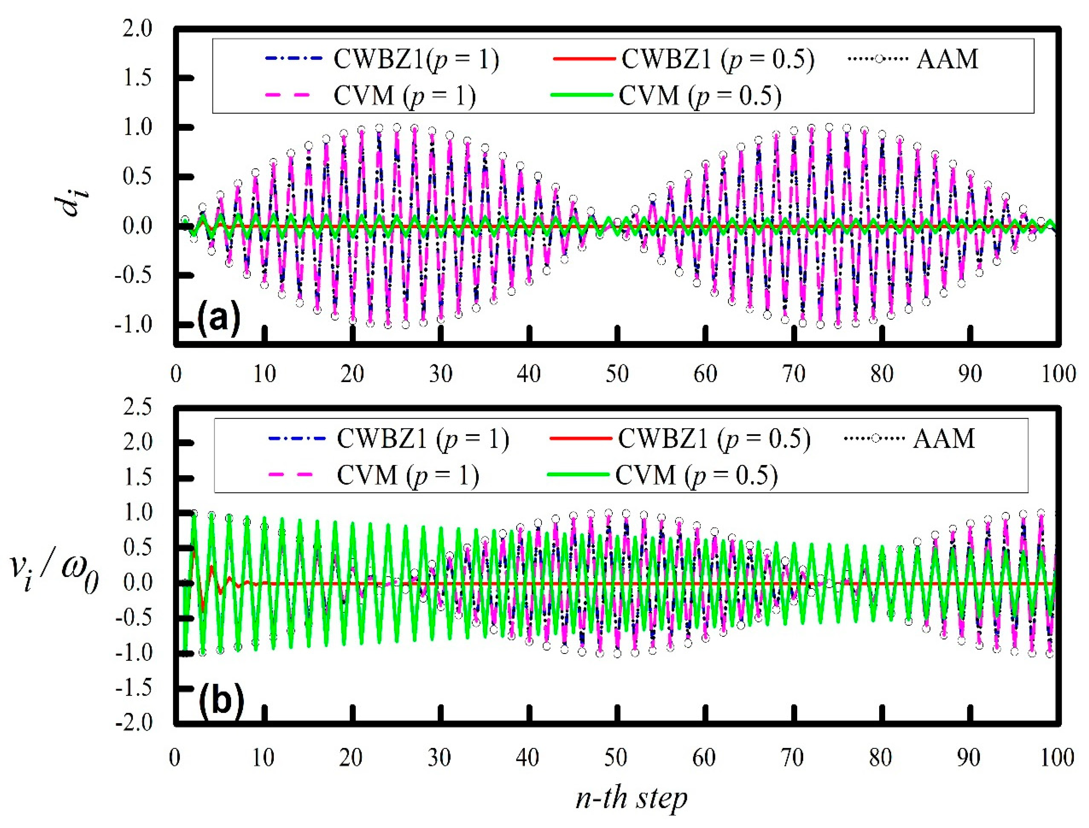
Figure 6.
Comparison of the overshoot response of CVM for the second initial conditions.
Figure 6.
Comparison of the overshoot response of CVM for the second initial conditions.
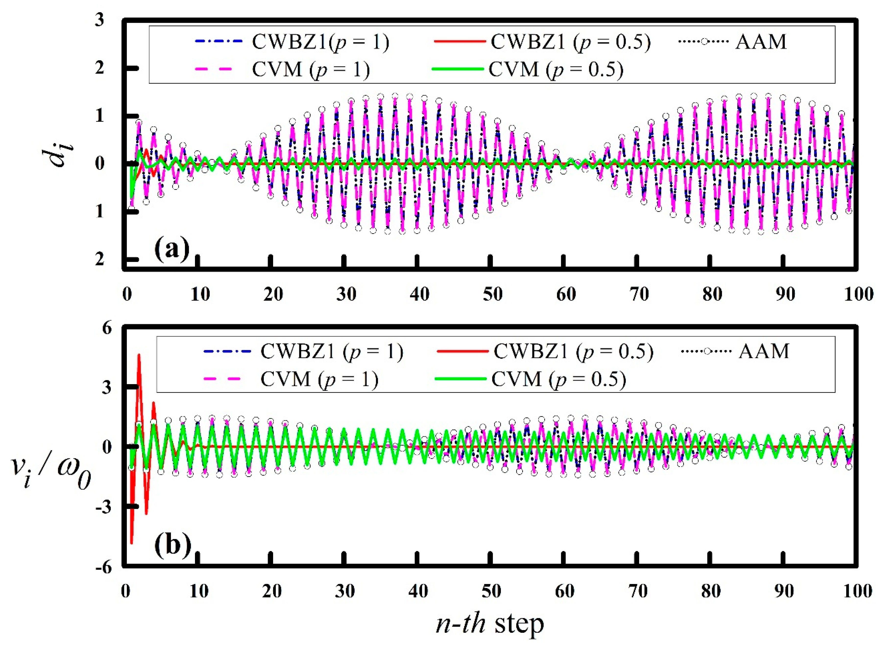
Figure 7.
Comparison of the overshoot response of CVM for the third initial conditions.
Figure 7.
Comparison of the overshoot response of CVM for the third initial conditions.
Figure 8.
Displacement response for the nonlinear damped SDOF system.
Figure 8.
Displacement response for the nonlinear damped SDOF system.
Figure 9.
An SDOF with a bilinear inelastic behavior.
Figure 9.
An SDOF with a bilinear inelastic behavior.
Figure 10.
The ground acceleration record of CHY028.
Figure 10.
The ground acceleration record of CHY028.
Figure 11.
Displacement responses to CHY028 and the corresponding hysteretic loops for .
Figure 11.
Displacement responses to CHY028 and the corresponding hysteretic loops for .
Figure 12.
Displacement responses to CHY028 and the corresponding hysteretic loops for .
Figure 12.
Displacement responses to CHY028 and the corresponding hysteretic loops for .
Figure 13.
Eight-storey shear beam building.
Figure 13.
Eight-storey shear beam building.
Figure 14.
Bottom-storey responses of the eight-storey building under free vibration.
Figure 14.
Bottom-storey responses of the eight-storey building under free vibration.
Figure 15.
Eight-storey shear beam building with external force.
Figure 15.
Eight-storey shear beam building with external force.
Figure 16.
Forced vibration bottom-storey responses of the eight-storey building for LS with different A values (a) 20; (b) 30 and (c) 40.
Figure 16.
Forced vibration bottom-storey responses of the eight-storey building for LS with different A values (a) 20; (b) 30 and (c) 40.
Figure 17.
Forced vibration bottom-storey responses of the eight-storey building for SS with different A values (a) 20; (b) 30 and (c) 40.
Figure 17.
Forced vibration bottom-storey responses of the eight-storey building for SS with different A values (a) 20; (b) 30 and (c) 40.
Figure 18.
Seismic responses of the top-storey of the eight-storey building subjected to the earthquake record CHY028 (a) (b) .
Figure 18.
Seismic responses of the top-storey of the eight-storey building subjected to the earthquake record CHY028 (a) (b) .
Figure 19.
A new mass spring system.
Figure 19.
A new mass spring system.
Figure 20.
Displacement responses for the spring mass system: (a) 500-DOF, (b) 1000-DOF, (c) 2000-DOF and (d) 3000-DOF.
Figure 20.
Displacement responses for the spring mass system: (a) 500-DOF, (b) 1000-DOF, (c) 2000-DOF and (d) 3000-DOF.
Table 1.
Ground acceleration.
Table 1.
Ground acceleration.
| N-DOF | |
|---|
| 500 | |
| 1000 | |
| 2000 | |
| 3000 | |
Table 2.
Time integration data.
Table 2.
Time integration data.
| N-DOF | |
| | N |
|---|
| 500 | 0.05 | 0.010 | 10 | 200 |
| 1000 | 0.075 | 0.015 | 15 | 200 |
| 2000 | 0.100 | 0.020 | 20 | 200 |
| 3000 | 0.125 | 0.025 | 25 | 200 |
Table 3.
Initial and highest natural frequencies.
Table 3.
Initial and highest natural frequencies.
| N-DOF | | |
|---|
| 500 | 62.71 | 20,000 |
| 1000 | 31.38 | 20,000 |
| 2000 | 15.70 | 20,000 |
| 3000 | 10.47 | 20,000 |
Table 4.
Time integration data.
Table 4.
Time integration data.
| N-DOF | CPU(AAM) | CPU(CVM) | |
|---|
| 500 | 74.59 | 1.73 | 0.023 |
| 1000 | 288.02 | 6.29 | 0.022 |
| 2000 | 1262.46 | 21.99 | 0.017 |
| 3000 | 3195.88 | 52.06 | 0.016 |
| Publisher’s Note: MDPI stays neutral with regard to jurisdictional claims in published maps and institutional affiliations. |
© 2021 by the authors. Licensee MDPI, Basel, Switzerland. This article is an open access article distributed under the terms and conditions of the Creative Commons Attribution (CC BY) license (https://creativecommons.org/licenses/by/4.0/).


