
MLGen: Generative Design Framework Based on Machine Learning and Topology Optimization


Abstract
:1. Introduction
2. Topology Optimization
2.1. Problem Formulation
2.2. The Solid Isotropic Material with Penalization (SIMP) Approach
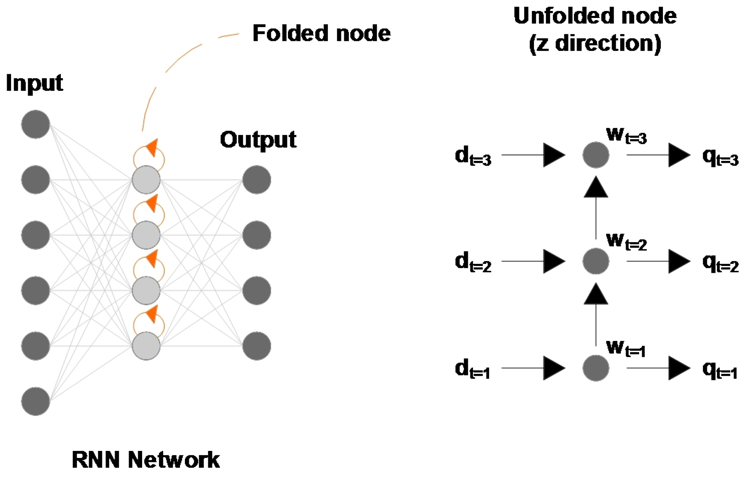
3. Long Short-Term Memory Networks
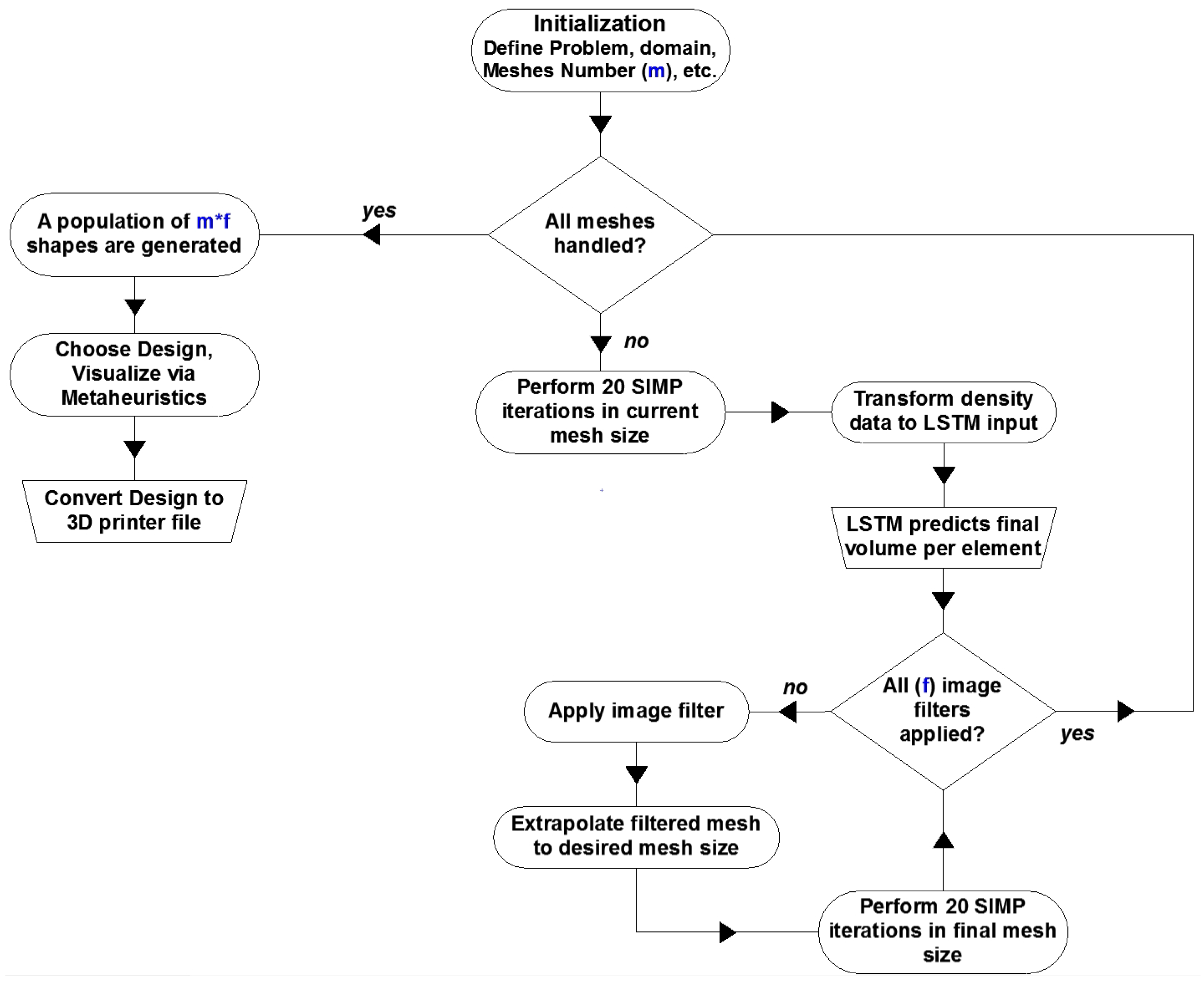
4. The MLGen Framework Description
4.1. Framework Architecture
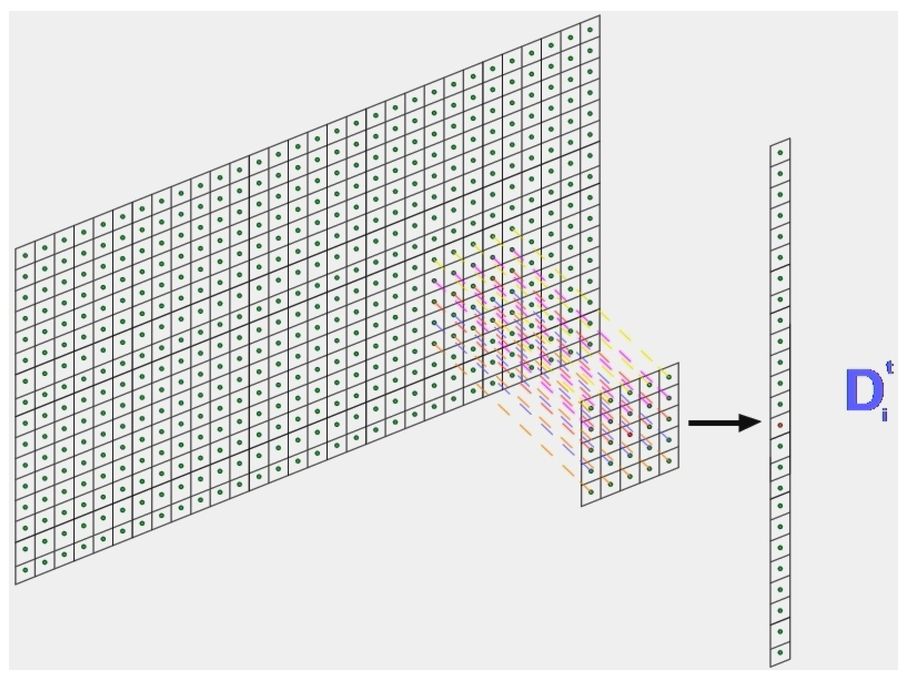
4.2. Design and Training of the LSTM Network
4.2.1. Metaheuristics
4.2.2. 3D Printing of MLGen Output
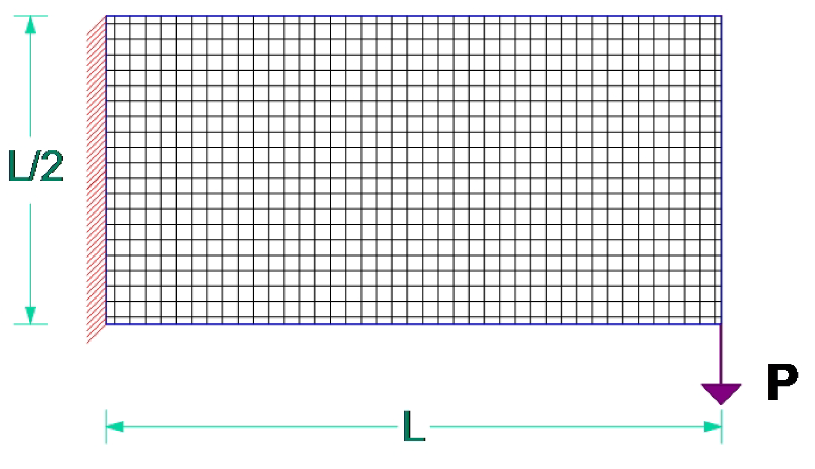
5. Numerical Tests
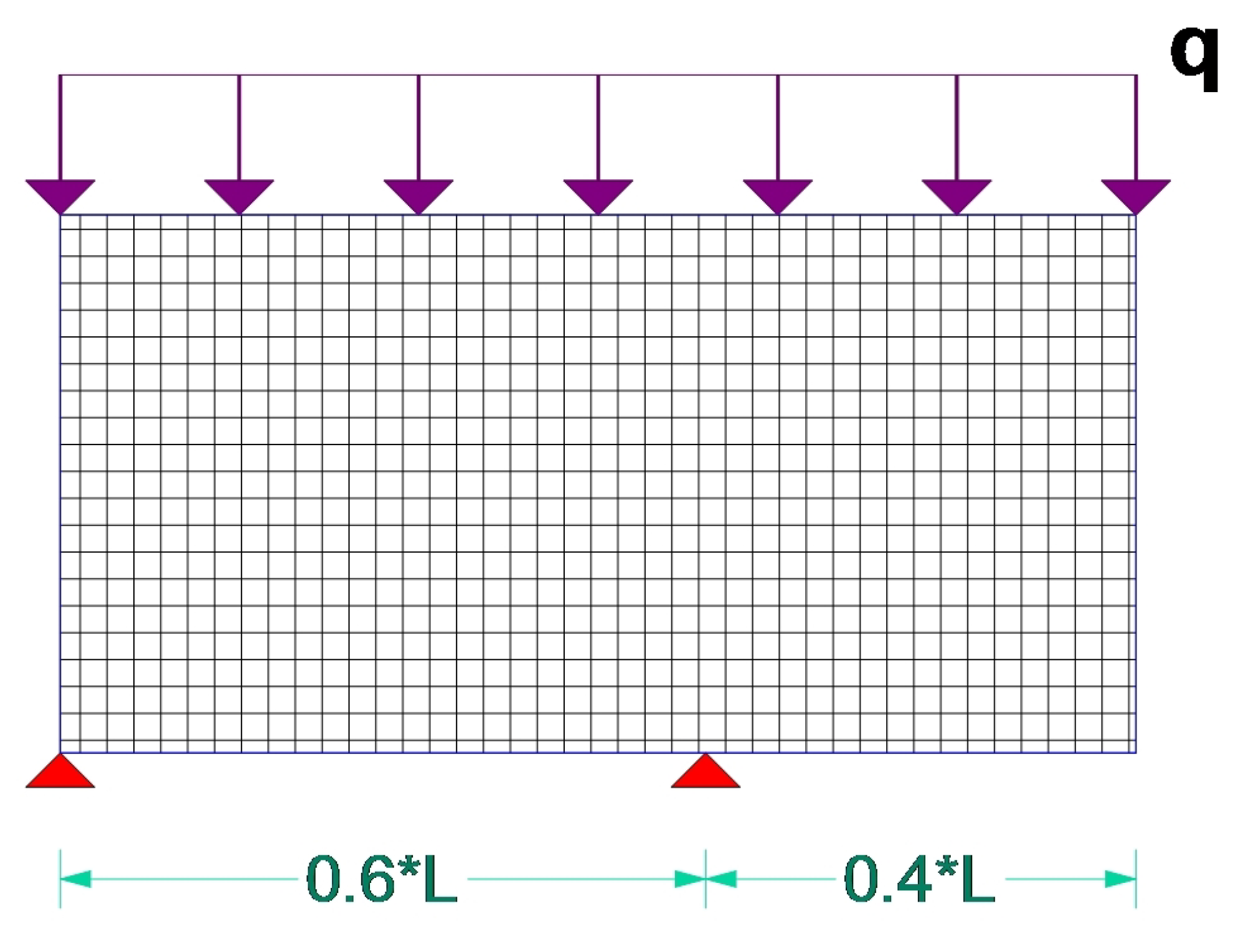
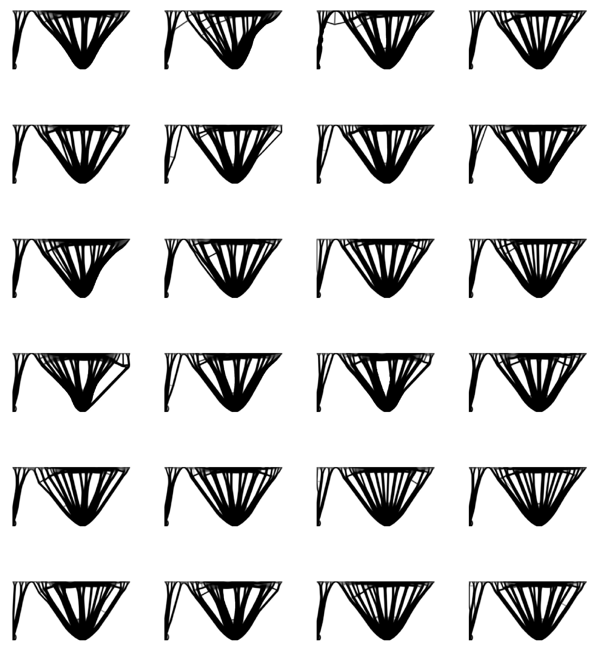
5.1. Test Example A
5.2. Test Example B
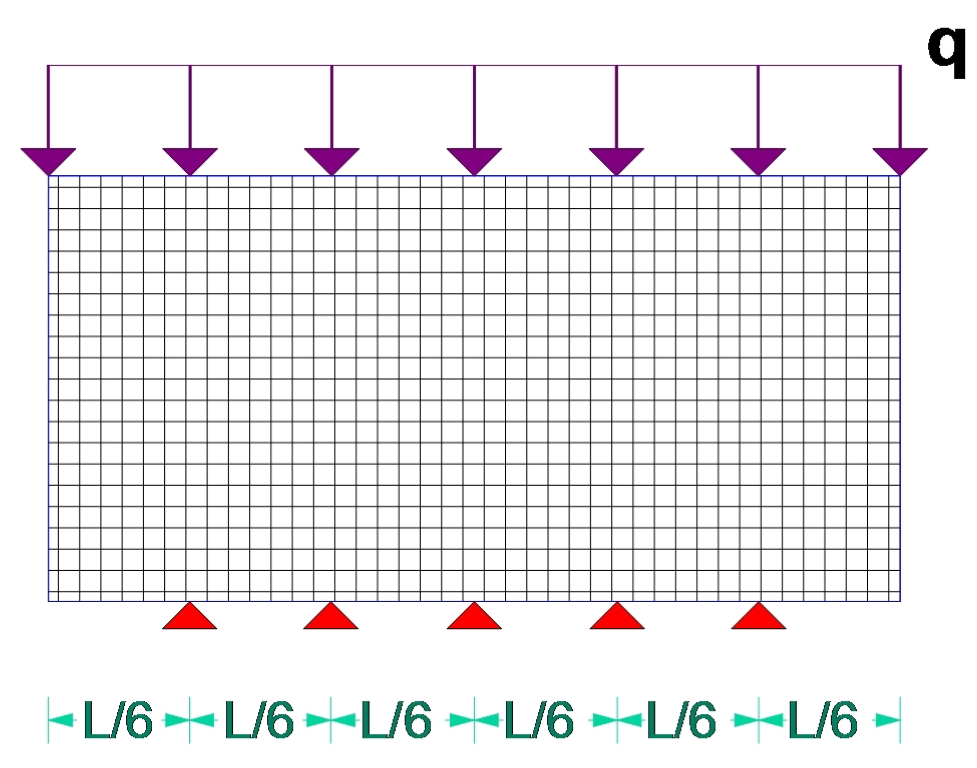
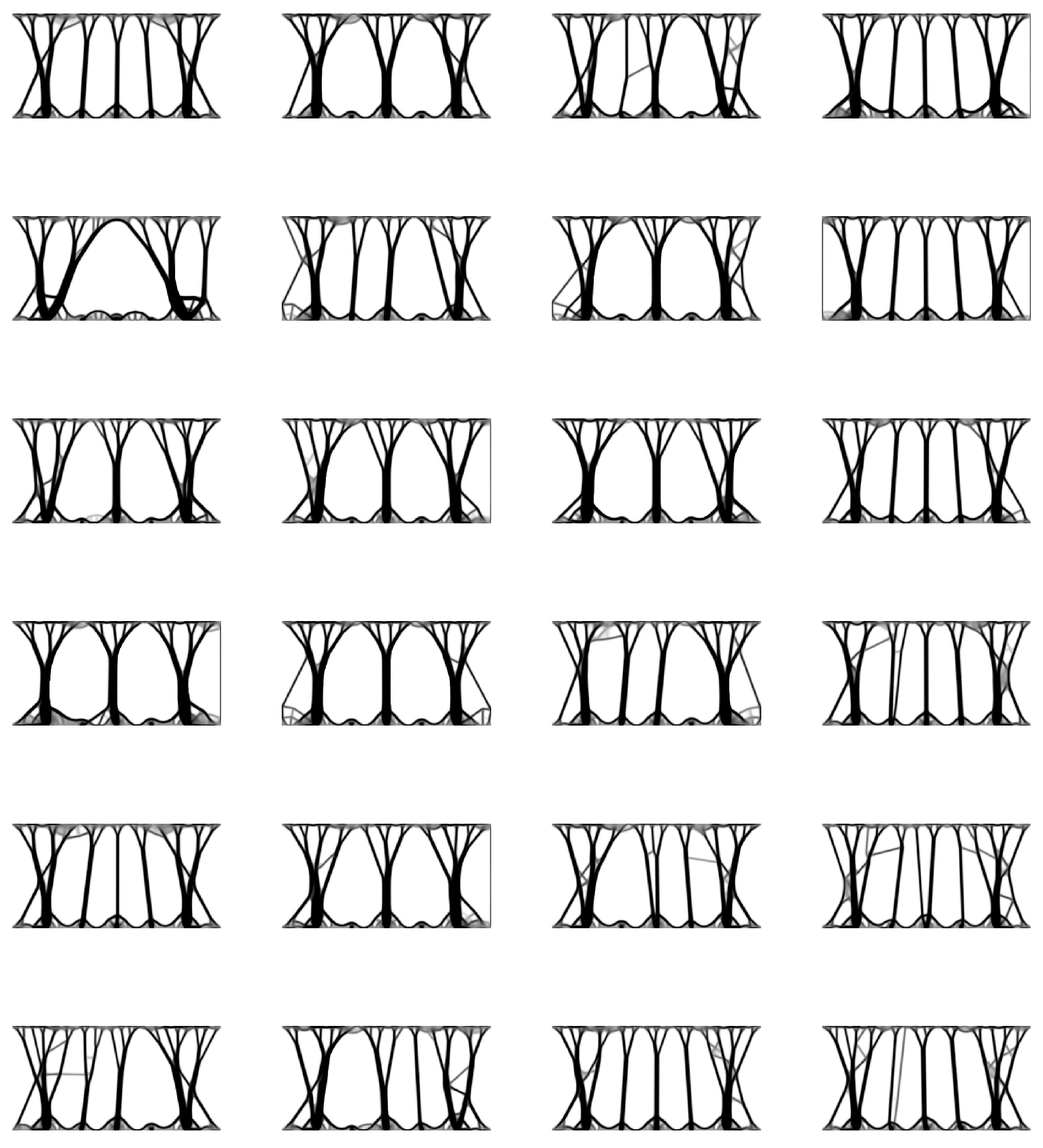
5.3. Test Example C
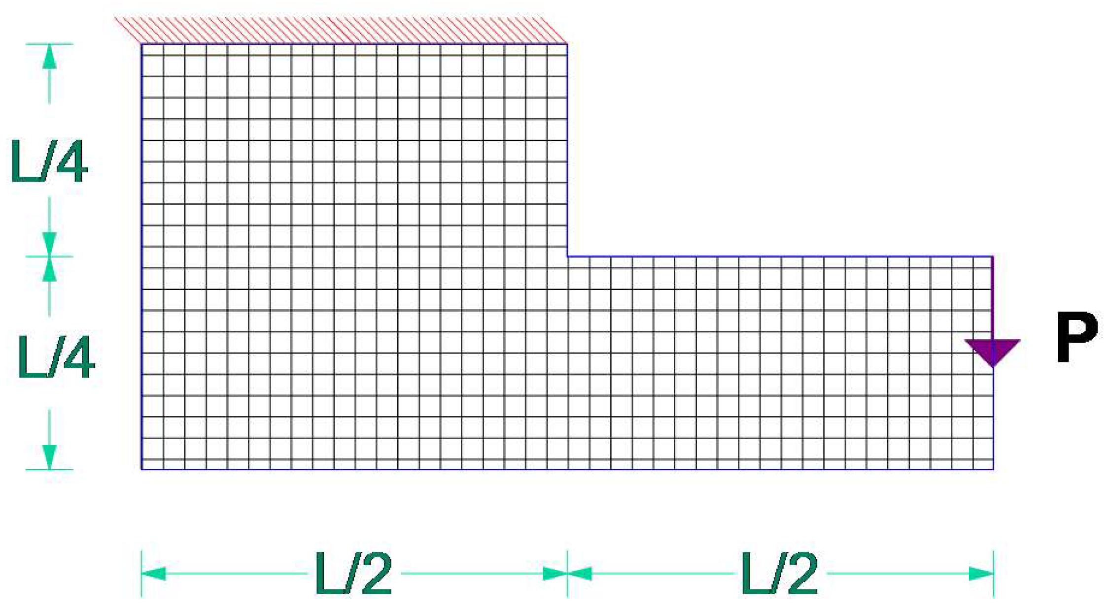
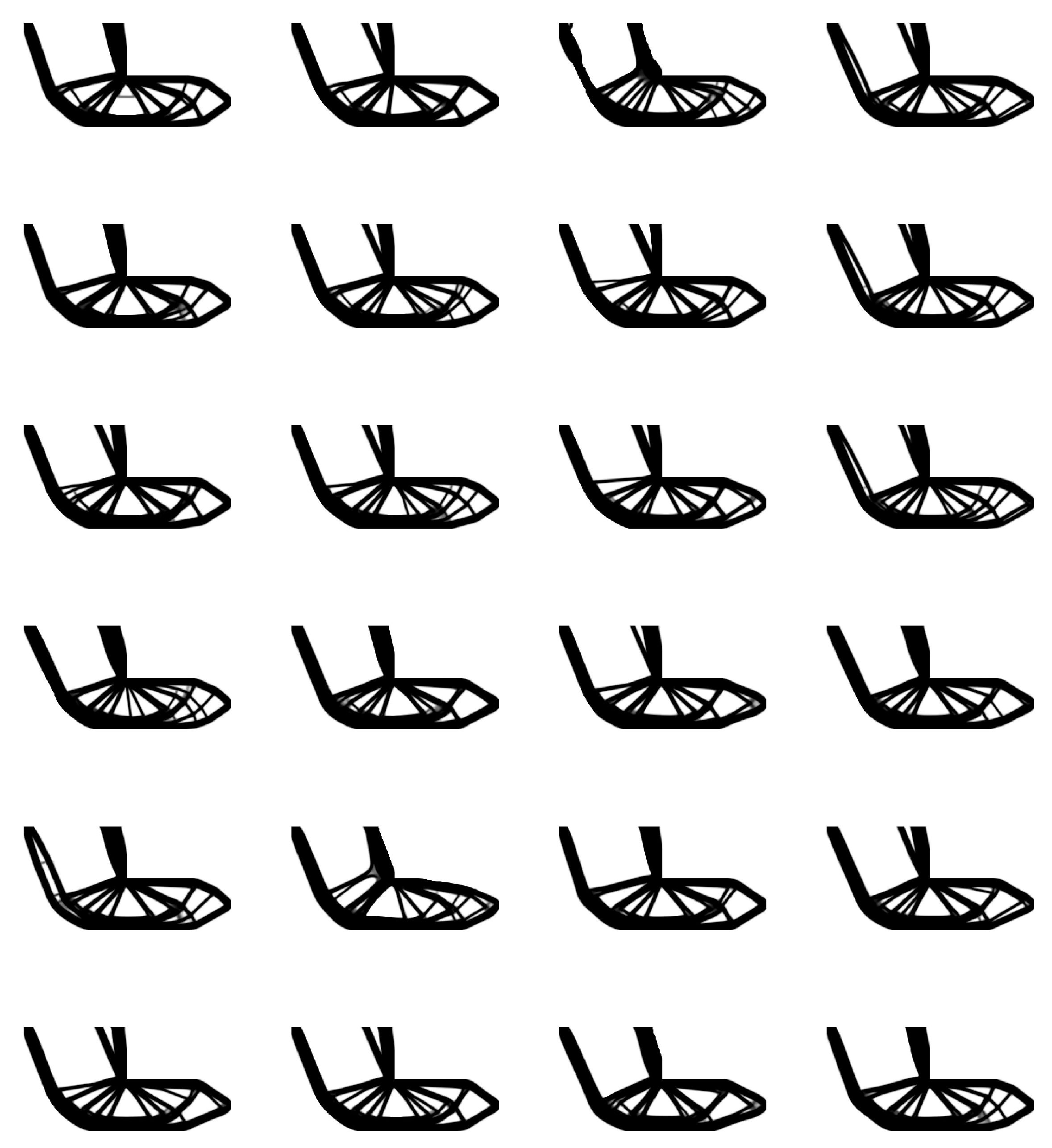
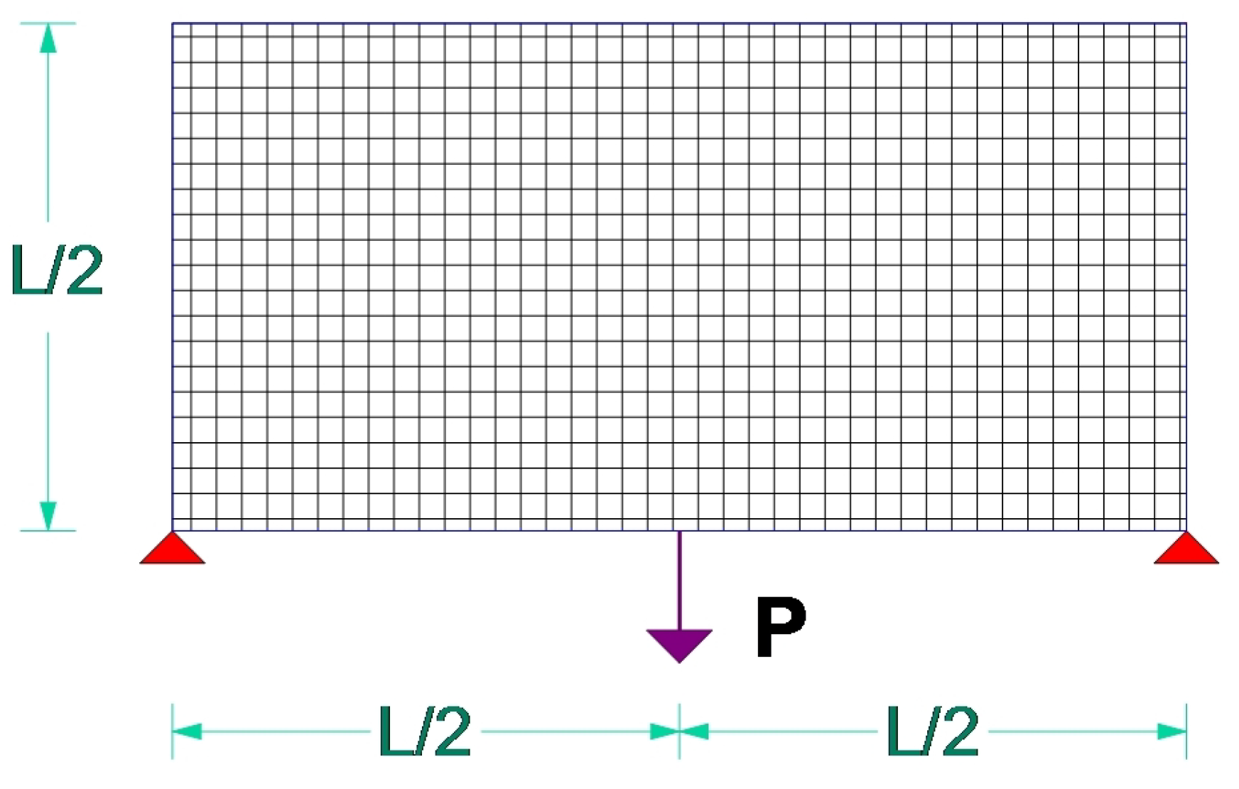
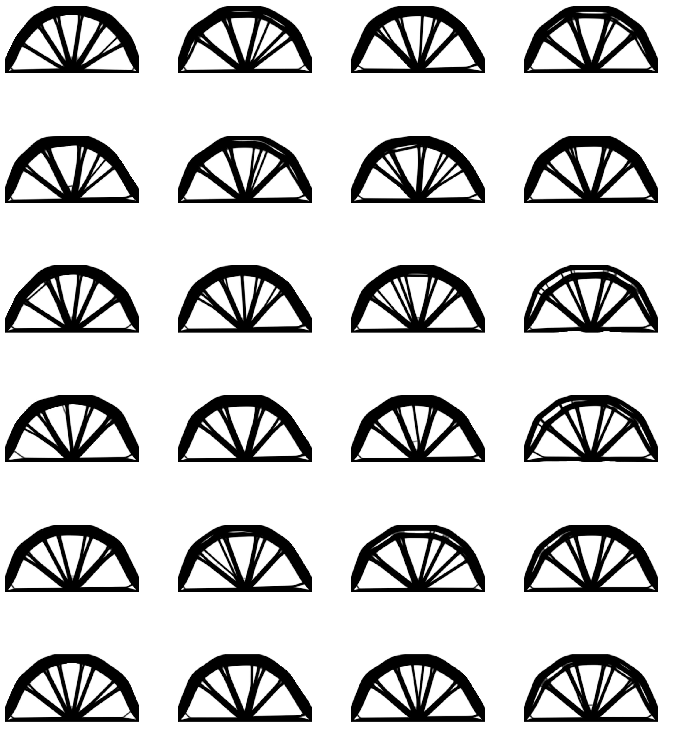
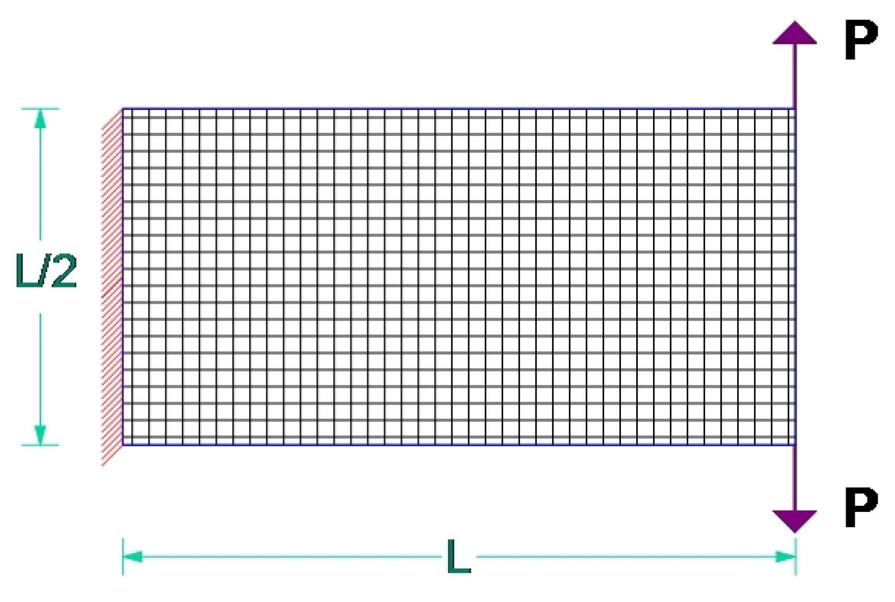
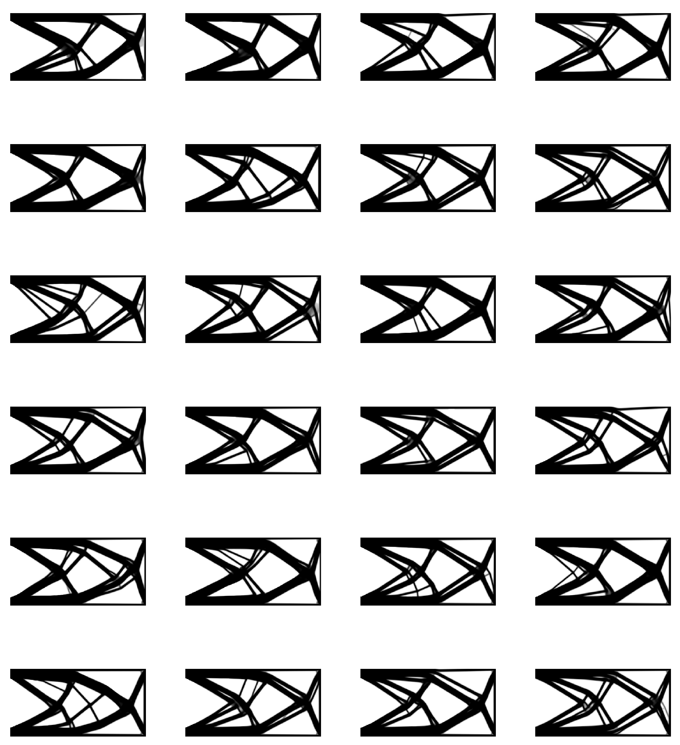
5.4. Test Example D
5.5. Test Example E
6. Discussion
7. Conclusions
Author Contributions
Funding
Institutional Review Board Statement
Informed Consent Statement
Acknowledgments

Conflicts of Interest
Abbreviations
| RNN | Recurrent Neural Networks |
| LSTM | Long Short-Term Memory |
| FE | Finite Element |
| SIMP | Solid Isotropic Material with Penalization |
| STO | Structural Topology Optimization |
| TO | Topology Optimization |
| TOP | Topology Optimization Problem |
References
- Lagaros, N.D.; Papadrakakis, M.; Kokossalakis, G. Structural optimization using evolutionary algorithms. Comput. Struct. 2002, 80, 571–589. [Google Scholar] [CrossRef] [Green Version]
- Lagaros, N.; Plevris, V.; Papadrakakis, M. Multi-objective design optimization using cascade evolutionary computations. Comput. Methods Appl. Mech. Eng. 2005, 194, 3496–3515. [Google Scholar] [CrossRef]
- Kazakis, G.; Kanellopoulos, I.; Sotiropoulos, S.; Lagaros, N.D. Topology optimization aided structural design: Interpretation, computational aspects and 3D printing. Heliyon 2017, 3, e00431. [Google Scholar] [CrossRef]
- Lagaros, N.D.; Vasileiou, N.; Kazakis, G. A C# code for solving 3D topology optimization problems using SAP2000. Optim. Eng. 2018. [Google Scholar] [CrossRef] [Green Version]
- Papadrakakis, M.; Lagaros, N.D. Soft computing methodologies for structural optimization. Appl. Soft Comput. 2003, 3, 283–300. [Google Scholar] [CrossRef] [Green Version]
- Zhang, Z.; Li, Y.; Zhou, W.; Chen, X.; Yao, W.; Zhao, Y. TONR: An exploration for a novel way combining neural network with topology optimization. Comput. Methods Appl. Mech. Eng. 2021, 386, 114083. [Google Scholar] [CrossRef]
- Bendsøe, M.P. Optimal shape design as a material distribution problem. Struct. Optim. 1989, 1, 193–202. [Google Scholar] [CrossRef]
- Zhou, M.; Rozvany, G. The COC algorithm, Part II: Topological, geometrical and generalized shape optimization. Comput. Methods Appl. Mech. Eng. 1991, 89, 309–336. [Google Scholar] [CrossRef]
- Mlejnek, H. Some aspects of the genesis of structures. Struct. Optim. 1992, 5, 64–69. [Google Scholar] [CrossRef]
- Rumelhart, D.E.; Hinton, G.E.; Williams, R.J. Learning Internal Representations by Error Propagation; Technical Report; California Univ San Diego La Jolla Inst for Cognitive Science: La Jolla, CA, USA, 1985. [Google Scholar]
- Fister, I., Jr.; Yang, X.S.; Fister, I.; Brest, J.; Fister, D. A brief review of nature-inspired algorithms for optimization. arXiv 2013, arXiv:1307.4186. [Google Scholar]
- Sigmund, O.; Maute, K. Topology optimization approaches. Struct. Multidiscip. Optim. 2013, 48, 1031–1055. [Google Scholar] [CrossRef]
- Rumelhart, D.E.; Hinton, G.E.; Williams, R.J. Learning representations by back-propagating errors. Nature 1986, 323, 533. [Google Scholar] [CrossRef]
- Schmidhuber, J. Netzwerkarchitekturen, Zielfunktionen und Kettenregel. Ph.D. Thesis, Technische Universität München, München, Germany, 1993. [Google Scholar]
- Kallioras, N. Reduced Order Models and Machine Learning in Analysis and Optimum Design of Structures. Ph.D. Thesis, National Technical University of Athens, Athens, Greece, 2019. [Google Scholar]
- Hochreiter, S.; Schmidhuber, J. Long short-term memory. Neural Comput. 1997, 9, 1735–1780. [Google Scholar] [CrossRef]
- Fischer, T.; Krauss, C. Deep learning with long short-term memory networks for financial market predictions. Eur. J. Oper. Res. 2018, 270, 654–669. [Google Scholar] [CrossRef] [Green Version]
- Tai, K.S.; Socher, R.; Manning, C.D. Improved Semantic Representations From Tree-Structured Long Short-Term Memory Networks. In Proceedings of the 53rd Annual Meeting of the Association for Computational Linguistics and the 7th International Joint Conference on Natural Language Processing (Volume 1: Long Papers); Association for Computational Linguistics: Beijing, China, 2015; pp. 1556–1566. [Google Scholar] [CrossRef] [Green Version]
- Kallioras, N.A.; Kazakis, G.; Lagaros, N.D. Accelerated topology optimization by means of deep learning. Struct. Multidiscip. Optim. 2020, 20, 21–36. [Google Scholar] [CrossRef]
- Dorigo, M.; Stutzle, T. Ant Colony Optimization; The MIT Press: Cambridge, MA, USA, 2004. [Google Scholar]
- Kennedy, J.; Eberhart, R.C. Particle swarm optimization. In Proceedings of the IEEE International Conference on Neural Networks, Perth, WA, Australia, 27 November–1 December 1995; pp. 1942–1948. [Google Scholar]
- Rabanal, P.; Rodríguez, I.; Rubio, F. Using river formation dynamics to design heuristic algorithms. In International Conference on Unconventional Computation; Springer: Berlin/Heidelberg, Germany, 2007; pp. 163–177. [Google Scholar]
- Kallioras, N.A.; Lagaros, N.D.; Avtzis, D.N. Pity beetle algorithm—A new metaheuristic inspired by the behavior of bark beetles. Adv. Eng. Softw. 2018, 121, 147–166. [Google Scholar] [CrossRef]
- Christensen, P.W.; Klarbring, A. An Introduction to Structural Optimization; Springer Science and Business Media: Berlin/Heidelberg, Germany, 2008; Volume 153. [Google Scholar]
- Svanberg, K. The method of moving asymptotes—A new method for structural optimization. Optim. Syst. Theory 1987, 24, 359–373. [Google Scholar] [CrossRef]
- Vogiatzis, P.; Chen, S.; Zhou, C. An Open Source Framework for Integrated Additive Manufacturing and Level-Set-Based Topology Optimization. J. Comput. Inf. Sci. Eng. 2017, 17, 041012. [Google Scholar] [CrossRef]
- Brackett, D.; Ashcroft, I.; Hague, R. Topology optimization for additive manufacturing. In 2011 International Solid Freeform Fabrication Symposium; University of Texas at Austin: Austin, TX, USA, 2011. [Google Scholar]
- Liu, K.; Tovar, A. An efficient 3D topology optimization code written in Matlab. Struct. Multidiscip. Optim. 2014, 50, 1175–1196. [Google Scholar] [CrossRef] [Green Version]
- Allaire, G.; Jouve, F.; Toader, A.M. A level-set method for shape optimization. Comptes Rendus Math. 2002, 334, 1125–1130. [Google Scholar] [CrossRef]
- Querin, O.; Steven, G.; Xie, Y. Evolutionary structural optimisation (ESO) using a bidirectional algorithm. Eng. Comput. 1998, 15, 1031–1048. [Google Scholar] [CrossRef]


| Example | Load Type | Load Num. | Support Type | Support Num. | Volume |
|---|---|---|---|---|---|
| A | Distributed | 1 | Fixed joints | 2 | 40% |
| B | Concentrated | 1 | Fully fixed | 1 | 35% |
| C | Distributed | 1 | Fixed joints | 5 | 25% |
| D | Concentrated | 1 | Fixed joints | 2 | 45% |
| E | Concentrated | 2 | Fully fixed | 1 | 50% |
Publisher’s Note: MDPI stays neutral with regard to jurisdictional claims in published maps and institutional affiliations. |
© 2021 by the authors. Licensee MDPI, Basel, Switzerland. This article is an open access article distributed under the terms and conditions of the Creative Commons Attribution (CC BY) license (https://creativecommons.org/licenses/by/4.0/).
Share and Cite
Kallioras, N.A.; Lagaros, N.D. MLGen: Generative Design Framework Based on Machine Learning and Topology Optimization. Appl. Sci. 2021, 11, 12044. https://doi.org/10.3390/app112412044
Kallioras NA, Lagaros ND. MLGen: Generative Design Framework Based on Machine Learning and Topology Optimization. Applied Sciences. 2021; 11(24):12044. https://doi.org/10.3390/app112412044
Chicago/Turabian StyleKallioras, Nikos Ath., and Nikos D. Lagaros. 2021. "MLGen: Generative Design Framework Based on Machine Learning and Topology Optimization" Applied Sciences 11, no. 24: 12044. https://doi.org/10.3390/app112412044