1. Introduction
Structural integrity (diagnosis) analysis and estimation of useful life (prognosis) is carried out with the help of an array of sensors in a Structural Health Monitoring (SHM) system [
1]. However, reliable diagnosis and prognosis of the health of a structural system based on input–output measurements are complicated and actively pursued by researchers around the world. With the advancement of smart materials, the focus is mainly on real-time structural monitoring, which can be evolved into condition-based maintenance philosophies [
2]. Earlier work on damage identification and health monitoring of structural and mechanical systems, from changes in dynamic characteristics to the response of structures, can be found in an extensive literature survey by Doebling et al. [
3]. An ideal structural damage detection system is capable of detecting small structural damages at an early stage, locating the damaged members and estimating the extent of the damage so that the remaining life of the structure can be estimated or mitigating measures can be undertaken. Structural damages, if not detected in time, will lead to progressive damage and will adversely affect the structural integrity. Failure to detect damages earlier also leads to increased cost of repairs. In a recent review of the structural monitoring programs implemented in the United States, Nagarajaiah and Kalil [
4] have highlighted the importance of an SHM program as a powerful tool for structural damage and condition assessment of large-scale civil infrastructures after potentially damaging events.
A vibration-based SHM system contains useful information about the dynamic characteristics of a system for structural damage detection. Vibration-based structural damage detection methods are categorized into frequency domain methods and time domain methods. Frequency domain methods are mainly considered as offline methods since signals from the time domain method are processed to obtain modal information in the frequency domain. Comparison of modal information with the healthy system gives an indication of structural damage [
5]. The sensitivity of the modal characteristics to the structural damages makes it difficult to identify small structural changes. All frequency domain methods are modal-based methods, and a reliable analytical model is necessary for the successful application of frequency domain methods. Moughty and Casas [
6] have drawn attention to the fact that modal-based damage detection techniques find limited real-world applications due to shortcomings stemming from environmental and operational variations and overreliance on modal-based Damage Sensitive Features (DSFs). Using measured input–output data from the vibration of a structure, entries in the system matrices are modified to reproduce the measured data [
7]. Modal parameters of the damaged structure are compared with the modal parameters obtained from the analytical model of the structure, and error is minimized by iteratively refining the stiffness and mass matrices. Perturbation in mass matrices and stiffness matrices gives spatial information about damage, while quantitative analysis of the perturbation matrix can help in estimating the severity of the damage. Kauok [
8] used the minimization of the rank of perturbation matrix to update the optimal matrix instead of using minimization of the norm of the perturbation matrix [
9,
10]. Park [
11] has emphasized the importance of continuous vibration monitoring together with statistical feature extraction algorithms for their application to structural health monitoring.
Finite element model updating methods is one of the efficient, non-destructive and global identification techniques used. However, the main challenge for large structures that are tested in operational conditions is to identify enough modal parameters with sufficient accuracy [
12]. Reynders et al. [
12] have proposed operational modal analysis with the exogeneous inputs (OMAX) approach, where an artificial force is used in operational conditions and a structural model is identified that takes both the forced and the ambient excitation into account. Teughels and Roeck [
13] used experimental eigenfrequencies and mode shapes to tune the stiffness properties of the elements in the FE model update. Zhan et al. [
14] have used a grillage method to create the adjacent precast PC box beam bridge models and used minimization of coherence function of response spectrum (CFRS) indices in the model updating method. The response spectra of two adjacent beams obtained by applying fast Fourier Transform (FFT) of either velocity or acceleration response vectors from the coupled vehicle-bridge vibration analysis model are used for CFRS index calculations. Zhou and Tang [
15] have formulated a multi-response Gaussian process (MRGP) meta-modeling approach to inversely identify model parameters through sampling in the FE model updating methodology.
The response of the damaged system is different from that of the healthy system and forms the basis of the time domain methods. Structural damage detection filters are designed to detect structural damage in real-time by observing the residuals from each filter. Earlier work is attributed to failure detection, where the aim was to detect failure among sensors, actuators, and structural members and to make the failure detection algorithm robust with respect to system uncertainties and noise corrupted measurements [
16]. In the course of development, fault detection based on analytical redundancy has emerged. Analytical Redundancy (AR) is based on the mathematical model of the system, where the inherent redundancy contained in the static and dynamic input–output is exploited. However, input–output measurements are coupled, and the structural changes at one location results in changes in output measurements at several locations. Phan et al. [
17] provided an interaction matrix formulation to decouple output error signals. Koh et al. [
18] detected and tracked failure among the actuators in real-time via decoupling of input–output measurements. Beard [
19] and Jones [
20] were among the first ones to implement modal-based observers as failure detection filters in the early 1970s. The second-order version of Beard’s failure detection filter was developed by Kranock [
21] and an applied filter-based approach to identify structural damage as well as the location of damage in real-time. Seibold et al. [
22] used the Kalman filter bank approach for the damage detection method in the rotor dynamic system. In another study, Seibold [
23] applied the extended Kalman filter with a recursive instrumental variables technique to estimate the crack development in a rotor with measured displacement in the disc. Dharap et al. [
24] applied ARMarkov observers to estimate the severity of the damage in a planar truss structure. However, depending upon the accuracy with which structural damage needs to be estimated, a large number of ARMarkov observers are necessary for its successful application to structural health monitoring. Due to the unique input error function for each individual structural member, the proposed algorithm in this study overcomes the limitation of a large number of ARMarkov observers, system uncertainties, and noisy output measurements. Either deterministic methods or probabilistic methods are implemented to address system uncertainties. Ideally, a single set of optimal parameters that accurately represent the structural system are targeted. However, due to the complexity of the structural system with intertwined input–output measurements, probabilistic methods are preferred. Model updating based on Baysian inference is commonly used for SHM applications. Sun and Betti [
25] implemented a hybrid optimization methodology formulated within a Baysian inference framework for model updating of a LANL three-story frame structure in the presence of measurement noise and system uncertainties. In another study, Sun et al. [
26] used intrinsic building impulse response functions (IRFs) from ambient excitations and proposed a hierarchical Baysian framework with Laplace priors for updating the FE model. Zhou and Tang [
27] adopted a Markov chain Monte Carlo (MCMC) procedure for Baysian inference-based model updating. It is still challenging to apply a Bayesian inference approach to a large-scale complex system. The algorithm proposed here is based on the interaction matrix formulation resulting in input error functions where decoupling of input-output measurements is accomplished. Since one-to-one correlation is established between an error function signal and a structural member, a simple error minimization function can be implemented.
Since the discovery in early 1990 by Iijima [
28], carbon nanotubes (CNT) have been widely pursued as nanofillers for nanocomposites due to their high aspect ratios and stronger mechanical, electrical and thermal properties [
29]. Very high values of dielectric permittivity and electric conductivity are observed near a percolation threshold; a critical concentration of CNTs is extremely sensitive to external parameters such as temperature, pressure and deformations [
30,
31]. Carbon nanotube composites find a wide range of applications and have been actively pursued as a smart structural material, which can be used as a sensor to monitor stiffness degradation as the structure is subjected to external loads. Alexipoulous et al. [
32] examined applications of glass fiber-reinforced polymer (GFRP) coupons with embedded CNTs as sensors. In another study, Al-Rub et al. [
33] explored multi-walled CNTs as reinforcement in cementitious materials. Loh and Nagarajaiah [
34] present a comprehensive review of the application of carbon nanotube composites as sensors for structural health monitoring applications. The proposed methodology in this paper is envisioned for its application to real-time structural health monitoring of smart structures composed of CNT embedded polymers such as structural material as well as wireless, self-sensing CNT sensors.
The majority of SHM techniques are developed on conventional instrumentations, such as linear variable differential transducers (LVDT), accelerometers or strain gauges attached to the structure, but recent developments involve more novel non-contact techniques such as acoustic emission (AE)-based or vision-based. Rabiei and Modarres [
35] have studied in situ AE measurements from notched aluminum specimens to detect and track the propagation of the crack under cyclic loading and proposed quantitative methods using AE measurements for quantitative Structural Health Monitoring (SHM). Piezoelectric transducers have an advantage over the conventional strain gauges due to high bandwidth, mostly linear properties and easy embedment to the structure and are widely adopted as sensors and actuators. In addition to finding applications for vibration-based approaches and wave propagation base approaches, piezoelectric transducers are also explored for impedance/admittance-based methods. Shuai et al. [
36] have devised an impedance/admittance-based pre-screening scheme by implementing piezoelectric transducers to rank the likelihoods of fault locations with estimated severity levels. Yapar et al. [
37] have implemented piezoelectric receivers as AE sensors during experimental setups of model bridge girders composed of reinforced concrete beams, prestressed concrete beams and steel beams. Giurgiutiu et al. [
38] have explored piezoelectric wafer active sensors using an electro-mechanical (E/M) impedance method for near field damage detection and wave propagation methods for far-field damage detection on realistic aging aircraft panels with seeded cracks and corrosion.
Withey et al. [
39] have applied Single-Walled Carbon Nanotube Composite Coatings to a test specimen and measured spectral shifts of the nanotube near-infrared fluorescence peaks using a circularized-beam diode laser. As the technology is improving, video cameras with higher frame rates and resolutions are becoming available at a reduced cost and finding their application in structural health monitoring. Feng and Feng [
40] have identified natural frequencies and mode shapes of a simple supported beam structure from measurements using one video camera and show good correlation between the data obtained using an array of accelerometers. In another study, the authors of [
41] have evaluated the performance of the proposed vision sensor for dynamic displacement measurements via shaking table experiments on a scaled three-story frame structure and those measured by high-performance laser displacement sensors. Chen et al. [
42] have identified vibration frequencies and mode shapes of the World War I Memorial Bridge in Portsmouth by measuring displacements with a developed video processing technique.
Deep learning technologies can be implemented for vibration-based structural monitoring, but it is essential to have algorithms that can correlate the measured signal to the present status of the structure [
43]. The current study is an attempt to provide one of such algorithms for real-time structural health monitoring and condition-based maintenance. Using the proposed algorithm, the stiffness of individual structural members can be estimated, and an updated analytical model can be made available for further evaluation. A unique error function corresponding to individual structural members is established using an interaction matrix formulation and enables implementing optimization techniques by minimizing the input error function signal. The entire process can be automated for real-time stiffness tracking of structural members, and the proposed algorithm manages system uncertainties very well. The statistical approach is easy to implement in order to address uncertainties in estimating structural stiffness from noise in input–output measurements. This paper is organized as follows. We will present the input error function formulation in
Section 2. Observers based on the input error function are discussed in
Section 3 to track the stiffness variation in all three springs for a three spring-mass-damper system. Optimization of the input error function is discussed in
Section 4 where the robustness of the proposed input error functions for estimating the severity of damage in structural members is verified. Finally, the proposed optimization of the input error function technique is used to track stiffness variation in the structural member for a three-bay two-dimensional truss structure (as in long span bridge trusses) in
Section 5.
2. Theoretical Background
In this section, the mathematical formulation for the equivalence of stiffness change and actuator failure is derived. The second-order dynamic system in physical coordinate
, with the external input
is denoted as
,
and
represent the mass, damping and stiffness matrices, respectively. The input influence matrix
associates each input to the corresponding degree of freedom. The structural changes to an individual structural member updates the corresponding entries in the global stiffness matrix. When compared to global undamaged stiffness matrix
, changes due to structural changes in stiffness of the members can be expressed as
Any structural updates resulting in changes in stiffness of the members are captured by the term
. Structural damage results in decreasing stiffness, while structural strengthening results in increasing the stiffness of the member. The term
can be viewed as input error
, and Equation (2) can be rewritten as
Since each output is influenced by all other inputs, it is not obvious to identify the location of structural damage. An actuator failure detection algorithm [
13,
14] presents a formulation that can decouple the influence of one actuator on the output measurements. Previously, actuator failure formulation was implemented by Koh et al. [
29] using an analogy between stiffness change and input error for structural damage detection and localization. Stiffness variation in individual spring elements for a three DOF spring-mass-damper system is identified in real-time; however, no attempt is made to estimate the severity of damage.
For the sake of completeness and ease of reference, only critical steps for the input error function formulation [
44] are included here. The development of the input error function is in a state-space framework, and hence, Equation (1) is rewritten in first-order form. Assuming an
-th order,
-input,
-output discrete-time model of a system in state-space format
The special interaction matrix formulation is introduced below, which will be a key in establishing a connection between state space models and input–output models [
17]. Substituting repeatedly for some
, Equation (4) takes the following form
starting with
and
and going
steps into the future, column vectors of output data
and input data
are obtained
Controllability matrix
of the order of
, an observability matrix,
of the order of
and the “Toeplitz” matrix of the system of Markov parameters
of the order of
from Equation (5) can be written in terms of state space formulation, as shown in Equation (7)
Considering the contribution of each individual input
, Equation (5) can be rewritten as
where
The
matrix becomes a null matrix if the measurements are displacements. Acceleration measurements can be easily accommodated with a simple modification [
17]. With the introduction of an interaction matrix
, Equation (8) can be written as
Interaction matrix
enables decoupling the influence of changes to the stiffness of the members in output measurements except, for the term
. Pre-multiplying the Equation (10) by
results in
The number of independent sensors needs to be at least equal to the number of structural members (
) to ensure the existence of
such that failure among each structural member can be distinguished. This also ensures an orthogonal row vector
to all remaining column vectors
Introduction of an orthogonal row vector
has eliminated the influence of the term
in Equation (11), provided conditions in Equation (12) are satisfied. Equation (11) thus can be written in terms of each input
, by pre multiplying by a vector
Using Equation (13), input error function can be written in general form by accounting for actuator error
such that
using coefficients
and
. Introduction of coefficients
and
are critical in transforming Equation (14) to a scalar equation. A unique relationship is established between an error function and a particular structural member. This is a key to uncoupling the influence of structural members on all output measurements except one and enables tracking the stiffness variation in structural members using the input error function in Equation (13).
Coefficients
(are
row vectors) and
(scalars) in Equation [
14] above are related to the terms in state space formulation as indicated in Equation (15) below
3. Three DOF Mass-Spring-Damper System
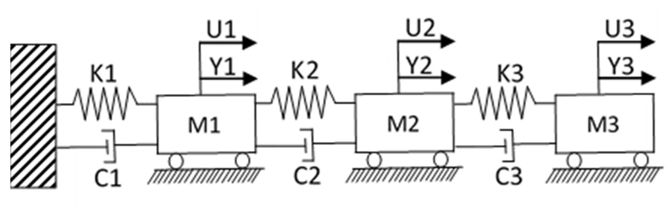
Three Degree of Freedom (DOF) spring-mass system, as shown in
Figure 1, is considered to illustrate the proposed stiffness tracking algorithm. Stiffness change
is replaced by internal input forces
to the DOFs, where the structural member is connected. Thus, stiffness change in spring K2 will result in additional input forces at DOF 1 and 2 and stiffness change in spring K3 will result in additional input forces at DOF 2 and 3. Since the other end of spring K1 is fixed, the stiffness variation in spring K1 will result in additional input force at DOF 1 only. Initial stiffness of each spring is assumed to be 100 N/m, and mass at each node is assumed to be 1 Kg. Proportional damping is considered, though non-proportional damping can be considered without loss of generality. To monitor the stiffness change in all three springs, the system has three inputs (
) and three output sensors (
) at nodes 1, 2 and 3.
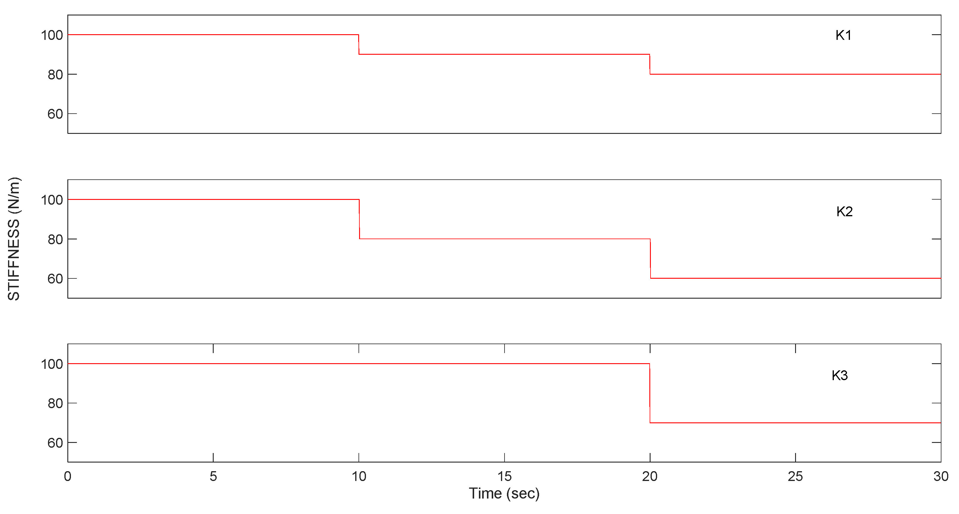
Figure 2 plots the stiffness variation in individual springs used for simulating input–output data. As it can be observed, initially up to 10 s, a spring-mass damper system is considered to be healthy. Stiffness degradation in an individual spring is considered after 10 s. The stiffness of spring K1 is assumed to be 90 N/m between 10 and 20 s and 80 N/m after 20 s, whereas the stiffness of spring K2 is assumed to be 80 N/m between 10 and 20 s and 60 N/m after 20 s. Spring K3 is assumed to be undamaged till 20 s, and stiffness of 70 N/m is assumed after 20 s. A series of input error function observers is designed for each spring. The number of observers will depend upon the accuracy of the stiffness estimation.
Figure 3 plots the data from the input error function observers. Non-zero error is an indication of mismatch between assumed stiffness and actual stiffness of spring, whereas zero error indicates the correct observer and corresponding stiffness of the spring is the estimated correct stiffness of the spring. For brevity, observers for all three springs are included in
Figure 3 in increments of 10 N/m beyond the stiffness value of 60 N/m only. Zero input error for a stiffness value of 100 N/m till 10 s is observed for spring K1. Zero input error for a stiffness value of 90 N/m for spring K1 is observed between 10 and 20 s, and finally, zero input error for a stiffness value of 80 N/m for spring K1 is observed beyond 20 s. Thus, it can be concluded that spring K1 is undamaged till 10 s and has a stiffness of 90 N/m between 10 and 20 s and stiffness of 80 N/m beyond 20 s. Zero input error correctly follows the stiffness change shown in
Figure 2 for spring K1. Similarly, it can be concluded that spring 2 is undamaged till 10 s and has a stiffness of 80 N/m between 10 and 20 s and stiffness of 60 N/m beyond 20 s. Spring K3 is undamaged till 20 s and has a stiffness of 70 N/m beyond 20 s. Input error function observers have decoupled the influence of each individual spring on the output measurements and are able to track the stiffness variation in all three springs in real-time.
Stiffness variation in individual springs, as shown in
Figure 2, is arbitrarily chosen to underline the robustness of the proposed methodology using a set of observers. For brevity, only a limited number of observers are included in
Figure 3. Since the stiffness variation considered is of the order of 10 N/m, observers presented in
Figure 3 are in increments of 10 n/m. Without loss of generality, any stiffness variations in individual springs can be considered. The number of observers per structural member should be determined on the level of accuracy with which stiffness variation needs to be tracked and the level of accuracy that can be achieved for practical applications. The presence of unwanted noise in input–output measurements will affect the accuracy of the tracked stiffness estimations.
Thus, it can be concluded that input error function observers can track stiffness variation in individual structural members. As a result, reliable analytical models of the structure can be made available by implementing input error function observers rather than relying on the accuracy of the analytical model. It can be observed that proposed input error function observers overcome the limitation of a large bank of ARMarkov observers [
20]. Successful implementation of the ARMarkov observer approach for estimating the severity of damage must account for all the combinations of the stiffness variation in individual structural members. This will result in a very large bank of ARMarkov observers and makes it less attractive for real-world applications to track stiffness variation in multiple members. Since the input error function is independent of the stiffness of other structural members, only a limited number of observers for each structural member are needed to track the stiffness variation. Since the observer-based approach requires a manual decision based on the input error functions as presented in
Figure 3, it would still be a challenge to implement for online structural health monitoring. To automate the updating of stiffness of structural members, an optimization of the input error function is proposed in the next section.
4. Optimization of Input Error Function Three DOF Mass-Spring-Damper System
Instead of using a bank of input error observers for estimating change in stiffness, input error minimization of a damaged structural member is proposed for tracking the stiffness variation of a structural system in real-time.
Figure 4 below shows the workflow of the entire process. Using the input error function formulation, the error signal for each structural member is established. The interaction matrix
formulation and introduction of vector
has completely decoupled the influence of stiffness variation in individual structural members on the output measurements. This enables tracking the stiffness variation in each structural member by using the error function formulation in Equation (14). As indicated in
Figure 3, a zero-error signal is obtained when the correct stiffness estimation is used. The stiffness estimation process to obtain a zero-error signal is automated by implementing an optimization technique. The optimization parameter (stiffness value) corresponding to the optimized zero-error signal will be indicative of the stiffness of the structural member under consideration. Otherwise, for the intertwined influence of stiffness variations on output measurements, using an interaction matrix formulation, a one-to-one correlation is established between an error function and an individual structural member. This unique relationship between the structural members, as represented by blocks “Member N” and an error signal block “EN” in
Figure 4, makes it possible to optimize the error signal, which is a function of the stiffness of a structural member. Thus, the structural stiffness of each individual member can be obtained to establish an accurate analytical model of the system.
Input–output measurements are generally corrupted with unwanted, random signals, referred to as noise. The presence of noise in the input–output measurements affect the system identification results. Even a small percentage of noise affects the estimation of the stiffness matrix. To study the effect of noise, output measurements are corrupted with 2%, 5% and 10% rms white noise for the three DOF spring-mass-damper system. It is assumed that noise at output measurements is a random phenomenon and there is no correlation between different output measurements. Unbiased randomness of the noise in output measurements can be addressed by applying an averaging scheme, which should cancel out the effects of noise in estimating the stiffness of individual springs. Monte-Carlo simulations for the input–output measurements are carried out, and using 100 different random input–output measurements, the stiffness of each spring is estimated.
Figure 5 plots the variation in estimation of stiffness in springs K1, K2 and K3 for different % rms white noise in output measurements. The data bars in “red” indicate the correct stiffness of the corresponding spring used in numerical simulations, and the data bars in “blue” indicate the estimated stiffness with optimization of an input error function. It should be noted that data presented in “blue” are the estimated stiffness values in the range as indicated along the
x-axis and the number of estimations normalized with the total number of Monte-Carlo simulations as indicated along the
y-axis. As the % rms noise is increased from 2% to 10%, more scatter in the estimation of stiffness can be observed.
Table 1 summarizes the data for 100 iterations. It can be observed that even in the presence of 10% rms noise, stiffness estimation for individual springs is remarkably close to the actual stiffness. Although stiffness estimation is close to the actual stiffness, an increase in % rms noise results in an increase in scatter, as evident from plots in
Figure 5 and the standard deviation listed in
Table 1. A greater standard deviation indicates less confidence in the estimation of stiffness and vice versa.
Robustness of the proposed optimization process for stiffness estimation verifies the potential for implementing input error function for real-time structural health monitoring where stiffness variation in individual structural members can be tracked in real-time. Monte-Carlo simulations result in an input error function optimization methodology that is very robust with respect to % rms noise. However, it is difficult to carry out Monte-Carlo simulations in practice. Obtaining different input–output combinations is a time-consuming process and thus not practical. Hence, an optimization procedure needs to be developed when only limited input–output measurements are available. One such solution is considered here where random white noise is given as an input to the system and output is measured at all DOFs. Imposing this condition on the interaction matrix , such that , makes the system independent after steps. By shifting the window , uncorrelated input–output measurement sets are obtained. These uncorrelated input–output measurements can be used as a substitute for the Monte-Carlo simulations, and an averaging strategy can be implemented by shifting the data points used for optimization of the input error function.
In this simulation, stiffness of the spring K1 is assumed to be 80 N/m, K2 is assumed to be 60 N/m and K3 is assumed to 75 N/m. For brevity only, the histograms with different data points to estimate the stiffness of spring K2 are plotted in
Figure 6. The presence of noise is simulated with consideration of 5% rms white noise in the output measurements. Different lengths of the data are used for optimization of the input error function for spring K2. When only 200 data points are used, it results in a large spread in the data for the estimation of stiffness for spring K2. As the number of data points are increased to 800, spread in the data is reduced.
Table 2 summarizes the data for all three springs. Consistent with the trend shown in
Figure 6 below, it can be observed that for all three springs, as the number of data points is increased from 200 to 800, spread in the stiffness estimation is reduced, indicated by greater standard deviation values corresponding to 200 data points and lesser standard deviation values corresponding to 800 data points.
Table 2 summarizes the statistics of the input error function for the individual springs K1, K2 and K3. Trends as discussed about the Spring K2 can also be observed for Spring K1 and Spring K3 as the number of data points are increased from 200 to 800. The mean values of the stiffness estimation for individual springs are close to the actual values used in simulation with increasing confidence in the estimation as the number of data points used in the estimation are increased.
5. Numerical Simulation for Stiffness Tracking: Two-Dimensional Three-Bay Truss Structure
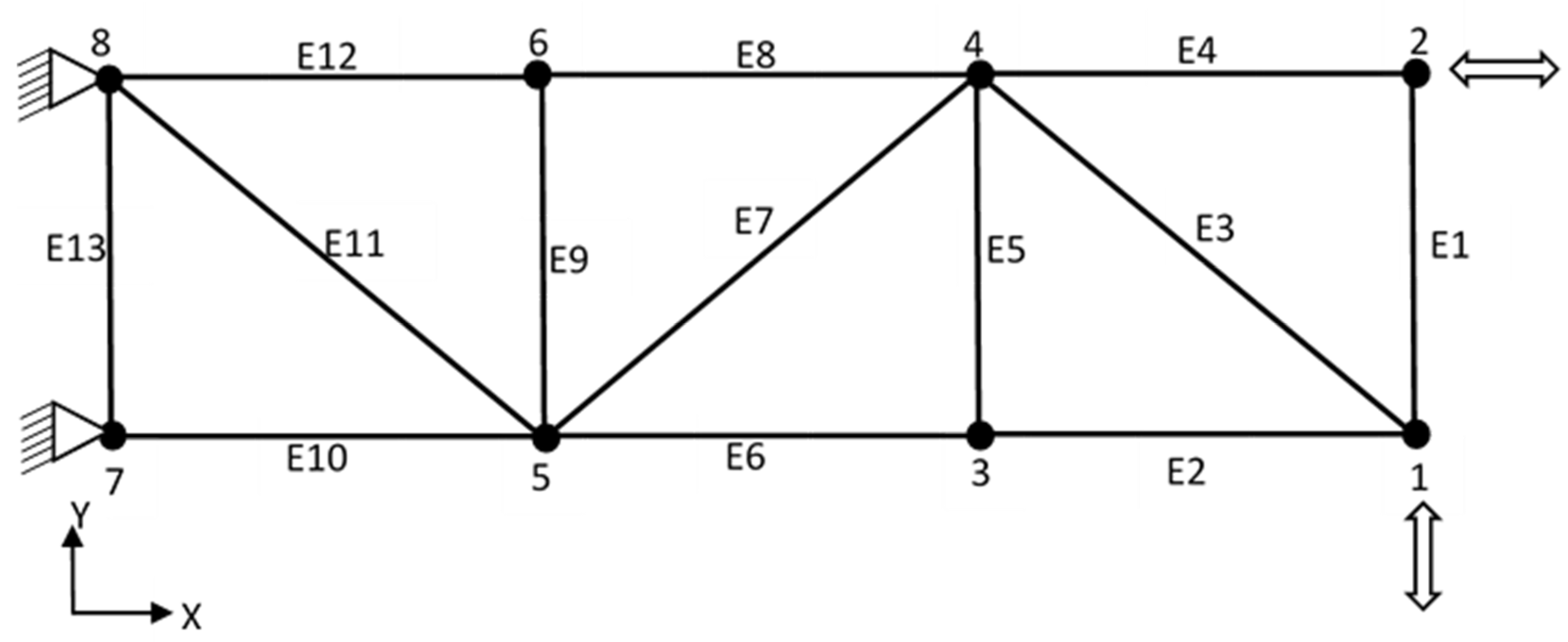
An analytical model of the two-dimensional three-bay truss structure representing a bridge structure is considered here to validate the proposed methodology of optimization of the input error function for stiffness tracking in structural members. Details of the planar truss structure are shown in
Figure 7. Excitation is provided to the planar truss with two inputs at the nodes 1 (Y-direction) and 2 (X-direction), as shown in
Figure 7.
Figure 8 plots the stiffness degradation in a truss member # E10 assumed during numerical simulations. As shown in
Figure 8, truss member # E10 is assumed healthy till 500 s and has a stiffness degradation of 20% between 500 and 1000 s. Structural degradation continues and truss member # E10 loses another 10% of stiffness between 1000 and 1500 s and a further 10% resulting in total degradation of 40% between 1500 and 2000 s.
Optimization of the input error function is implemented to track the stiffness variation in truss member # E10. To simulate practical applications, a sensitivity study for the % rms noise is carried out. Noise of 2% rms, 5% rms and 10% rms is added to the output measurements.
Figure 9 plots the stiffness variation as tracked by optimization of an input error function corresponding to truss member # E10. For comparison purposes, stiffness ratio estimations for an ideal system without any noise are also included in
Figure 9. Significant spikes with reference to the idea scenario is evident for data corresponding to 5% rms and 10% rms noise in output measurements. However, the mean values reported in
Table 3 clearly show the robustness of the proposed method. Stiffness estimation is within 2% even for 10% rms noise, though bigger spikes give less confidence in the stiffness estimations.
A sensitivity study for the number of data points used for estimation of stiffness in truss member # E10 is also carried out, and stiffness tracking is plotted in
Figure 10. Please note that only 5% rms noise is considered here. Relatively bigger spikes can be observed for stiffness ratio estimation values corresponding to 200 data points, whereas stiffness ratio estimations corresponding to 800 data points closely follows the actual stiffness ratio. However, stiffness ratio estimations listed in
Table 4 show an accurate stiffness ratio estimation for any number of data points used. The mean value of the stiffness estimation in
Table 4 is less sensitive to the number of data points used when compared to the sensitivity of the stiffness estimation data for % rms noise considered in
Table 3.
For brevity, the stiffness variation of only one member, #E10, is tracked here. This member will be a representative of a member critical to the structural integrity of the system under consideration. Without loss of generality, the stiffness variation in any of the truss members can be tracked using the proposed algorithm in this study. However, the proposed algorithm will have limitations inherent to the structural system under consideration. Changes in output measurements will not have the same level of sensitivity to the changes in stiffness of all the structural members and will be a function of load path and location of input–output measurements. The proposed methodology has the limitation that the number of independent sensors needs to be at least equal to the number of structural members so that failure among each structural member can be tracked.
For practical applications, implementing Monte Carlo simulations will result in expensive computational costs and might delay the decision process to support real-time tracking depending upon the complexity of the structural system under monitoring. If necessary, computational burden can be addressed by tracking only members critical to the structural integrity. A structural health monitoring system can be envisioned where an alarm can be triggered once a certain threshold is crossed for critical members, and from then onwards, the whole structural system will be closely monitored. In this study, analytical redundancy because of structural stiffness changes is considered in this study. The influence of other factors such as variations in the mass, damping values or environmental factors that will result in a different system response when compared to the assumed theoretical system are beyond the scope of this paper. However, if the effect of such factors is local and will result in stiffness change locally, the algorithm proposed in this paper will be able to identify the stiffness variation, but further work is needed to make a distinction between structural stiffness changes and other changes such as variations in mass, temperature or damping values.


