Dynamic Damage Mechanism and Seismic Fragility Analysis of an Aqueduct Structure

Abstract

The Concrete Damaged Plasticity (CDP) constitutive is introduced to study the dynamic failure mechanism and the law of damage development to the aqueduct structure during the seismic duration using a large-scale aqueduct structure from the South-to-North Water Division Project (SNWDP) as a research object. Incremental dynamic analysis (IDA) and multiple stripe analysis (MSA) seismic fragility methods are introduced. The spectral acceleration is used as the scale of ground motion record intensity measure (IM), and the aqueduct pier top offset ratio quantifies the limit of structural damage measure (DM). The aqueduct structure’s seismic fragility evaluation curves are constructed with indicators of different seismic intensity measures to depict the damage characteristics of aqueduct structures under different seismic intensities through probability. The results show that penetrating damage is most likely to occur on both sides of the pier cap and around the pier shaft in the event of a rare earthquake, followed by the top of the aqueduct body, which requires the greatest care during an earthquake. The results of two fragility analysis methodologies reveal that the fragility curves are very similar. The aqueduct structure’s first limit state level (LS1) is quite steep and near the vertical line, indicating that maintaining the excellent condition without damage in the seismic analysis will be challenging. Except for individual results, the overall fragility results are in good agreement, and the curve change rule is the same. The exceedance probability in the case of any ground motion record IM may be estimated using only two factors when using the MSA approach, and the computation efficiency is higher. The study of seismic fragility analysis methods in this paper can provide a reference for the seismic safety evaluation of aqueducts and similar structures.

1. Introduction

The aqueduct is a water conveyance structure commonly used for irrigation, water transfer, and supply in water conservancy projects. The construction of the aqueduct structure can not only alleviate the severe water shortage disaster for human beings, but also contributes to the local economic, science and technology, and social development, achieving the main sustainable development goals (SDG) that are employed by the United Nations (UN) Agenda, such as the Valens Aqueduct (Turkey) [1]. The structural type of aqueduct is mainly divided into rectangular, semicircular, U-shaped, and so on [2,3]. Its dynamic response law under seismic loads has always been at the center of. Zhang et al. [4] considered the concrete elastoplastic random damage constitutive relationship and the random seismic excitation model to carry out a random nonlinear seismic response analysis of the double trough aqueduct structure. The results showed that the response value of the mid-span bottom plate and the pier bottom of the aqueduct is relatively large, which belongs to the weak position of earthquake resistance. Ying et al. [5] studied the foundation soil property on the dynamic characteristics and responses of rectangular aqueducts. The results show that the increase of the soil stiffness causes amplification in impulsive displacement. Ding et al. [6] studied the influence of aqueduct height on the structure and proved that the higher aqueduct has a greater structural dynamic response. Some researchers have looked into the dynamic failure process of aqueduct structures under earthquake ground motion, taking into account the effect of fluid–structure interactions [7,8,9,10]. Li et al. [11] proposed a simplified beam–water coupled system to investigate the seismic ground motion response to long spans of large-scale aqueduct structures. The traditional seismic dynamic analysis focuses on the dynamic response of the aqueduct structure itself under the action of ground motions, which can directly reflect the actual conditions of the aqueduct structure under seismic excitation. Most of the large-scale aqueduct structures studied by researchers today are in areas prone to earthquakes. Research on the damage and collapse of aqueduct structures under powerful earthquakes is critical to the structural safety assessment of engineering procedures to assure the safety of aqueducts and normal regulation of water resources during strong earthquakes.

Performance-based seismic engineering theory collectively refers to the damage analysis and seismic response analysis in the structural earthquake-resistant evaluation as a seismic fragility analysis [12,13,14]. Bertero et al. [15] first proposed the idea of an incremental time-history analysis, which Vamvatsikos and Cornell [16,17] perfected as the earliest method of incremental dynamic analysis. The aqueduct structure is similar to bridge structures in terms of engineering design. The pier shaft is responsible for sustaining the superstructure and affecting the overall stability of both structures. Pietro et al. [18,19] proposed an efficient procedure for the collapse mechanism evaluation of existing reinforced concrete motorway bridges under horizontal loads, providing useful information for the maintenance of existing bridges in terms of repair and strengthening interventions. In recent years, various researchers have applied IDA to the construction of frames, tunnels, bridges, and other fields [20,21,22,23]. However, the probability of structures exceeding the damage index under the action of earthquakes may not strictly increase with the ground motion record IM in a large number of numerical simulations. This statistical probability method of incremental dynamic analysis may not accurately give the corresponding value when the structure reaches a limit state. Therefore, the seismic fragility assessment may be limited. In 2003, Jalayer [24] proposed the MSA, a fragility analysis method using discrete IM. The fragility analysis with discrete intensity parameters is performed through the MSA method based on the mean value and logarithmic standard deviation of the fragility function, estimated through the maximum likelihood estimation (MLE). There is no need to adjust the ground motion intensity parameters to the state where the structural response goes beyond the limit. Jalayer and Cornell [25] compared the IDA and MSA methods, and the results showed that the MSA method could provide the precise mean and standard deviation required for a fragility assessment. On performing a structural dynamic analysis under a set number of seismic waves, Baker and Jack [26] discovered that the MSA technique could better predict the fragility equation parameters than the IDA method, with a shorter analysis time and higher computation efficiency. Yuan et al. [27] and Mahmoodi et al. [28] used the MSA method to analyze the fragility of wind turbines and dams, providing a new path for the safety assessment of engineering structures. Giammaria et al. [29] adapted the MSA method to analyze the seismic performance assessment of a liquid-storage tank installed in an industrial steel moment-resisting frame building. The dynamic response of the tank was systematically studied, and has a certain reference value for this kind of structure. So far, the MSA method with good applicability has not been applied to the structural engineering of aqueducts.

This paper aimed at studying the dynamic failure mechanism and the rules of damage for concrete aqueduct structures subject to seismic ground motion. For this purpose, the CDP constitutive is introduced to investigate the dynamic damage mechanism and damage development law of a concrete aqueduct structure under the influence of a rare earthquake and to identify weak spots where concrete fracturing could occur. Depending on the spectral similarity of the response spectrum of the aqueduct, the natural seismic waves that satisfy the calculation conditions and artificial waves that are in good agreement with the response spectrum are selected for the hunt and fill amplitude modulation and nonlinear dynamic analysis. To construct a fragility curve that reflects the deformation capacity and describes the specific damage degree of the aqueduct structure under the exceedance probability condition, the spectral acceleration is used as the ground motion record intensity measure, and structural response indicators suitable for evaluating weak parts of the aqueduct structure against earthquakes are used. The calculation results based on different fragility methods are discussed, and various limit states are evaluated.

2. Dynamic Response Analysis

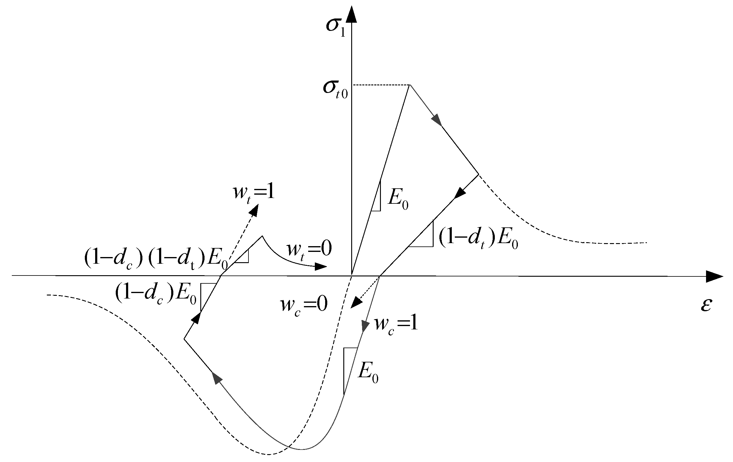
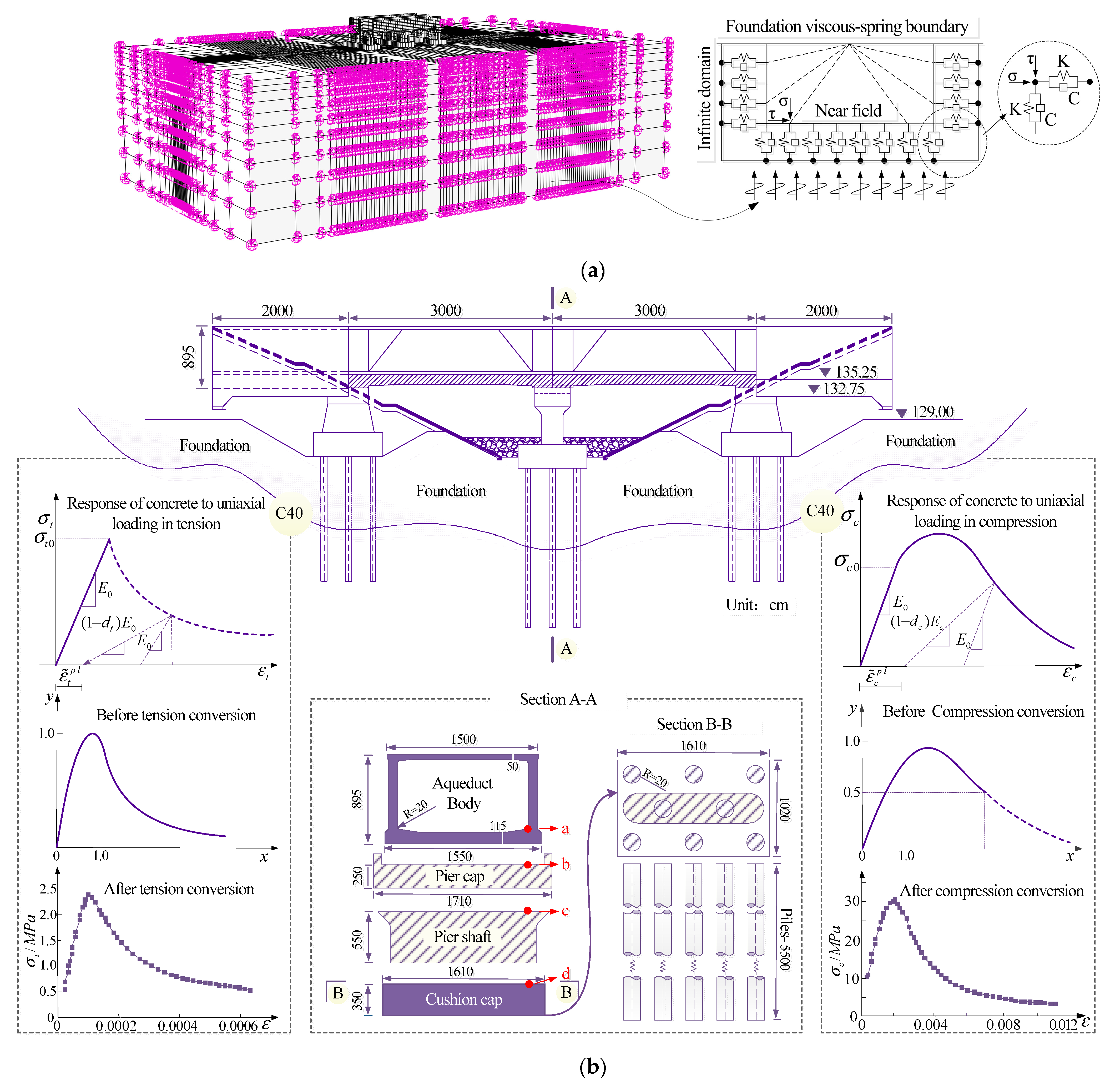
2.1. Concrete Damage Plasticity (CDP) Constitutive Model

The CDP constitutive model assumes that material is damaged by isotropic compression and tension. The damage factor d (Damage) is presented based on the plastic model to represent the irrecoverability of materials produced by damage to simulate the actual mechanical behavior of concrete [30,31]. It ranges from 0 (the material is not harmed) to 1 (the material is entirely destroyed). Based on the energy equivalent hypothesis, this study adapts Sidoroff’s [32] universal compression and tensile damage factor calculation approach and integrates it directly into the ABAQUS program. In Figure 1, taking C40 concrete as an example, the tensile-compression damage plastic parameters are calculated.

According to the plastic damage model theory in ABAQUS, the total strain tensor $\epsilon$ is composed of elastic strain rate ${\epsilon }^{el}$, and equivalent plastic strain rate ${\epsilon }^{\mathrm{pl}}$ can be determined as follows

$$\epsilon ={\epsilon }^{el}+{\epsilon }^{\mathrm{pl}}$$

(1)

When there is no damage to the concrete, the stress-strain relationship of the concrete is

$$\sigma =D^{el}(\epsilon -{\epsilon }^{\mathrm{pl}})$$

(2)

in which $\sigma$ is the total stress and $D^{el}$ is the elastic stiffness matrix. When the concrete is damaged, the material damage factor is introduced to describe the degradation of stiffness, and the relationship of damaged concrete in a three-dimensional multiaxial state can be expressed by the damage elastic equation:

$$\sigma =(1-d)\overline{\sigma }=(1-d)D_{}^{el}(\epsilon -{\epsilon }_{}^{\mathrm{pl}})$$

(3)

In this formula, $\overline{\sigma }$ is the effective stress, and d is the damage factor, which varies from 0 (no damage) to 1 (complete damage).

The complex damage mechanism of concrete under cyclic alternating stress is related to the cracking, consolidation, and changing of early cracks. When concrete is changed from tension to compression, the stiffness of the concrete recovers locally. To reflect the phenomenon, it is assumed that the relationship between the damage factor and tensile and compressive damage variables ($d_{\mathrm{t}}$ and $d_{\mathrm{c}}$) under an alternating load is

$$(1-d)=(1-s_{\mathrm{t}}{d}_{\mathrm{c}})(1-s_{\mathrm{c}}{d}_{\mathrm{t}}),0\le s_{\mathrm{t}},s_{\mathrm{c}}\le 1$$

(4)

where $s_{\mathrm{t}}$ and $s_{\mathrm{c}}$ are the relationship of stress action under stiffness recovery, which can be determined as follows

$$\{\begin{array}{l}{s}_{\mathrm{t}}=1-w_{\mathrm{t}}{r}^{\ast }(\overline{\sigma }),0\le w_{\mathrm{t}}\le 1\\ s_{\mathrm{c}}=1-w_{\mathrm{c}}(1-r^{\ast }(\overline{\sigma })),0\le w_{\mathrm{c}}\le 1\end{array}$$

(5)

where $r^{\ast }(\overline{\sigma })$ is the weight factor in the relationship of principal stress under a multiaxial state, which is

$$r^{\ast }(\overline{\sigma })\stackrel{\mathrm{def}}{=}\frac{{\displaystyle {\sum }_{i=1}^3\langle {\overline{\sigma }}_i\rangle }}{{\displaystyle {\sum }_{i=1}^3\left|{\overline{\sigma }}_i\right|}},0\le r^{\ast }(\overline{\sigma })\le 1$$

(6)

in which $w_{\mathrm{t}}$ and $w_{\mathrm{c}}$ are stiffness recovery weighting factors related to material properties. ${\overline{\sigma }}_i(i=1,2,3)$ is the main stress component; $\langle •\rangle$ can be expressed as

$$\langle x\rangle =\left(\left|x\right|+x\right)/2$$

Figure 1 shows the stiffness recovery curve of the concrete damage model under a uniaxial alternating load. The weight factors under tension and compression are ${\omega }_t=0$ (compression → tension) and ${\omega }_c=1$ (tension → compression), respectively.

The different evolution laws of material strength under tension and compression load are considered in the yield function of the CDP model, and the expression of effective stress is

$$F(\overline{\sigma },{\tilde{\epsilon }}^{\mathrm{pl}})=\frac{1}{1-\alpha }(\overline{q}-3\alpha \overline{p}+\beta ({\tilde{\epsilon }}^{\mathrm{pl}})\langle {\widehat{\overline{\sigma }}}_{\max }\rangle -\gamma \langle -{\widehat{\overline{\sigma }}}_{\max }\rangle )-{\overline{\sigma }}_{\mathrm{c}}({\tilde{\epsilon }}_{\mathrm{c}}^{\mathrm{pl}})\le 0$$

(7)

$$\begin{array}{l}\alpha =\frac{\left({\sigma }_{\mathrm{b}0}/{\sigma }_{\mathrm{c}0}\right)-1}{2\left({\sigma }_{\mathrm{b}0}/{\sigma }_{\mathrm{c}0}\right)-1}\left(0\le \alpha \le 0.5\right)\\ \beta ({\tilde{\epsilon }}^{\mathrm{pl}})=\frac{{\overline{\sigma }}_{\mathrm{c}}({\tilde{\epsilon }}_{\mathrm{c}}^{\mathrm{pl}})}{{\overline{\sigma }}_{\mathrm{t}}({\tilde{\epsilon }}_{\mathrm{t}}^{\mathrm{pl}})}(1-\alpha )-(1+\alpha )\\ \gamma =\frac{3\left(1-K_{\mathrm{c}}\right)}{2K_{\mathrm{c}}-1},\overline{p}=-\frac{1}{3}I:\overline{\sigma }\\ \overline{q}=\sqrt{\frac{3}{2}\overline{S}:\overline{S}},\overline{S}=\overline{p}I+\overline{\sigma }\end{array}\}$$

(8)

where $\alpha$ and $\gamma$ are dimensionless constants; ${\widehat{\overline{\sigma }}}_{\max }$ is the maximum effective principal stress; the effective hydrostatic pressure and Mises equivalent stress are $\overline{p}$ and $\overline{q}$; ${\sigma }_{\mathrm{b}0}$ is the equal axial initial yield stress, and ${\sigma }_{\mathrm{c}0}$ is the non-equiaxial initial yield stress; $K_{\mathrm{c}}$ is the parameter of the plane yield curve of deviatoric stress; $I$ is the unit matrix quantity; and $\overline{S}$ is the effective stress deviation.

The CDP model adopts the flow potential $G$ expression of the Drucker–Prager hyperbola as

$${\dot{\epsilon }}^{\mathrm{pl}}=\dot{\lambda }\frac{\partial G(\overline{\sigma })}{\partial \overline{\sigma }}$$

(9)

where $\dot{\lambda }$ is the plasticity factor, and $G$ is the Drucker-Prager hyperbolic formula, which can be expressed as

$$G=\sqrt{{(\in {\sigma }_{\mathrm{t}0}\tan \psi )}^2+{\overline{q}}^2}-\overline{p}\tan \psi$$

(10)

in which $\psi$ is the expansion angle in the meridian plane under a high confining pressure; ${\sigma }_{\mathrm{t}0}$ is the ultimate uniaxial tensile strength; and $\in$ is the variable of hyperbolic eccentricity, which is used to describe the rate at which the potential function approaches its asymptote.

2.2. Case Model

This paper takes an aqueduct of the SNWDP in China as an example. The body of the aqueduct is rectangular with a length of 60 m, with a bottom width of 15 m and a height of 8.95 m. The pier cap is 17.10 m long, 5.20 m wide, and 2.50 m high. The pier shaft is 5.50 m in height; and the pile cap is 16.10 m in length, 10.20 m in width, and 3.50 m in height. There were 71,172 three-dimensional solid elements used to build the body of the aqueduct and the foundation model. The model mainly uses the eight-node hexagonal Solid65 element, and the pull beam is simulated by the Beam 3 element (Figure 2). The main materials are shown in

Table 1. Various material parameters of the aqueduct.

Material	Elastic Modulus (GPa)	Density (Kg·m−3)	Poisson Ratio	Tensile Strength (MPa)	Compressive Strength (MPa)
Cushion caps(C30)	30.0	2385	0.167	1.43	14.3
Pier shafts/Pier caps(C40)	32.5	2400	0.167	1.71	19.1
Aqueduct body(C50)	34.5	2500	0.167	1.89	23.1

. In the dynamic calculation, an artificial viscous-spring boundary is applied to the foundation to simulate the seismic wave propagation process and reflect the energy dispersion at the boundary. The far boundary of the foundation is at a distance from the aqueduct of approximately 1.5~2 times the aqueduct in all directions. The dynamic response is analyzed by the commercial finite element software ABAQUS. In this study, a dynamic implicit analysis is performed.

For the seismic analysis of the aqueduct structure, natural frequencies and modes are usually used to study its vibration characteristics. In the solutions to most seismic problems, the first sloshing mode of a structure makes a dominant contribution to all the other modes [2]. The natural frequency of the aqueduct selected in this paper is 1.162 Hz when the design water level is 7.50 m.

Table 2. The first eight frequencies and vibration modes of the aqueduct structure.

Mode Number	Modal	Vibration Modes	Mode Number	Modal	Vibration Modes
1	1.162 Hz	Transverse	5	1.271 Hz	Vertical
2	1.168 Hz	Transverse	6	1.301 Hz	Vertical
3	1.197 Hz	Transverse	7	1.304 Hz	Transverse
4	1.214 Hz	Transverse	8	1.362 Hz	Vertical

shows the first eight vibration modes of the aqueduct structure. Compared to the natural frequencies of other aqueducts of similar height, width, and length under wet mode conditions, this aqueduct’s natural frequency and mode of vibration are similar to other aqueducts [33,34]. For example, the first natural frequency of an aqueduct (50 m × 14 m × 7 m) is 1.199 Hz [35]. We refer to the results of a doctoral dissertation. The aqueduct structure is similar to it in this paper (single 30 m × 20 m × 8 m) [35]. In the dynamic model experiment, the first frequency of modal identification is about 0.9~1.2 Hz, and the finite element calculation result is 0.973 Hz. Therefore, the natural frequency results of the aqueduct structure in this paper can be used to validate the accuracy of the finite element model. In this study, Rayleigh damping is used for the analysis, and the damping ratio corresponding to the structural frequency is taken as 5%, $\alpha =0.366$, and $\beta =0.007$.

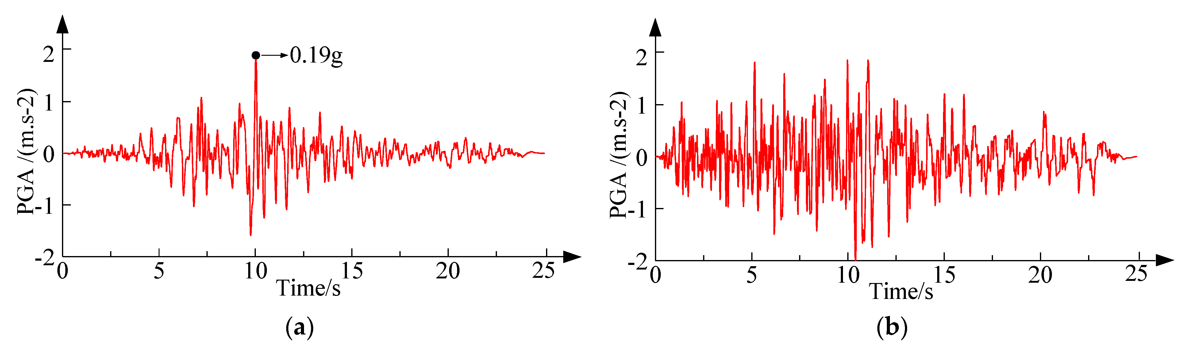
2.3. Ground Motion Input

The engineering foundation site classification is Class II, and the seismic intensity scale is VIII. To better understand the structural vibration response, damage development process, and damage degree caused by strong earthquakes, the data from the strong earthquake database of the Pacific Earthquake Engineering Research (PEER) Centre was used as a reference to select waves with a magnitude of 6~8, with shear wave velocity of 500~750 m/s, and epicentral distance of 0~105 km. The natural wave Northridge-01 (Whittier-S. Alta Dr), which was close to the characteristic site period of 0.4 s, has been chosen, following the frequency band fixation method proposed by the Applied Technology Council (ATC-3) in 1978 [36]. The basic parameters of selected natural waves are shown in

Table 3. Ground motion parameters of natural wave Northridge-01.

Earthquake Name	Station Name	EPA	EPV	Tg	βmax
Northridge−01	Whittier−S. Alta Dr	0.67	0.06	0.56	2.25

. The horizontal peak acceleration of severe earthquakes is 0.19 g, and the ratio to the vertical peak acceleration is 1:0.65. The seismic wave input interval is 0.01 s, and the total duration is 25 s. Two acceleration time−history curves are shown in Figure 3. The additional mass approach proposed by Westergaard in 1933 during a seismic study on the dam body is also used when considering the force of the seismic load on the water body [37].

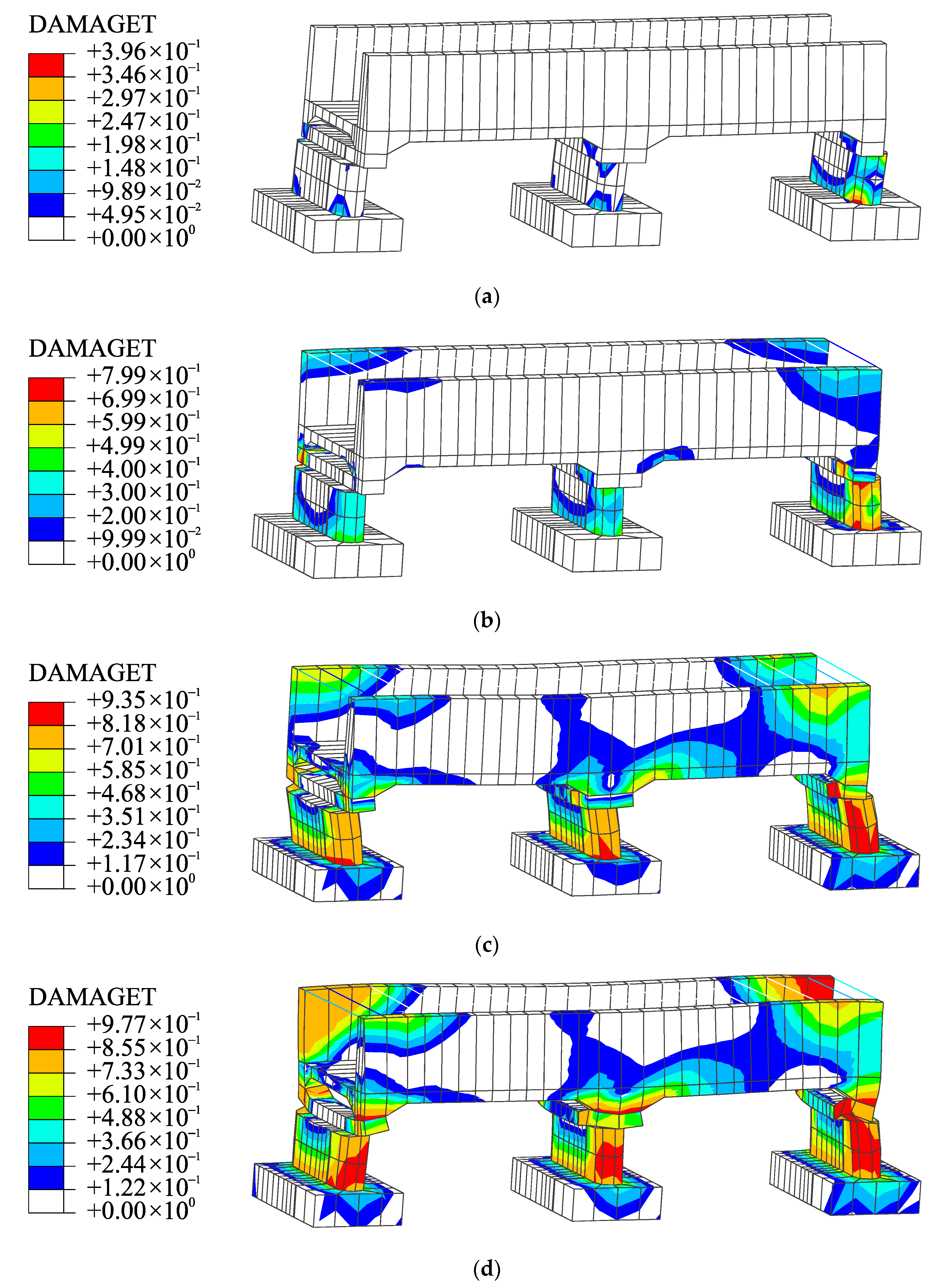
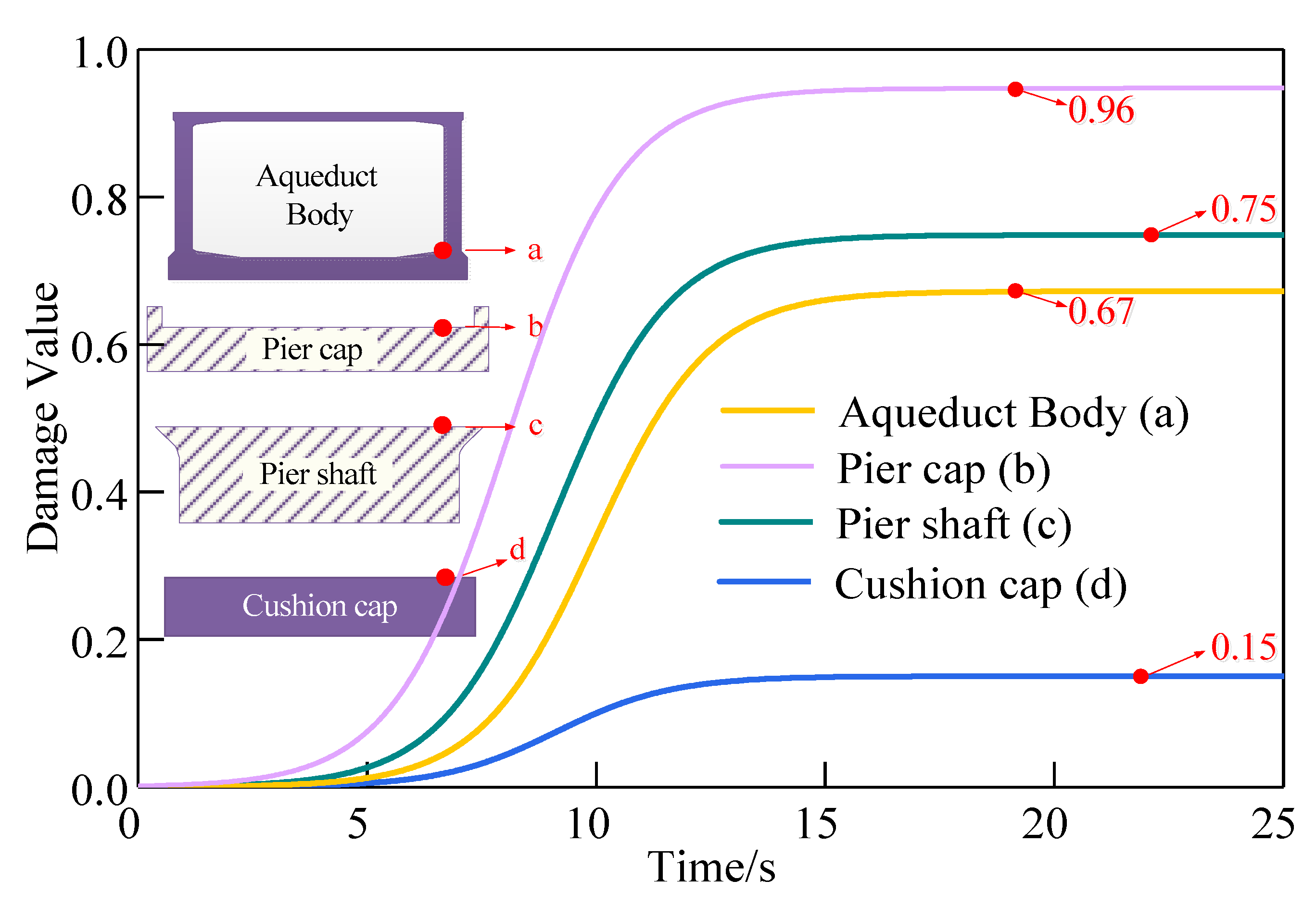
2.4. Damage Mechanism of Aqueduct Structures under Ground Motion

Figure 4 depicts the progression of the aqueduct structure’s dynamic damage as a result of significant earthquakes. The pier shaft and pier cap were severely damaged because they functioned as the principal supports. Penetrating damage occurred on both sides of the pier cap and around the pier shaft, and minor damage near the cushion cap, as indicated by the damage development range. Because of the aqueduct’s high rigidity, damage only emerged near the top. The damage development pattern shows that the seismic excitation was weak at the early stages of the earthquake, and the structure was in the elastic stage, implying that damage has little impact on the result. The damage first showed on both sides of the pier shaft and at the bottom of the pier cap when the earthquake struck 3.70 s. It is due to the introduction of CDP constitutive, which describes the phenomenon of the concrete structure after damage. The structure was undergoing irreversible plastic damage. The damage range extended on both sides of the pier shaft in both directions throughout 4.22 s~8.20 s, reaching from the top and bottom of the aqueduct body to the middle, as illustrated in Figure 4a–d. Penetrating damage appeared on both sides of the pier shaft and the pier cap almost simultaneously throughout 8.20 s~10.44 s. However, due to the effect of foundations, the aqueduct body and cushion cap showed damage later than the pier shafts and pier caps, and the damage expanded slower than the aqueduct body. The damage ranges gradually increased throughout the entire aqueduct during the period 11.00 s~25.00 s, under the continuous action of the seismic force, as shown in Figure 4c,d. At the later stage of the earthquake, the damage ranges eventually stabilized when the earthquake duration curve shifted.

Changes in acceleration cause the structural stress state to vary during the seismic wave motion process, an important component of dynamic load time history calculation. The feature points on one side of the structure are chosen for analysis to examine the development process and laws of aqueduct structural damage during seismic wave motion. Figure 5 depicts the evolution and changes in damage value at each point. The slope of the damage development process curve of the pier cap is the largest, and it is also the position where the damage occurs first. The damage range quickly increases over the entire aqueduct construction as the seismic force continues, and the pier shaft and pier cap are damaged almost simultaneously, and entirely. Compared to the pier shaft and pier cap, the cushion cap is damaged later and has a smaller damage range.

The damage to the aqueduct structure proliferates, as evidenced by the damage development curves of characteristic points. The structural damage aggravates rapidly when the ground motion acceleration reaches its peak, indicating that the peak acceleration of ground motion can considerably impact the damage to the structure, and the seismic damage is severe. When comparing the development trend of damage to various elements, pier caps and pier shafts exceed the aqueduct body and cushion caps significantly. Since pier shafts and pier caps are responsible for sustaining the upper structure and affecting its overall stability, it is hypothesized that the rapid progression of damage to pier shafts and pier caps is due to their increased displacement under seismic forces. The above assessments show that the most susceptible parts of the aqueduct are the pier tops and pier shafts, followed by the top of the aqueduct body, which should be the focus of concern during a strong earthquake. The entire aqueduct structure may collapse if the damage and cracks are severe.

As can be seen from the above analysis results, each element of the aqueduct structure is damaged to varying degrees when subjected to the action of a rare earthquake. The arrival time and intensity of earthquakes will occur randomly in real-world engineering. Earthquakes of various magnitudes have also struck places where earlier seismic disasters have happened. The occurrence of these earthquakes of varying magnitudes is also likely to cause structural damage. So far, the fragility mechanism of aqueduct structures at various earthquake intensities has remained mostly unexplored. In the following section, we proceed to analyse the seismic fragility of an aqueduct using the IDA and MSA fragility methodologies, respectively, to verify the accuracy of fragility research results and provide a foundation for aqueduct seismic research and post-earthquake decision-making.

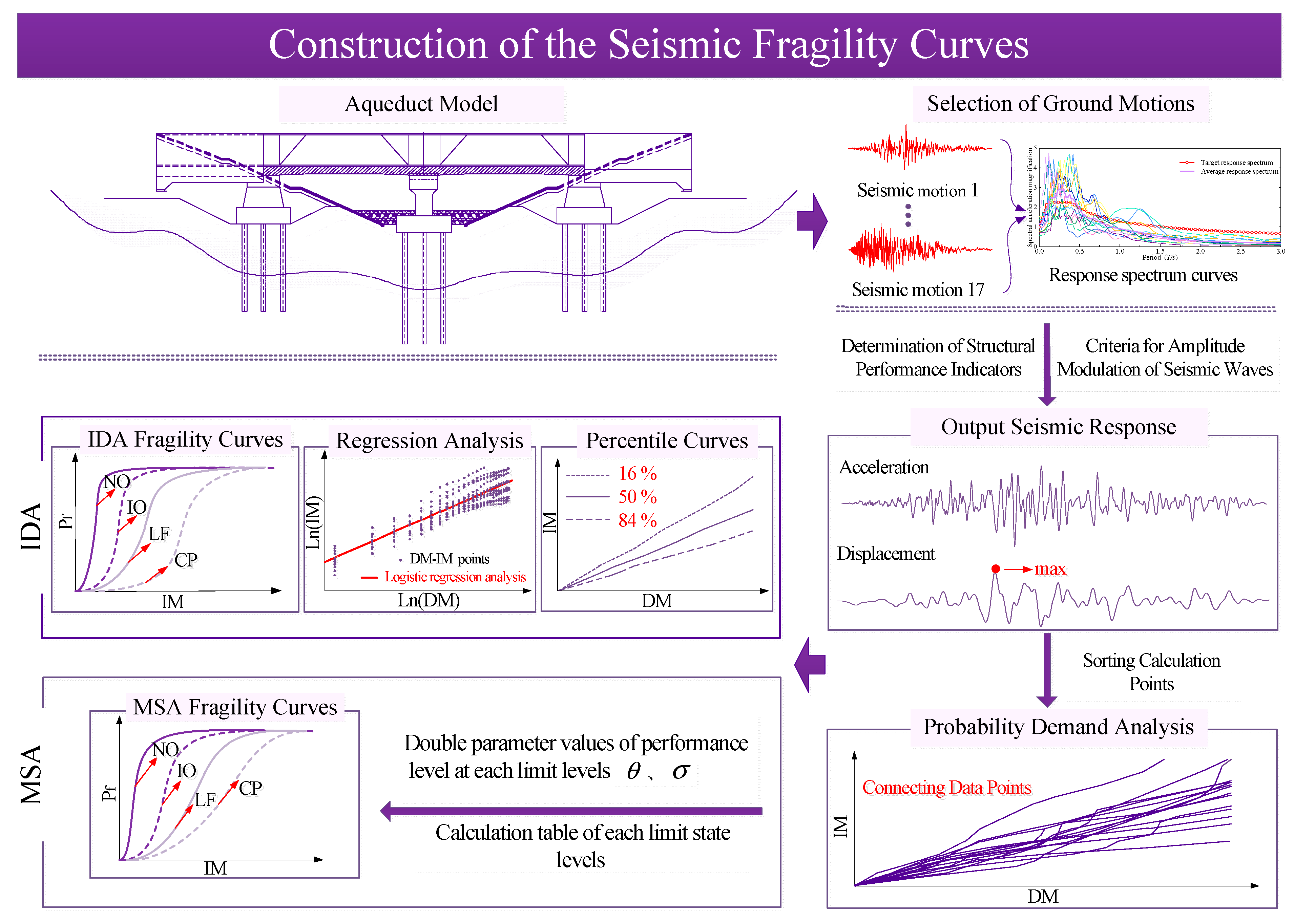
3. Seismic Fragility Analysis of the Aqueduct Structure

3.1. Methods to Develop Fragility Curves

To understand the importance of using the fragility functions and how scholars can be used to assess various structures against earthquakes, this section presents the fragility function types and the difference between them.

The fragility curves are an important tool to assess seismic risk. Every building or structure has its fragility curve. Based on the literature review [38], four methods to develop fragility curves can be identified, namely: (1) expert-based method; (2) empirical; (3) analytical; (4) hybrid.

(1) Expert-Based Method: The expert-based method is the oldest and simplest one among those mentioned above. This method depends on the use of questionnaires, the experiences of experts, and the number of experts consulted. In general, their judgments or opinions may contain uncertainties and may be less accurate, thus affecting the quality of the result.

(2) Empirical: The fragility curve developed by this empirical method is based on previous earthquake events. The advantage of this approach is that it shows the actual fragility to represent a realistic picture.

(3) Analytical: This approach is developed using simulated data from a time history analysis of the structural model for real. The analytical method is the most popular method in developing fragility seismic curves because this approach has less bias. The weakness of the analytical method is its requirement to produce a realistic model, that is, if the model is improperly designed or unrealistic, then it may result in inaccurate estimation that can affect the fragility curve.

(4) Hybrid: the hybrid approach is a calibrated empirical and analytical method, and is conducted by integrating numerical method to solve a numerical structural model equation. The disadvantage of the hybrid method is that it requires the combination of experiment and analysis.

3.2. Basic Principles of Incremental Dynamic Analysis (IDA)

The numerical method is commonly used in the seismic fragility analysis of a structure. That is, if a house fails to withstand an earthquake and collapses totally, the fragility probability is 1; if the house remains intact, the likelihood is 0. The relationship between the structural engineering demand measure (DM) and the seismic intensity measure (IM) in fragility analysis is

$$DM=\alpha {(IM)}^{\beta }$$

(11)

Assuming the median $\overline{D}$ of the seismic demand parameter and that the seismic intensity measure is subject to an exponential relationship, which is

$$\overline{D}=\alpha {(IM)}^{\beta }$$

(12)

Take logarithms of both sides of the above formula to get, where a and b are regression coefficients,

$$Ln\overline{D}=a+bLn{(IM)}^{\beta }$$

(13)

$\mathrm{Let}{\lambda }_d=Ln\overline{D},\mathrm{then}$

$${\beta }_d=\sqrt{\frac{1}{N-2}{\displaystyle \sum _{i-1}^N(Ln(DM)-Ln(\overline{D}))}}$$

(14)

In the formula, ${\lambda }_d$ is the logarithmic mean of $DM$; and ${\beta }_d$ is the logarithmic standard deviation of $DM$.

Define the capacity parameter $C$ of the structure with the logarithmic mean ${\lambda }_d$ and logarithmic standard deviation ${\beta }_d$; then:

$$P_f=P(C/D<1)$$

(15)

That is, $P_f=P(C-D<0)$. If $Z=C-D$, $C$ and $D$ are both independent random variables and subject to normal distribution so that $Z$ is also subject to normal distribution, and its mean is ${\lambda }_z={\lambda }_c-{\lambda }_d$ and standard deviation ${\beta }_z=\sqrt{{\beta }_c^2+{\beta }_d^2}$. The exceedance probability $P_f$ for a certain performance level of a structure under a specific action of earthquakes can be expressed as:

$$P_f=\Phi (-\frac{{\lambda }_c-{\lambda }_d}{\sqrt{{\beta }_c^2+{\beta }_d^2}})=\Phi (-\frac{Ln(\overline{C}/\overline{D})}{\sqrt{{\beta }_c^2+{\beta }_d^2}})=\Phi (\frac{Ln(\overline{D}/\overline{C})}{\sqrt{{\beta }_c^2+{\beta }_d^2}})$$

(16)

3.3. Basic Principles of Multiple Strip Analysis (MSA)

According to reference [26], $\theta$ and $\sigma$ are obtained through the maximum likelihood estimation (MLE) method to represent the logarithmic mean and logarithmic standard deviation of each performance state. The two-parameter ($\sigma$ and $\theta$) log-normal distribution function for the seismic fragility is:

$$P(C|IM=x)=\Phi (\frac{\ln x/\theta }{\sigma })$$

(17)

where $IM=x$ is the seismic intensity measure, $P(C|IM=x)$, represents the probability of the structure reaching a certain performance criterion when the input seismic intensity $IM=x$, and $\Phi (x)$ represents the standard normal distribution function. With the two parameters $\theta$ and $\sigma$, the normal distribution function with the seismic intensity measure $IM$ as an independent variable can be obtained for the fragility analysis

$$P(z_i)=\left(\begin{array}{c}{n}_i\\ z_i\end{array}\right)p_i{}^{z_i}{(1-p_i)}^{n_i-z_i}$$

(18)

According to the MLE principle and formula (18), the parameters $\theta$ and $\sigma$ are estimated thus:

$$L\left(\begin{array}{c}\theta \\ \sigma \end{array}\right)={\displaystyle \prod _{i=1}^{m}P(z_i)}={\displaystyle \prod _{i=1}^m\left(\begin{array}{c}{n}_i\\ z_i\end{array}\right)}{p}_i{}^{z_i}{(1-p_i)}^{n_i-z_i}$$

(19)

$$L\left(\begin{array}{c}\theta \\ \sigma \end{array}\right)={\displaystyle \prod _{i=1}^m\left(\begin{array}{c}{n}_i\\ z_i\end{array}\right)}\Phi {\left(\frac{ln(x_i/\theta )}{\sigma }\right)}^{z_i}{(1-\Phi \left(\frac{ln(x_i/\theta )}{\sigma }\right))}^{n-z_i}$$

(20)

$$\left\{\widehat{\theta },\widehat{\sigma }\right\}=\arg \max {\displaystyle \sum _{i=1}^m\left\{ln\left(\begin{array}{c}{n}_i\\ z_i\end{array}\right)+z_{i}ln\Phi \left(\frac{ln(x_i/\theta )}{\sigma }\right)+(n_i-z_i)ln\left[1-\Phi \left(\frac{ln(x_i/\theta )}{\sigma }\right)\right]\right\}}$$

(21)

Figure 6 illustrates the process for generating fragility curves. The engineering demand measure and the seismic intensity measure for aqueduct structure are estimated from the IDA, and the double parameter values of performance level at each limit state are calculated from the MSA.

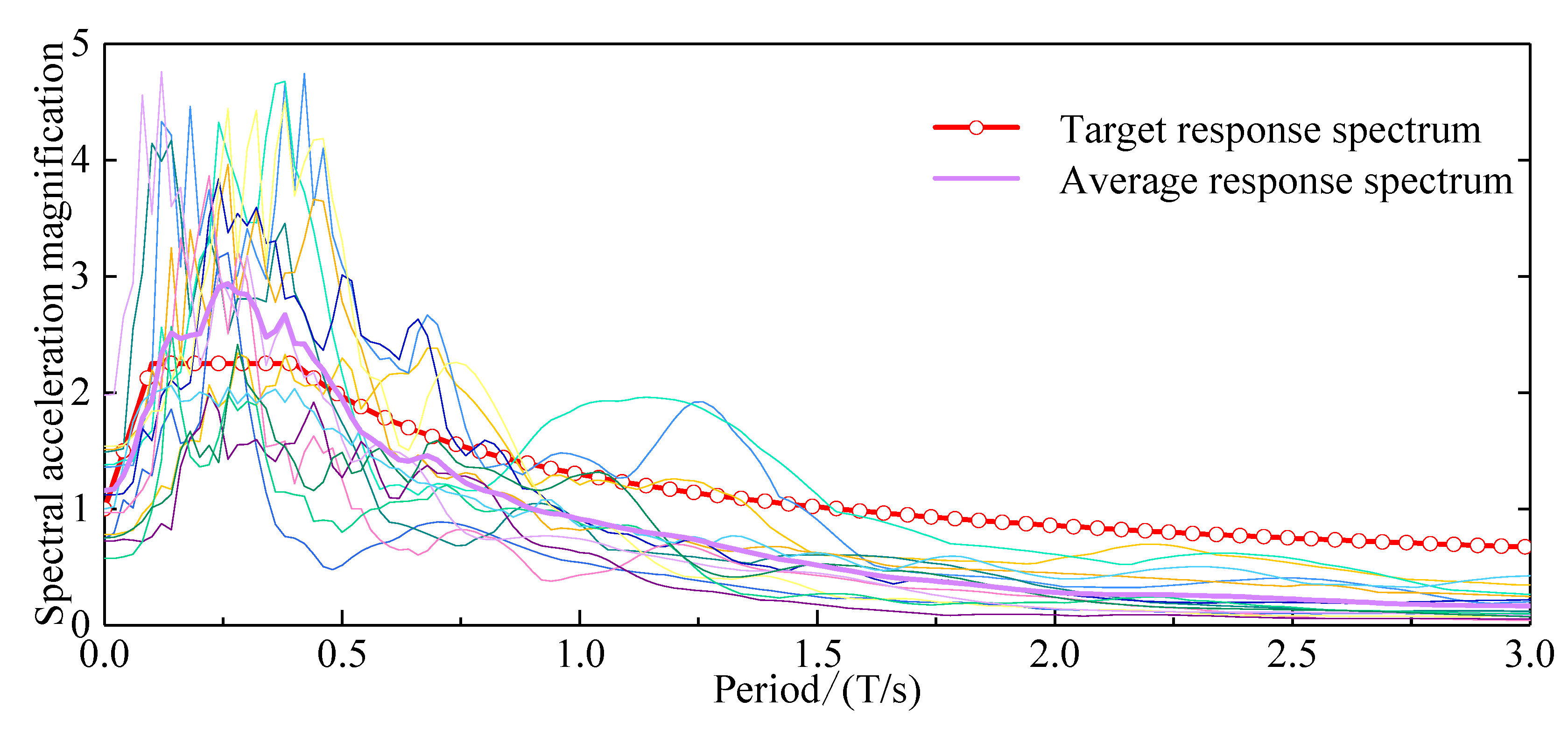
3.4. Selection of Ground Motions

Luco et al. [39] discovered that 10~20 seismic wave records might be used to estimate the structural earthquake-resistant capabilities of mid- to high-rise buildings correctly. Refer to Section 2.3 of this study for seismic wave selection criteria, and use the duration to attain 1/10 of the peak acceleration as the threshold [40]. Fifteen natural seismic waves from the database were chosen, along with two artificial waves that matched the engineering site spectrum.

Table 4. Ground-motion records for 6.0 ≤ M ≤ 8.0 and 0 ≤ R ≤ 105 km.

No.	Event	Station	M	R (km)	Time (s)	Mech	Year
1	San Fernando	Fairmont Dam	6.61	25.58	0.01	RN	1971
2	Taiwan SMART1(45)	SMART1 E02	7.3	51.35	0.01	RN	1986
3	Christchurch-New Zealand	MQZ	6.2	13.91	0.02	RO	2011
4	Coalinga-01	Parkfield-Fault Zone 11	6.36	27.1	0.01	RN	1983
5	Coalinga-01	Parkfield-Gold Hill 3W	6.36	38.1	0.01	RN	1983
6	Coalinga-01	Parkfield-Stone Corral 3E	6.36	32.81	0.01	RN	1983
7	Northridge-01	Burbank-Howard Rd	6.69	15.87	0.01	RN	1994
8	Northridge-01	Baldwin Park-N Holly	6.69	47.72	0.01	RN	1994
9	Northridge-01	Rancho Palos Verdes-Hawth	6.69	48.02	0.02	RN	1994
10	Northridge-01	Rancho Palos Verdes-Luconia	6.69	50.47	0.01	RN	1994
11	Northridge-01	Lake Hughes #4-Camp Mend	6.69	31.27	0.01	RN	1994
12	Northridge-01	Whittier–S.Alta Dr	6.69	48.36	0.01	RN	1994
13	Duzce-Turkey	Lamont 531	7.14	8.03	0.01	SS	1999
14	San Fernando	Lake Hughes#4	6.61	19.45	0.01	RN	1971
15	San Fernando	Pearblossom Pump	6.61	35.54	0.01	RN	1971
16	RHITG040	-	-	-	-	-	-
17	THITG040	-	-	-	-	-	-

Note: R: epicentral distance; M: moment magnitude; Mech: focal mechanisms; SS: strike slip; RN: reverse thrust; RO: reverse oblique.

lists the 17 seismic records, whereas Figure 7 depicts the response spectrum. The red line represents the target response spectrum.

3.5. Determination of Structural Performance Indicators

Studies have shown that PGA, PGV, and spectral acceleration S_a(T₁, 5%) can serve as common ground motion intensity measures [41,42,43]. Yu [44] chose 60 ground motion IM related to structural performance to construct ground motion parameter evaluation models. He believes that the analysis results involving the spectral acceleration could accurately describe the probability statistic relationship between IM and DM and avoid dispersion between analysis results. The aqueduct structure is similar to bridge structures in terms of engineering design. The pier shaft is responsible for sustaining the superstructure and affecting the overall stability of both structures. Bridge damage can be measured using a variety of indicators, including pier top displacement, pier top offset ratio, cracking degree, curvature ductility ratio, and displacement ductility ratio. Dutta and Mander [45] proposed the pier top offset ratio during their research, using it to indicate the pier shaft’s deformation capacity. It is the ratio of the maximum displacement of the pier top to the pier shaft height during the earthquake. The limit values are shown in

Table 5. Values of quantitative indexes correspond to structural performance levels.

Limit States	Damage Description	Discriminant Rule	Dr (m)	Umax (m)
(NO)	No or few structural and non-structural members are damaged.	θmax ≤ LS1	<0.007	<0.0385
(IO)	Minor repair is needed for structural and non-structural members.	LS1 ≤ θmax ≤ LS2	0.007~0.015	0.0385~0.0825
(LF)	The structure remains stable and has enough capacity.	LS2 ≤ θmax ≤ LS3	0.015~0.025	0.0825~0.1375
(CP)	The structure does not collapse and the damage is acceptable.	LS3 ≤ θmax ≤ LS4	0.025~0.050	0.1375~0.2750

Note: dr = U_max/H, dr is the aqueduct pier top offset ratio, U_max is the maximum displacement of aqueduct pier shaft top, and H is the height of aqueduct pier shaft, H = 5.5 m.

. The joint rotation features, structural damage degree, and deformation performance in the dynamic analysis are all directly related to displacement in the structure. Therefore, referring to the four limit states divided by FEMA356 and combined with the existing achievement of previous scholars [45,46,47], this paper divides structural earthquake-resistant performance into four grades: normal occupancy (NO), immediate occupancy (IO), life safety (LF), and collapse prevention (CP). We use the S_a(T₁, 5%) as ground motion IM and the aqueduct pier shaft top offset ratio to quantify the structural damage index limit to reflect the specific damage degree to a structure in case of exceedance probability. The limit state values of the quantitative indicators of the structural performance level can be found in Table 5.

3.6. Criteria for Amplitude Modulation of Seismic Waves

In this paper, the hunt and fill amplitude modulation criterion proposed by Vamvatasikos and Jalayer is used to balance the calculation accuracy and efficiency [48]. Using the natural wave Northridge-01 (Whittier–S. Alta Dr) as an example, we used the damping ratio of 5% to obtain the S_a(T₁, 5%) = 0.005 g at the first amplitude modulation, and a step increment of 0.05 g. The structure’s performance evolution law under ground motion excitation was determined progressively.

Table 6. Amplitude modulation calculation table.

Order Number	Calculation	Sa(T1, 5%) (g)	λ	Umax (m)
1	-	0.005	0.041	0.001
2	0.005 + 0.05	0.055	0.446	0.009
3	0.055 + 0.05 + 1 × 0.05	0.155	1.256	0.026
4	0.155 + 0.05 + 2 × 0.05	0.305	2.471	0.050
5	0.305 + 0.05 + 3 × 0.05	0.505	4.092	0.161
6	0.505 + 0.05 + 4 × 0.05	0.755	6.117	0.193
7	0.755 + 0.05 + 5 × 0.05	1.055	8.548	0.314
8	0.755 + (1.055 − 0.755)/3	0.855	6.928	0.255
9	0.505 + (0.755 − 0.505)/3	0.588	4.764	0.179
10	0.155 + (0.305−0.155)/3	0.205	1.661	0.034
11	0.055 + (0.155 − 0.055)/3	0.088	0.713	0.014
12	(0.755 + 0.505)/2	0.63	5.105	0.182
13	(0.505 + 0.305)/2	0.405	3.281	0.112
14	(0.305 + 0.155)/2	0.23	1.864	0.038
15	(0.155 + 0.055)2	0.105	0.851	0.017

depicts the exact amplitude modulation process.

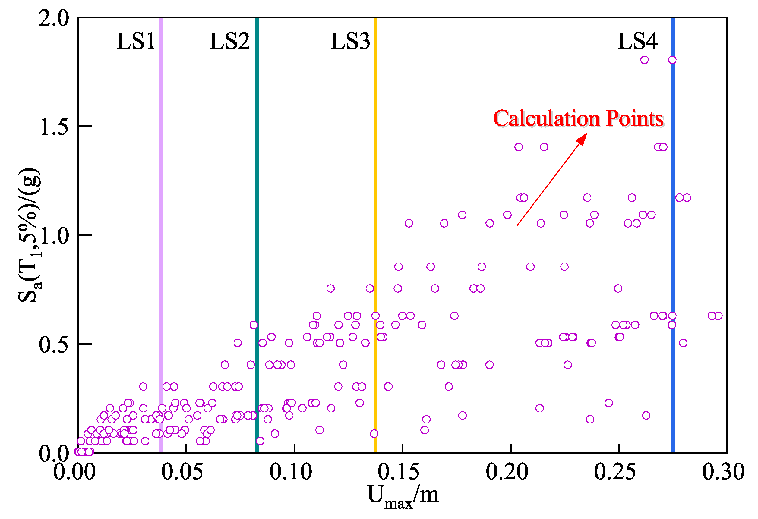
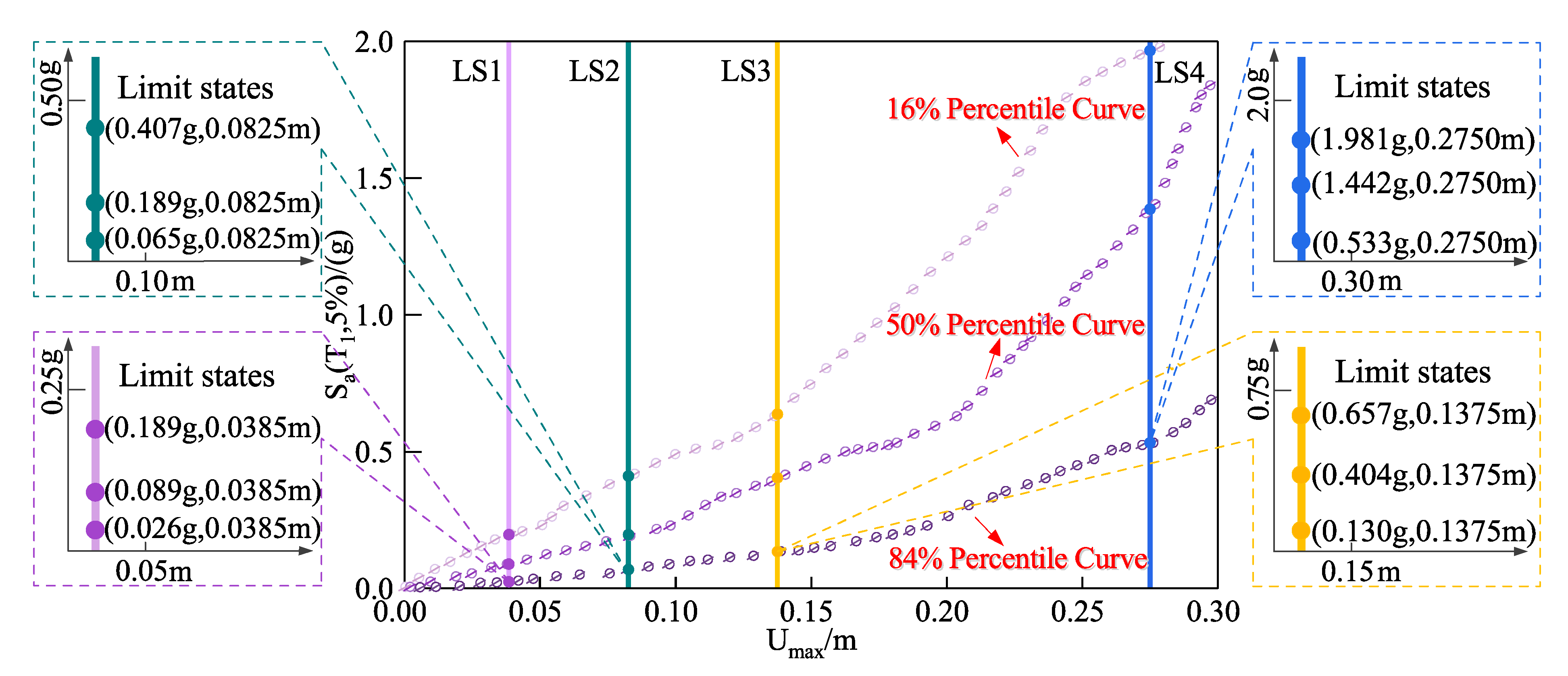
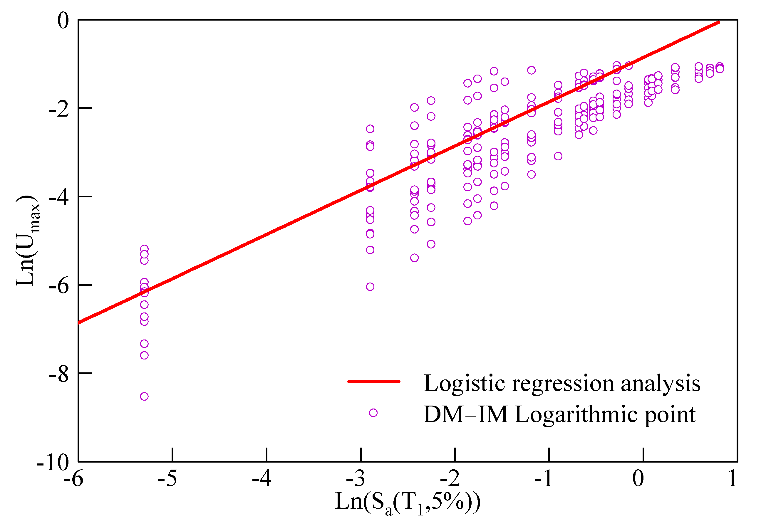
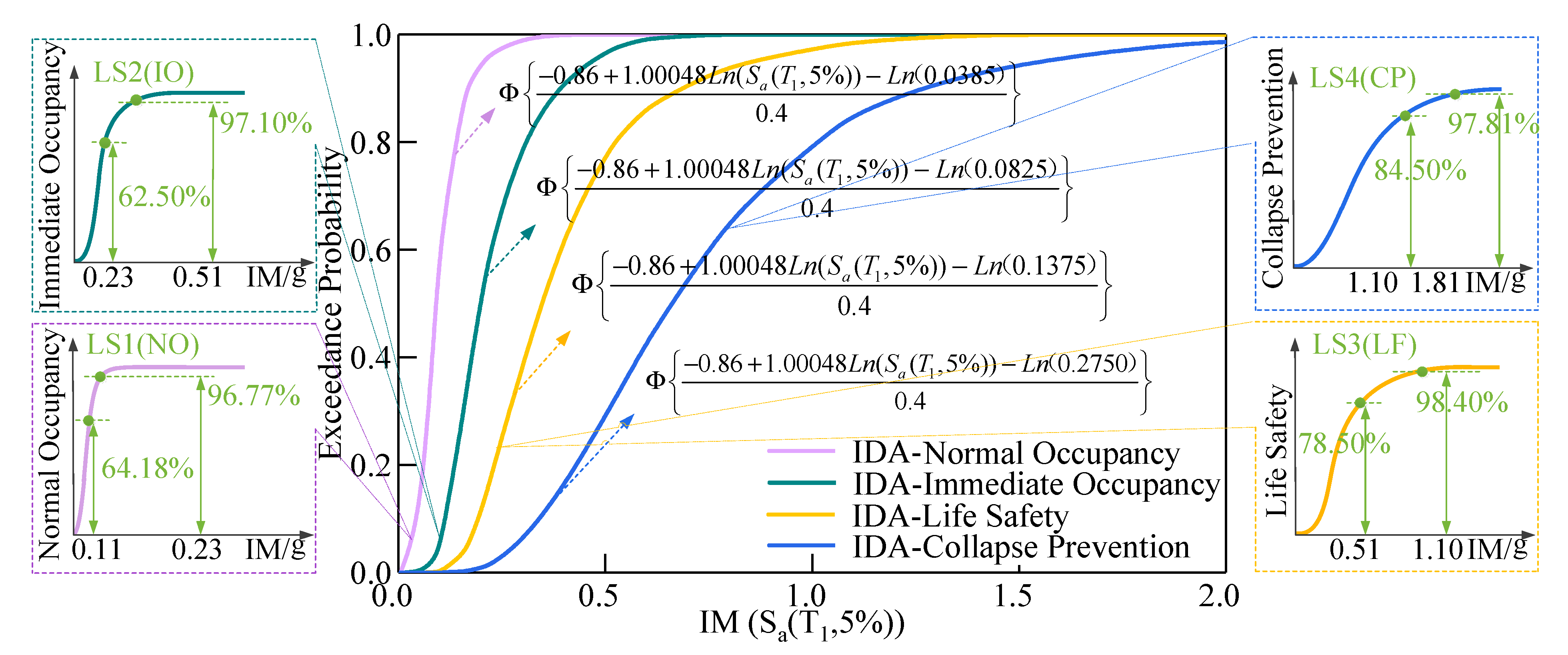
3.7. IDA Method-Based Probability Demand Analysis

Figure 8 depicts the results of a nonlinear analysis of the seismic dynamic response of an aqueduct structure under earthquake activity. When the IM remains constant, the data points in the graph reflect the maximum displacement of the pier shaft top of an aqueduct construction against different seismic waves. The quantitative indications of the four limit structural damage states are represented by the red dotted line. LS1 represents the limit state of the aqueduct structure changing from no damage to normal occupancy, LS2 represents the limit state of the aqueduct structure changing from normal occupancy to immediate occupancy, LS3 represents the limit state of the aqueduct structure changing from immediate occupancy to life safety, and LS4 represents the limit state of the aqueduct structure from life safety to collapse prevention.

Since a single IDA data cannot accurately predict the limit behavior of the structure, this paper selects a series of seismic records to perform the incremental dynamic analysis and obtain multiple IDA data. The 17 seismic ground records IDA data generated during ground motion excitation were summarized in the same IM-DM [(Umax–S_a(T₁, 5%))] coordinate system, as shown in Figure 8. It has been conducted using the same method as obtaining the IDA curve during ground motion excitation for the natural wave Northridge–01 (Whittier–S. Alta Dr). The response of the same structure to different seismic records input is discrete to some extent since the shape of the IDA curve is directly related to the selected seismic records. Therefore, it is necessary to summarize these different curves with the median and the 16% and 84% percentile curves to reduce the difference. The three IDA percentile curves obtained indicate that among the 17 seismic records, the 16%, 50%, and 84% seismic ground motion records exceeded the corresponding structural limit, as shown in Figure 9. The corresponding capacity values of each limit state of the structure are shown in

Table 7. Corresponding capacity values of each limit state of structure.

Limit States	IM(Sa(T1, 5%)) (g)			DM (Umax) (m)
	16%	50%	84%	16%	50%	84%
(NO)	0.189	0.089	0.026	0.0385	0.0385	0.0385
(IO)	0.407	0.189	0.065	0.0825	0.0825	0.0825
(LF)	0.657	0.404	0.130	0.1375	0.1375	0.1375
(CP)	1.981	1.442	0.533	0.2750	0.2750	0.2750

.

Taking the spectral acceleration S_a(T₁, 5%) as the independent variable IM and the maximum displacement of aqueduct pier shaft top as the dependent variable, the functional relation between them is as follows:

$$Ln(U_{\max })=a+bLn(S_a(T_1,5\%))$$

(22)

In the formula, $a$ and $b$ are regression coefficients. We performed a logarithmic regression analysis with the data in Figure 10, with a correlation coefficient R = 0.998. According to the seismic design standard HAZUS99 for building fragility curve parameters [49], when the fragility curve takes the spectral acceleration S_a(T₁, 5%) as the independent variable, $\sqrt{{\beta }_c^2+{\beta }_d^2}$ = 0.4. The functional relation is as follows:

$$Ln(U_{\max })=-0.86+1.00048Ln(S_a(T_1,5\%))$$

(23)

Figure 11 shows the seismic fragility curves of the aqueduct structure calculated based on the IDA method. For the limit state LS1, the IDA method obtains that the exceedance probability of the structure is 64.18% at 0.11 g and 96.77% at 0.23 g. In the limit state LS2, the exceedance probability of the structure at 0.23 g is 62.50%, and the exceedance probability at 0.51 g is 97.10%. According to the IDA method, when the structure is 0.51 g, the exceedance probability in LS3 is close to 80%. It implies that if the IM is greater than 0.50 g, the influence of weak structure components, such as the pier body and pier cap, should be adequately evaluated, as they are highly likely to affect structural safety. When the value exceeds 1.00 g, the probability is gradually close to 100%. In the LS4, the results show that the exceedance probability value of the structure is close to 90% at 1.10 g. The fragility analysis curve of the LS1 of the aqueduct structure under IDA conditions is highly steep and close to the vertical line, making it very simple to surpass the structural damage index of the LS1, according to studies on the characteristics of fragility curves. The LS2 has a somewhat steep fragility curve, while LS3 and LS4 gradually slow down. The IDA method is a traditional method to calculate the seismic fragility analysis curve of large buildings. The calculation of this method mainly depends on the logarithmic mean and logarithmic standard deviation of structural engineering demand parameters.

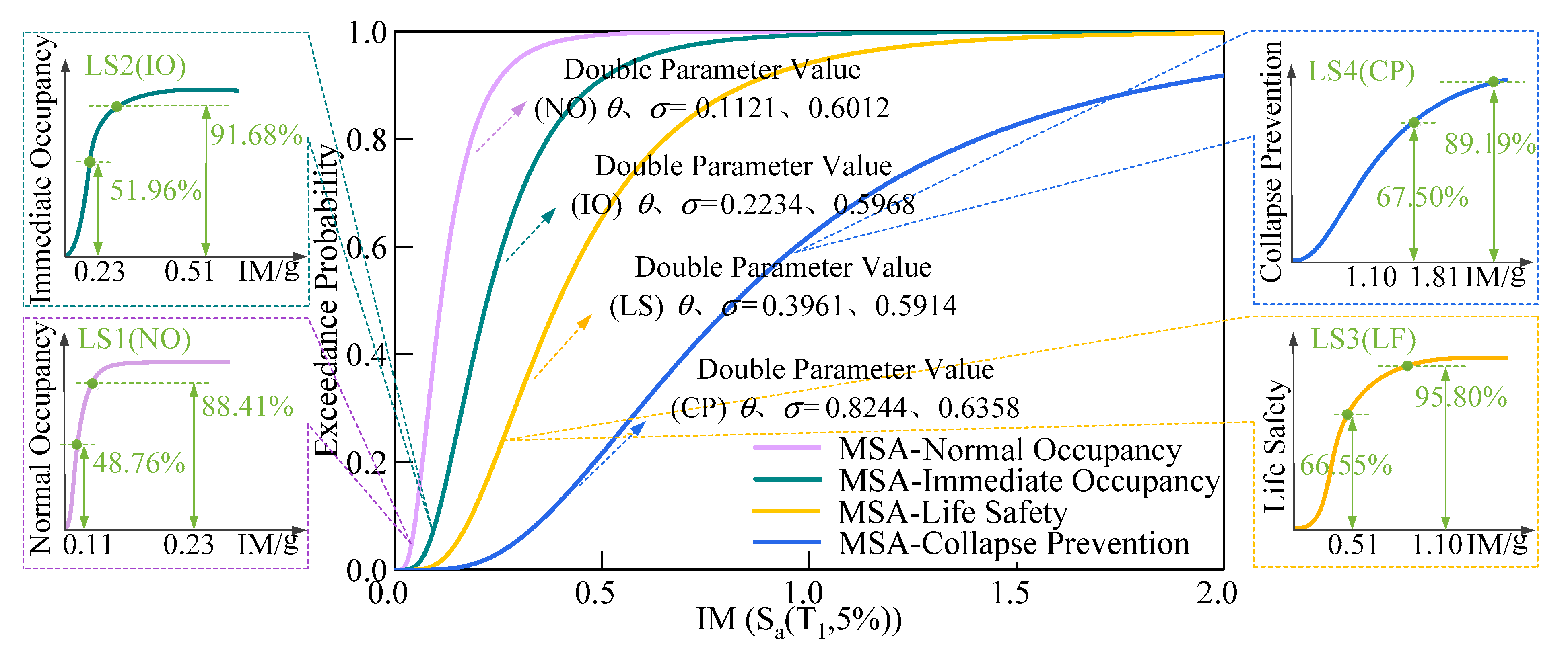
3.8. Determination of MSA-Based Performance Indicators of Each Limit State

Baker [50] found that the seismic data obtained using the IDA approach can likewise be used to generate seismic fragility curves using the MSA method. Based on Figure 10 and the basic principles of MSA, the double parameter values $\theta$ and $\sigma$ of each limit state performance level are obtained, as shown in

Table 8. Double parameter values of performance level at each limit state.

IM	Double Parameter Values
	(NO)		(IO)		(LF)		(CP)
$S_a(T_1,5\%)$	$\theta$	$\sigma$	$\theta$	$\sigma$	$\theta$	$\sigma$	$\theta$	$\sigma$
	0.1121	0.6012	0.2234	0.5968	0.3961	0.5914	0.8244	0.6358

.

Figure 12 shows the seismic fragility curves of the aqueduct structure calculated based on the MSA method. For limit state LS1, the exceedance probability of the structure is 48.76% at 0.11 g and close to 100% at 0.40 g based on the MSA method. The results show that the aqueduct structure selected in this paper is likely to produce small-scale damage when the IM exceeds 0.40 g. The fragility curve of the LS1 of the aqueduct structure is still very steep. In the LS2, the exceedance probability of the structure at 0.23 g is 51.96%, and at 0.51 g, the exceedance probability has reached 91.68%. It means that when the S_a(T₁, 5%) reaches 0.50 g, structures such as the pier shaft and pier cap are prone to damage. The pier cap and shaft of the aqueduct need repair, likely. In the limit state LS3, when the IM reaches 1.10 g, the exceedance probability is 95.80%, showing that the earthquake will cause serious damage to individual structural parts, affecting the safety and stability of the aqueduct structure.

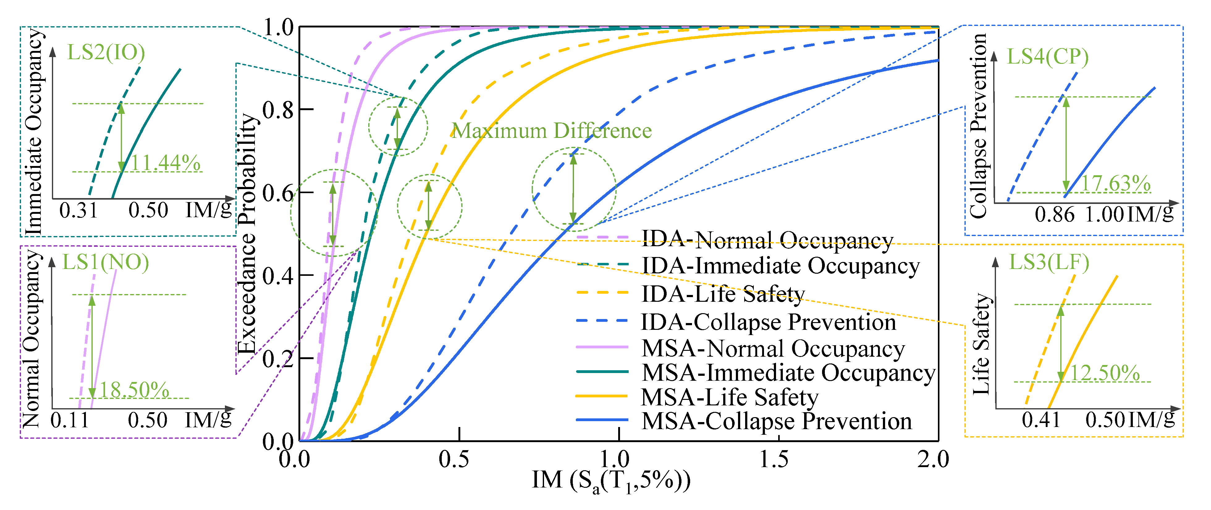
3.9. Comparison of Fragility Analysis Results of Aqueduct Structure

The comparison result of the two fragility curves based on the IDA and MSA methodologies is shown in Figure 13. Probability under various earthquake intensities is shown in

Table 9. Probability under various earthquake intensities (%).

Limit States	IM	0.00 5 g	0.05 5 g	0.08 8 g	0.10 5 g	0.15 5 g	0.17 2 g	0.20 5 g	0.23 0 g	0.30 5 g	0.40 5 g	0.50 5 g
LS1	IDA	0	10.49	46.88	64.18	86.99	91.20	94.98	96.77	99.40	99.99	100
	MSA	0	11.82	34.38	48.76	70.52	76.21	84.24	88.41	95.21	98.37	99.42
LS2	IDA	0	0	2.36	6.15	28.51	37.92	53.38	62.50	81.36	93.77	97.10
	MSA	0	0.94	5.92	11.76	27.02	33.07	44.29	51.96	69.92	84.07	91.68
LS3	IDA	0	0	0	0.24	3.25	5.65	12.59	19.55	41.35	64.89	78.50
	MSA	0	0	0	1.52	5.63	7.92	13.27	17.91	32.93	51.51	66.55
LS4	IDA	0	0	0	0	0.19	0.36	0.98	1.77	6.18	16.53	29.76
	MSA	0	0	0	0	0.43	0.72	1.43	2.23	5.89	13.10	22.50
Limit States	IM	0.53 3 g	0.58 8 g	0.63 0 g	0.75 5 g	0.85 5 g	1.05 5 g	1.09 4 g	1.17 2 g	1.40 5 g	1.80 5 g	2.03 5 g
LS1	IDA	100	100	100	100	100	100	100	100	100	100	100
	MSA	99.53	99.71	99.80	99.93	99.96	99.99	100	100	100	100	100
LS2	IDA	97.80	98.79	99.37	100	100	100	100	100	100	100	100
	MSA	92.75	94.76	95.89	97.93	98.78	99.54	99.62	99.73	99.90	100	100
LS3	IDA	81.78	85.40	87.75	92.70	95.23	97.65	98.40	99.10	99.90	99.99	100
	MSA	69.22	74.80	78.37	86.23	90.34	95.12	95.80	96.67	98.39	99.49	99.71
LS4	IDA	33.60	41.03	46.46	60.76	69.91	82.69	84.50	87.55	93.52	97.81	98.78
	MSA	24.64	29.75	33.61	44.50	52.29	65.10	67.50	71.00	79.92	89.19	92.18

. It can be seen that for LS1, the exceedance probability of the structure with IM = 0.11 g, the maximum difference of two fragility curves is about 18.50%, and their tendency is roughly in line. For LS2, the exceedance probability with IM = 0.31 g obtained by the two fragility methods is 81.36% and 69.92%, respectively. The IDA-based fragility curve has a steeper upward trend, with a difference of 11.44% between the two methods, and the two curves are in good agreement. The maximum difference for LS3 is about 12.50% for IM = 0.41 g. The maximum difference between LS4 and LS5 is 17.63%. The LS1 of the two methods shows a steep trend, and the fragility curves of the LS2 (slight damage) are also steep until the fragility curves of the LS3 and LS4 gradually slow down.

In conclusion, the seismic fragility curves generated using the IDA and MSA methodologies mutually verify the aqueduct structure’s seismic fragility results. The main reason for the large difference in the probability of individual damage is that MSA-based calculations are limited by the number of seismic waves exceeding the limit. In contrast, IDA-based calculations are based primarily on the mean and logarithmic standard deviation of the structural engineering demand parameter. However, their conclusions are largely in agreement, indicating that in the seismic analysis, the aqueduct structure will be difficult to maintain no damage, and it is very easy to exceed the damage index of the first limit state level. The IDA approach is very straightforward in theory in terms of calculation time, but it involves extensive calculations and complex data processing in practice. On the other hand, the MSA technique can provide the exceedance probability at any IM without complex work. In seismic calculations, IDA-based fragility analysis may fail to appropriately calculate the IM value corresponding to each limit state when the probability of the structure surpassing the damage index does not strictly increase with the IM positively. On the other hand, the MSA approach has no such flaws and can obtain multiple horizontal bands of IM-DM ground motion. The fragility curve is more precisely calculated using statistical analysis.

4. Conclusions

The dynamic damage mechanism and damage development law of an aqueduct under the impact of a rare earthquake are investigated in this research and the weak spots of the aqueduct structure where concrete cracking may occur. Seventeen seismic waves are selected based on the factors such as magnitude, shear wave velocity, epicentral distance, and site type. We use the IDA and MSA methods to analyze the seismic fragility of the aqueduct, respectively, with S_a(T₁, 5%) as the IM and the pier shaft top offset ratio under structural response to quantify the index limit, which mutually verifies the rationality of the fragility results and studies the probability of damage to the structure under different IM. The aqueduct selected in this paper is universal in the SNWDP. However, the aqueduct is located in an earthquake-prone area. The research results apply to the aqueduct, bridges, and other structures similar to the structural model and conditions in this paper. The following are the main conclusions:

• Penetrating damage is most likely to occur on both sides of the pier cap and around the pier shaft in the event of a rare earthquake, followed by the top of the aqueduct body, which will require the most concern during the earthquake. The entire aqueduct structure may collapse once the damage and cracks get severe. Therefore, in the process of seismic design, relevant damping measures should be taken to control the damage development and prevent the overall aqueduct structure from being damaged or collapsed. For easily damaged parts, appropriate structural reinforcement is required to meet the needs of earthquake resistance.
• Two fragility analysis methodologies are used to investigate the aqueduct structure separately. The results reveal that the fragility curves obtained by IDA and MSA are very similar. Except for individual results, the variation between fragility curves of different LS is less than 10%, demonstrating that the fragility analysis results are rational.
• Each of the two fragility methodologies has its advantages. The IDA method is simple in theory, but data processing is complicated because the logarithmic mean and logarithmic standard deviation for each seismic IM must be determined. In theory, the MSA method is more complicated, but the probability in the case of any IM may be calculated by acquiring only two parameters that correspond to the LS. In terms of calculation, it is more efficient.
• The seismic fragility analysis of aqueduct structure is the main research content in this paper. Although the fragility analysis of different methods is realized, this paper only selects one kind of spectral acceleration and the pier shaft top offset ratio under structural as the standard. The calculation index should be added to obtain the most suitable strength index and response index in the fragility study of the aqueduct, which will also be the next work of this research.
• The building needs need professional seismic hazard analysis, and the aqueduct structure is no exception. Combining with the research results of seismic fragility in this paper, constructing seismic hazard curves to jointly evaluate the seismic safety of the aqueduct structure is the next step of the authors.

References

1. Gonen, S.; Pulatsu, B.; Erdogmus, E.; Karaesmen, E.; Karaesmen, E. Quasi-Static Nonlinear Seismic Assessment of a Fourth Century A.D. Roman Aqueduct in Istanbul, Turkey. Heritage 2021, 4, 401–421. [Google Scholar] [CrossRef]
2. Li, Y.; Di, Q.; Gong, Y. Equivalent mechanical models of sloshing fluid in arbitrary-section aqueducts. Earthq. Eng. Struct. Dyn. 2011, 41, 1069–1087. [Google Scholar] [CrossRef]
3. Wu, Y.; Mo, H.; Yang, C. Study on dynamic performance of a three-dimensional high frame supported U-shaped aqueduct. Eng. Struct. 2006, 28, 372–380. [Google Scholar] [CrossRef]
4. Zhang, C.; Xu, J.; Wang, B.; Wu, C. Nonlinear random seismic response analysis of the double-trough aqueduct based on fiber beam element model. Soil Dyn. Earthq. Eng. 2021, 150, 106856. [Google Scholar] [CrossRef]
5. Ying, L.; Meng, X.; Zhou, D.; Xu, X.; Zhang, J.; Li, X. Sloshing of fluid in a baffled rectangular aqueduct considering soil-structure interaction. Soil Dyn. Earthq. Eng. 2019, 122, 132–147. [Google Scholar] [CrossRef]
6. Ding, X.; Yu, Q.; Wang, J. A numerical research on the aqueduct hydrodynamic pressure from earthquakes. Eur. J. Environ. Civ. Eng. 2013, 17, s229–s235. [Google Scholar] [CrossRef]
7. Knobloch, E. Review of Liquid Sloshing Dynamics: Theory and Applications. SIAM Rev. 2006, 48, 616–619. [Google Scholar]
8. Liu, Y.; Dang, K.; Dong, J. Finite element analysis of the aseismicity of a large aqueduct. Soil Dyn. Earthq. Eng. 2017, 94, 102–108. [Google Scholar] [CrossRef]
9. Zhang, H.; Sun, H.; Liu, L.; Dong, M. Resonance mechanism of wind-induced isolated aqueduct-water coupling system. Eng. Struct. 2013, 57, 73–86. [Google Scholar] [CrossRef]
10. Yazdani, M.; Jahangiri, V. Marefat M S. Seismic performance assessment of plain concrete arch bridges under near-field earthquakes using incremental dynamic analysis. Eng. Failure Anal. 2019, 106, 104170. [Google Scholar] [CrossRef]
11. Li, Y.; Lou, M.; Pan, D. Evaluation of vertical seismic response for a large-scale beam-supported aqueduct. Earthq. Eng. Struct. Dyn. 2002, 32, 1–14. [Google Scholar] [CrossRef]
12. Deierlein, G.G.; Krawinkler, H.; Cornell, C.A. A framework for performance-based earthquake engineering. In Proceedings of 2003 Pacific Conference on Earthquake Engineering; Elsevier: Christchurch, New Zealand, 2003; pp. 1–8. [Google Scholar]
13. Porter, K.A. An overview of PEER’s performance-based earthquake engineering methodology. In Proceedings of the Ninth International Conference on Applications of Statistics and Probability in Civil Engineering (ICASP9), San Francisco, CA, USA, 6–9 July 2003. [Google Scholar]
14. Moehle, J.; Deierlein, G.G. A framework methodology for performance-based earthquake engineering. In Proceedings of the 13th World Conference on Earthquake Engineering, Vancouver, BC, Canada, 1–6 August 2004. [Google Scholar]
15. Bertero, V.V. Strength and deformation capacities of buildings under extreme environments. Struct. Eng. Struct. Mech. 1977, 53, 29–79. [Google Scholar]
16. Vamvatsikos, D.; Cornell, C.A. Incremental dynamic analysis. Earthq. Eng. Struct. Dyn. 2002, 31, 491–514. [Google Scholar] [CrossRef]
17. Jalayer, F.; Cornell, C.A. A Technical Framework for Probability-Based Demand and Capacity Factor Design (DCFD) Seismic Formats; PEER Report 2003/08; Pacific Earthquake Engineering Research Center: Berkeley, CA, USA, 2004. [Google Scholar]
18. Crespi, P.; Zucca, M.; Valente, M. On the collapse evaluation of existing RC bridges exposed to corrosion under horizontal loads. Eng. Fail. Anal. 2020, 116, 104727. [Google Scholar] [CrossRef]
19. Crespi, P.; Zucca, M.; Longarini, N.; Giordano, N. Seismic Assessment of Six Typologies of Existing RC Bridges. Infrastructures 2020, 5, 52. [Google Scholar] [CrossRef]
20. Choi, E.; DesRoches, R.; Nielson, B. Seismic fragility of typical bridges in moderate seismic zones. Eng. Struct. 2004, 26, 187–199. [Google Scholar] [CrossRef]
21. Choe, D.-E.; Gardoni, P.; Rosowsky, D.; Haukaas, T. Probabilistic capacity models and seismic fragility estimates for RC columns subject to corrosion. Reliab. Eng. Syst. Saf. 2008, 93, 383–393. [Google Scholar] [CrossRef]
22. Argyroudis, S.; Pitilakis, K. Seismic fragility curves of shallow tunnels in alluvial deposits. Soil Dyn. Earthq. Eng. 2012, 35, 1–12. [Google Scholar] [CrossRef]
23. Mosalam, K.M.; Ayala, G.; White, R.N.; Roth, C. Seismic fragility of LRC frames with and without masonry infill walls. J. Earthq. Eng. 1997, 1, 693–720. [Google Scholar] [CrossRef]
24. Jalayer, F. Direct Probabilistic Seismic Analysis: Implementing Non-Linear Dynamic Assessments. Ph.D. Thesis, Stanford University, Stanford, CA, USA, 2003. [Google Scholar]
25. Jalayer, F.; Cornell, C.A. Alternative non-linear demand estimation methods for probability-based seismic assessments. Earthq. Eng. Struct. Dyn. 2009, 38, 951–972. [Google Scholar] [CrossRef]
26. Baker, J. Efficient Analytical Fragility Function Fitting Using Dynamic Structural Analysis. Earthq. Spectra 2015, 31, 579–599. [Google Scholar] [CrossRef]
27. Yuan, C.-Y. Study on the Structure-BCS Intelligent Control Methods for Mitigating the Vibration of Large-Scale Wind Turbines. Ph.D. Thesis, Dalian University of Technology, Liaoning, China, 2017. [Google Scholar]
28. Mahmoodi, K.; Noorzad, A.; Mahboubi, A.; Alembagheri, M. Seismic performance assessment of a cemented material dam using incremental dynamic analysis. Structures 2020, 29, 1187–1198. [Google Scholar] [CrossRef]
29. Gabbianelli, G.; Perrone, D.; Brunesi, E.; Monteiro, R. Seismic acceleration demand and fragility assessment of storage tanks installed in industrial steel moment-resisting frame structures. Soil Dyn. Earthq. Eng. 2021, 152, 107016. [Google Scholar] [CrossRef]
30. Lubliner, J.; Oliver, J.; Oller, S.; Oñate, E. A plastic-damage model for concrete. Int. J. Solids Struct. 1989, 25, 299–326. [Google Scholar] [CrossRef]
31. Xu, X.-Y.; Ma, Z.-Y.; Zhang, H.-Z. Simulation algorithm for spiral case structure in hydropower station. Water Sci. Eng. 2013, 6, 230–240. [Google Scholar] [CrossRef]
32. Sidoroff, F. Description of Anisotropic Damage Application to Elasticity. In Physical Non-Linearities in Structural Analysis, Proceedings of the IUTAM, Senlis, France, 27–30 May 1980; Hult, J., Lemaitre, J., Eds.; Springer: Berlin/Heidelberg, Germany; pp. 237–244. [CrossRef]
33. Liu, Y.; Zhang, B.; Chen, H. Aseismatic analysis of aqueduct structure for South to North Water Transfer Project. Water Resour. Hydropower Eng. 2004, 5, 49–51. (In Chinese) [Google Scholar]
34. He, J.-T. Fluid-Structure Dynamic Coupling’s Analysis of Large Scale Aqueduct. Master’s Thesis, Xi’an University of Technology, Xi'an, Shanxi, China, 2007. [Google Scholar]
35. Zhou, Z.-G. Study on the Pile-Soil-Aqueduct Interaction by Pseudo-Dynamic Test and Computational Analysis. Ph.D. Thesis, Hunan University, Changsha, Hunan, China, 2014. [Google Scholar]
36. Applied Technology Council. Tentative Provisions for the Development of Seismic Regulations for Buildings: A Cooperative Effort with the Design Professions, Building Code Interests and the Research Community; U.S. Department of Commerce, National Bureau of Standards: Washington, DC, USA, 1978. [Google Scholar]
37. Westergaard, H.M. Water Pressures on Dams during Earthquakes. Trans. Am. Soc. Civ. Eng. 1933, 98, 418–433. [Google Scholar] [CrossRef]
38. Nazri, F.M. Seismic Fragility Assessment for Buildings Due to Earthquake Excitation; Springer: Singapore, 2018. [Google Scholar]
39. Luco, N.; Cornell, C.A. Effects of Connection Fractures on SMRF Seismic Drift Demands. J. Struct. Eng. 2000, 126, 127–136. [Google Scholar] [CrossRef]
40. Kanai, K. Engineering Seismology; University of Tokyo Press: Tokyo, Japan, 1983. [Google Scholar]
41. Shinozuka, M.; Feng, M.Q.; Lee, J.; Naganuma, T. Statistical Analysis of Fragility Curves. J. Eng. Mech. 2000, 126, 1224–1231. [Google Scholar] [CrossRef] [Green Version]
42. Alam, M.S.; Bhuiyan, M.A.R.; Billah, A.H.M.M. Seismic fragility assessment of SMA-bar restrained multi-span continuous highway bridge isolated by different laminated rubber bearings in medium to strong seismic risk zones. Bull. Earthq. Eng. 2012, 10, 1885–1909, Erratum in 2012, 10, 1911–1913. [Google Scholar] [CrossRef]
43. Asteris, P.; Chronopoulos, M.; Chrysostomou, C.; Varum, H.; Plevris, V.; Kyriakides, N.; Silva, V. Seismic vulnerability assessment of historical masonry structural systems. Eng. Struct. 2014, 62–63, 118–134. [Google Scholar] [CrossRef]
44. Yu, X.-H. Probabilistic Seismic Fragility and Risk Analysis of Reinforce Concrete Frame Structures. Ph.D. Thesis, Harbin Institute of Technology, Harbin, China, 2012. [Google Scholar]
45. Dutta, A.; Mander, J. Rapid and Detailed Seismic Fragility Analysis of Highway Bridges; Technical Report for Multidisciplinary Center for Earthquake Engineering: Buffalo, NY, USA, 2002. [Google Scholar]
46. American Society of Civil Engineers. Prestandard and Commentary for the Seismic Rehabilitation of Buildings; FEMA 356, Technical report for Federal Emergency Management Agency; FEMA: Washington, DC, USA, 2000; pp. 55–57. [Google Scholar]
47. Liu, J.; Liu, Y.; Liu, H. Seismic fragility analysis of composite frame structure based on performance. Earthq. Sci. 2010, 23, 45–52. [Google Scholar] [CrossRef] [Green Version]
48. Vamvatsikos, D. Seismic Performance, Capacity and Reliability of Structures as Seen Through Incremental Dynamic Analysis. Ph.D. Thesis, Stanford University, Stanford, CA, USA, 2002. [Google Scholar]
49. FEMA: HAZUS99 Technical Manual; Federal Emergency Management Agency: Washington, DC, USA, 1999.
50. Baker, J.W. Probabilistic structural response assessment using vector-valued intensity measures. Earthq. Eng. Struct. Dyn. 2007, 36, 1861–1883. [Google Scholar] [CrossRef]
Figure 1. The stress–strain relationship under uniaxial load cycle conditions. ( ω t = 0 , ω t = 1 ).
Applsci 11 11709 g001
Figure 2. Aqueduct structure model. (a) Numerical model of the aqueduct structure; (b) Aqueduct structure details. a, b, c, and d are feature points of damage.
Applsci 11 11709 g002
Figure 3. Time history records of seismic accelerations. (a) Transverse; (b) Vertical.
Applsci 11 11709 g003
Figure 4. Developing process of aqueduct’s damage process under rare earthquake. (a) t = 4.22 s; (b) t = 8.20 s; (c) t = 10.44 s; (d) t = 25.00 s.
Applsci 11 11709 g004
Figure 5. Damage development process.
Applsci 11 11709 g005
Figure 6. Illustration of the steps for generating fragility curves.
Applsci 11 11709 g006
Figure 7. Response spectrum curves.
Applsci 11 11709 g007
Figure 8. Non-linear time history calculation points of 17 seismic waves.
Applsci 11 11709 g008
Figure 9. Percentile curves (IDA).
Applsci 11 11709 g009
Figure 10. Logistic regression analysis (IDA).
Applsci 11 11709 g010
Figure 11. Fragility curves (IDA).
Applsci 11 11709 g011
Figure 12. Fragility curves (MSA).
Applsci 11 11709 g012
Figure 13. Comparison of IDA and MSA.
Applsci 11 11709 g013