A Novel Method for Predicting Local Site Amplification Factors Using 1-D Convolutional Neural Networks

Abstract

The analysis of site seismic amplification characteristics is one of the important tasks of seismic safety evaluation. Owing to the high computational cost and complex implementation of numerical simulations, significant differences exist in the prediction of seismic ground motion amplification in engineering problems. In this paper, a novel prediction method for the amplification characteristics of local sites was proposed, using a state-of-the-art convolutional neural network (CNN) combined with real-time seismic signals. The amplification factors were computed by the standard spectral ratio method according to the observed records of seven stations in the Lower Hutt Valley, New Zealand. Based on the geological exploration data from the seven stations and the geological hazard information of the Lower Hutt Valley, eight parameters related to the seismic information were presumed to influence the amplification characteristics of the local site. The CNN method was used to establish the relationship between the amplification factors of local sites and the eight parameters, and the training samples and testing samples were generated through the observed and geological data other than the estimated values. To analyze the CNN prediction ability for amplification factors on unrecorded domains, two CNN models were established for comparison. One CNN model used about 80% of the data from 44 seismic events of the seven stations for training and the remaining data for testing. The other CNN model used the data of six stations to train and the remaining station’s data to test the CNN. The results showed that the CNN method based on the observation data can provide a powerful tool for predicting the amplification factors of local sites both for recorded positions and for unrecorded positions, while the traditional standard spectral ratio method only predicts the amplification factors for recorded positions. The comparison of the two CNN models showed that both can effectively predict the amplification factors of local ground motion without records, and the accuracy and stability of predictions can meet the requirements. With increasing seismic records, the CNN method becomes practical and effective for prediction purposes in earthquake engineering.

1. Introduction

The seismic amplification effects in earthquake-prone areas need to be considered in building or structure designs. The relationship between the site condition and seismic ground motion has been researched for over one hundred years [1]. Pioneer researchers gathered a great deal of observational evidence to establish this relationship in the earlier studies [2]. Subsequently, many researchers [3,4,5,6,7,8,9,10] attempted to evaluate the amplification characteristics of strong ground motions at a given site according to the acceleration records. For unrecorded locations, it is common to rely on the regression relationship obtained from the recorded results. This approach is regarded as reliable because the earthquake records [11] include all the influences of the earthquake source, transmission path and site features. However, for many local site amplification zones with no ground motion records, a simple regression relationship based on a large-sized site and inadequate data seems unreasonable.

To overcome the lack of strong motion data to estimate the amplification factors at many local zones, an alternative to the seismic record method needs to be developed. The microtremor-based method, which is an empirical method, was first used by Kanai [12] and further developed by Nakamura [13] for the site amplification analysis of cases without seismic records. By measuring the ambient noise or microtremors, the method can obtain the experimental transfer functions and predict the amplification factors of the site. Although the microtremor-based method can improve the surface amplification prediction for the area without seismic records, the research shows that there are significant differences in the predictions of the amplification characteristics under strong earthquakes. Signal processing has also become a key to prediction. The existing methods of processing signal data include wavelet transform methods [14,15,16], Fourier transform methods [17] and so on. As an alternative to the seismic record method, some researchers [18,19] have used site response simulations based on the wave propagation theory and numerical methods to estimate the transfer functions and predict ground motions in particular regions. Compared with the empirical methods, numerical simulations [20] based on the wave propagation theory can establish an analytical model for the seismic response of a local site and adjust the parameters to predict the amplification factor of the site. However, simulation models still employ some major simplifications at present. Considering the heterogeneous structures of a local site [21,22], seismologists [23,24,25] usually establish more realistic 2-D or 3-D wave propagation models to predict the ground motion and site amplification factors. These 2-D or 3-D models can reflect the effect of more site geology information. However, it is difficult to model seismic ground motions and predict site amplification in simulations of engineering problems, due to the high computational cost and complex simulation technology [26,27,28]. To improve prediction of the surface amplification characteristics in local areas, including basin regions, more and more local site stations have been established around the world for obtaining seismic observation records. Since the number of earthquake observation records in local domains has been increasing over the years, many researchers across the world prefer to develop amplification prediction models in a specific local site.

Whether employing regression data from the observation records or computational simulations with predefined functions to predict the ground motion amplification factors, the aim is to develop reasonable prediction models or equations for the surface ground motion amplification factors in complex local sites. Due to the complex local geological conditions, unpredictable site conditions and other factors of seismic propagation it is difficult for traditional regression methods to achieve predictions consistent with the observations [25]. To establish a reasonable regression relationship for a local site, more effort is needed to seek more accurate methods for predicting ground motion characteristics. With the continuous rapid development of artificial intelligence methods, more and more scholars are committed to applying various machine learning techniques to ground motion prediction [29]. These methods are applied to the problems solved by traditional regression methods. Recently, new algorithms, such as the Bayesian method, clustering methods and neural network methods have been gradually developed for ground motion predictions [30,31]. For example, a new method of seismic site classification was proposed using HVSR [32] curves and a neural network [33]. For the aspect of attenuation prediction, Kuok and Yuen [29] proposed an effective generalized learning network for nonparametric spatial modeling to predict the ground motion attenuation law for Wenchuan earthquake in China. The M5 tree method [6], heterogeneous Bayesian learning and the back-propagation neural network (BPNN) were used by Mu and Yuen [34] and Kaveh and Kim [6,29], respectively, to predict the ground motion, improving the previous learning algorithm and providing a solid support for the automatic prediction of basin ground motion. As a new machine learning algorithm, the convolutional neural network (CNN) with convolution layers overcomes the disadvantages of traditional BPNNs. Compared with the typical machine learning models such as BPNNs, the CNN has dimension reduction [35] and strong feature extraction ability, fuses multiple inputs and converges fast. Furthermore, it can extract some important features more effectively. In the feature extraction stage, the CNN can learn directly from the original input data and optimize the features in the training stage, then grasp the feature information more accurately. As real seismic records in a local domain contain many kinds of potential seismic characteristics, the combination of multiple features when training a CNN is likely to result in a better method. It can be seen that using the CNN method to predict the amplification characteristics of ground motion offers a new direction in this research field.

In this paper, based on the growing number of ground motion data for the densely distributed local stations and the detailed geology data for Lower Hutt Valley, New Zealand, the CNN method was applied to establish novel prediction models to predict the surface seismic amplification factors in this local area. The seismic observation records of 44 earthquakes from seven stations were selected, and seven CNN models were created. The CNN models were used to identify the surface amplification factors for the basin with strong earthquake observation data.

2. Materials and Methods

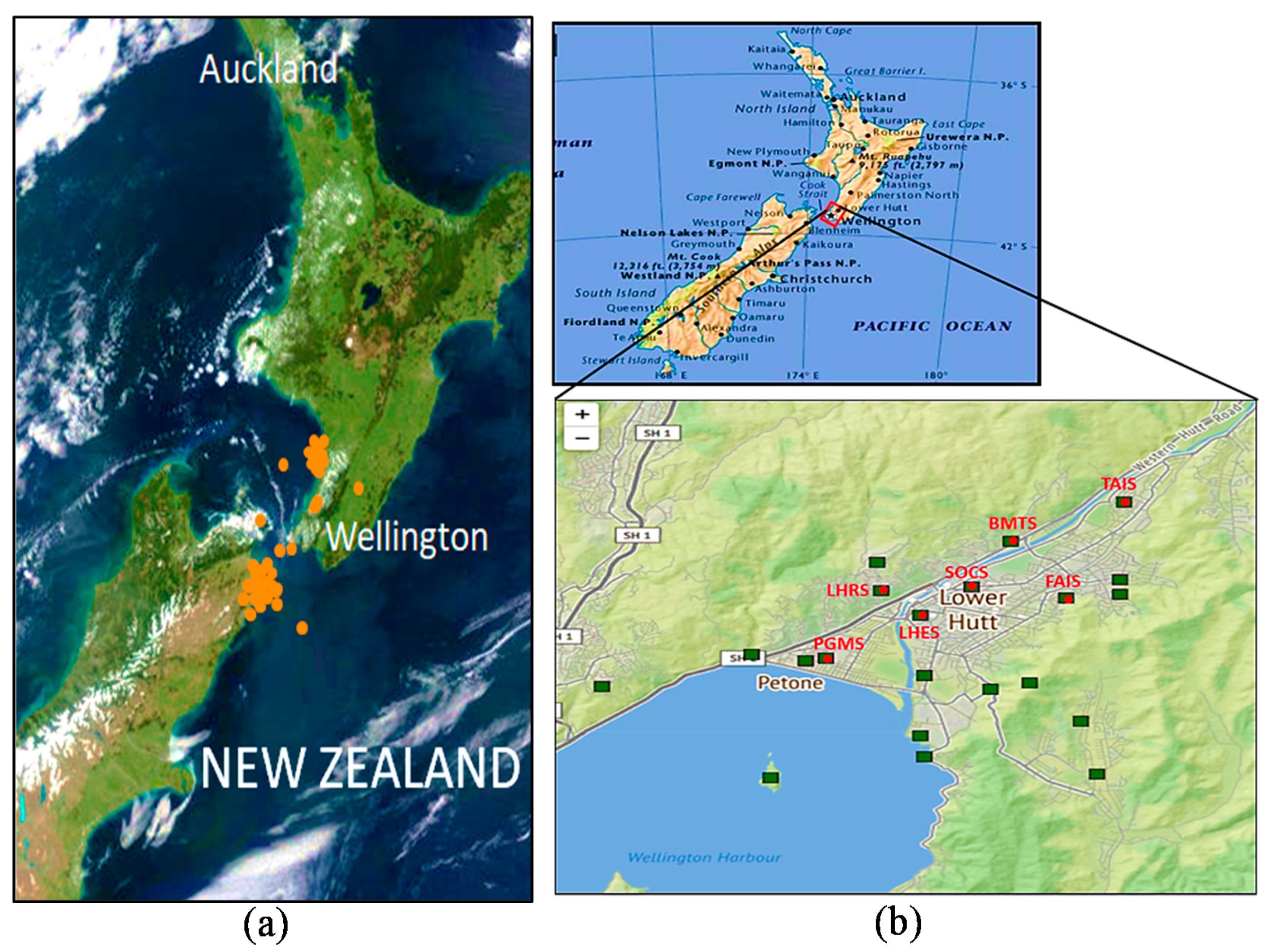
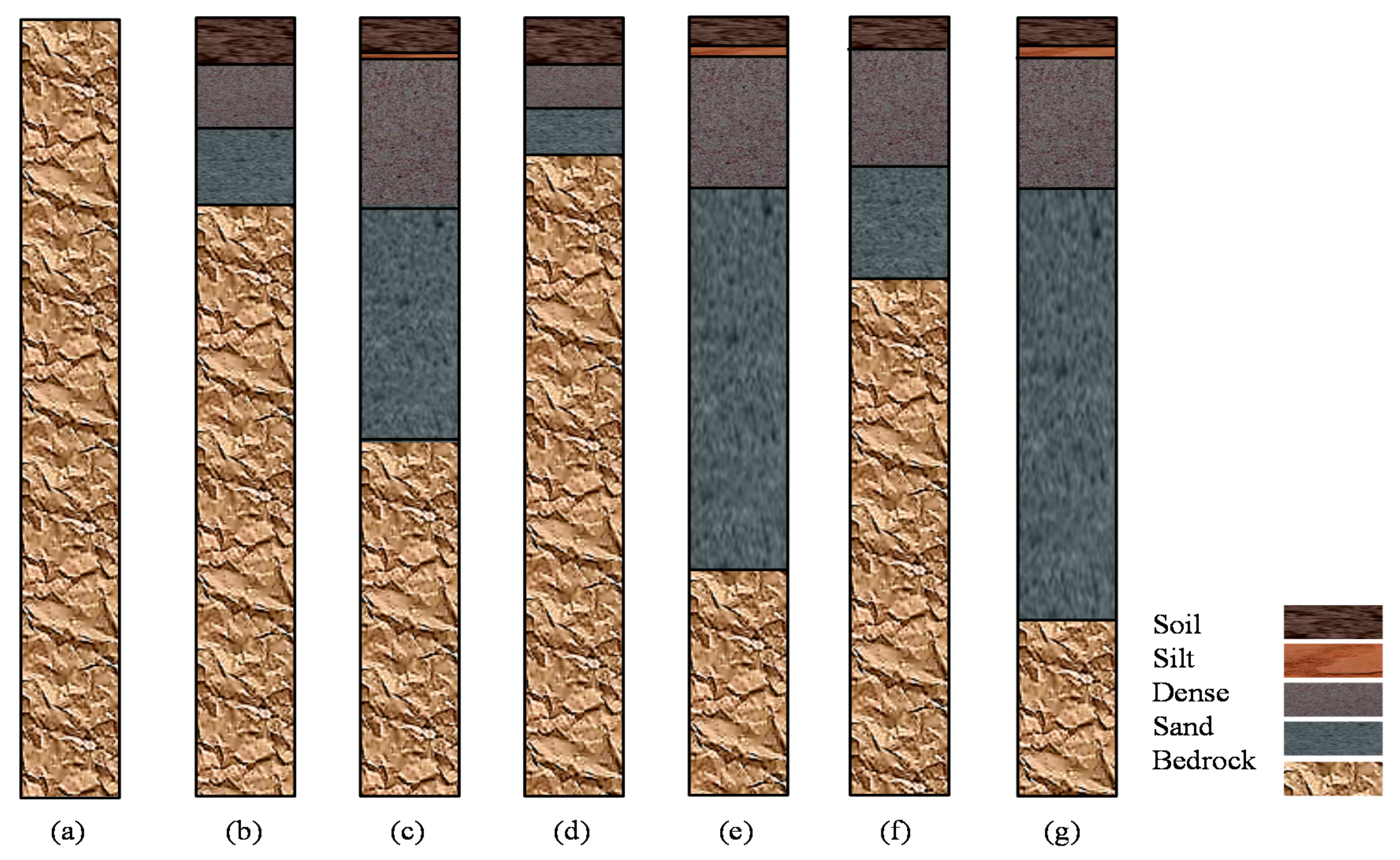
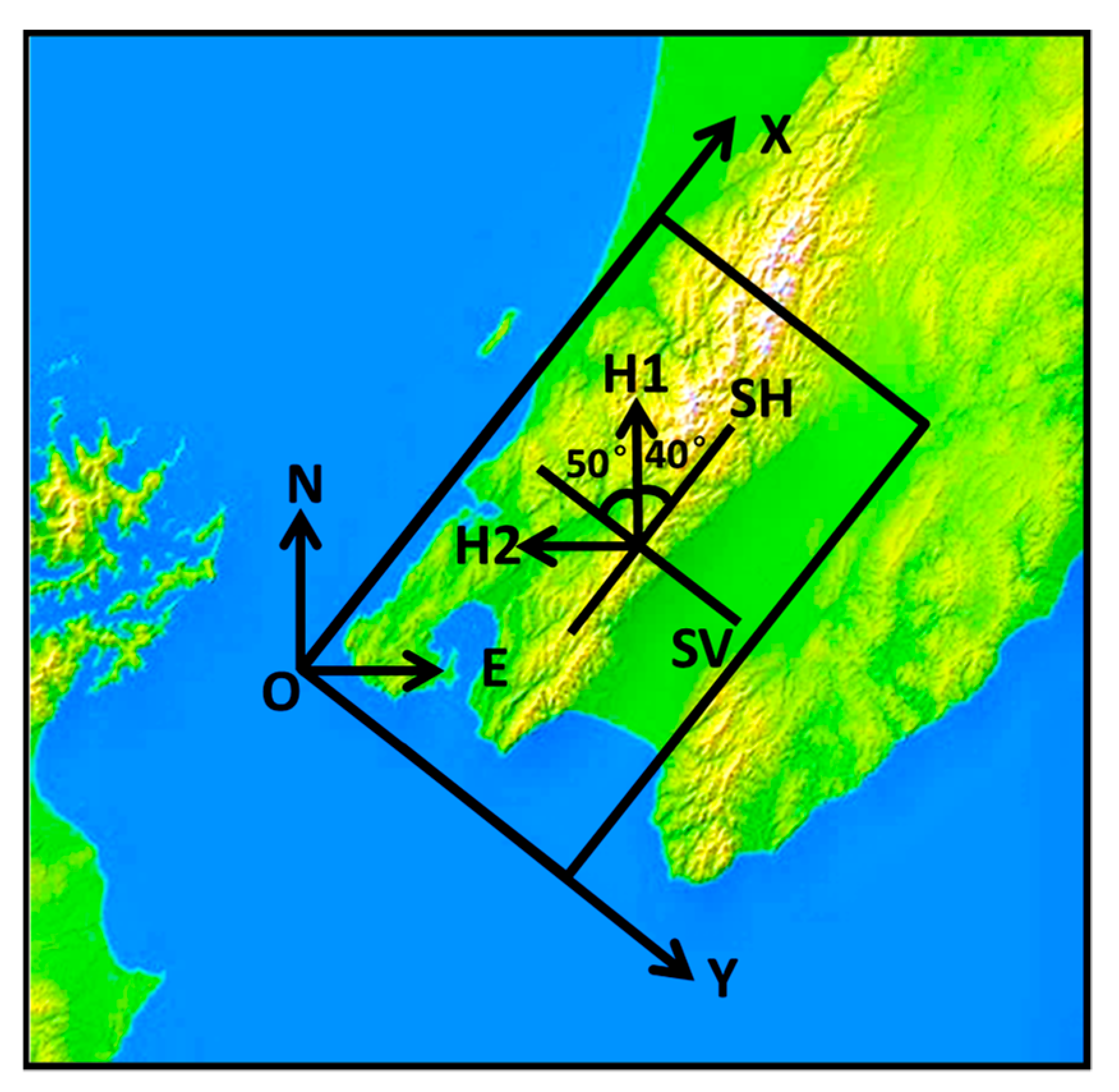
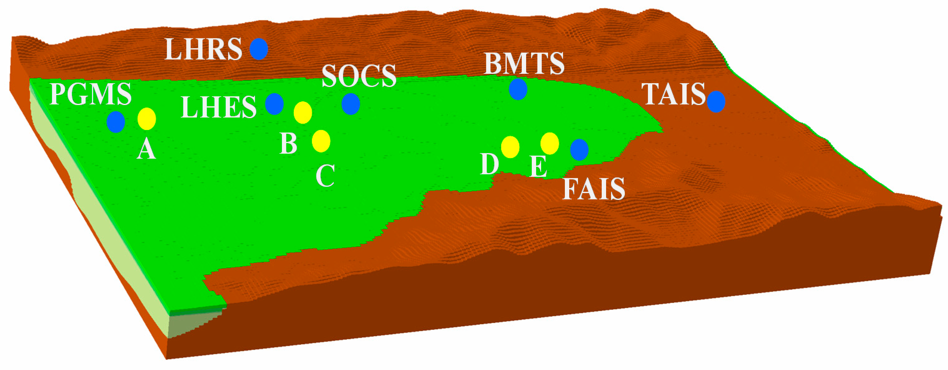
2.1. Geological Condition

The Lower Hutt Valley is a middle-sized sedimentary basin located in the Wellington Metropolitan area, New Zealand. The valley is about 10 km wide and 35 km long and is surrounded by hills in the east and the north, while it is open to Wellington Bay in the west. Figure 1a displays a location map of the valley, and a detailed map of a small zone 10 km long and 5 km wide is shown in Figure 1b.

According to the geological exploration data provided by New Zealand’s Institute of Geological and Nuclear Sciences (GNS), a local site in the Lower Hutt Valley with a length of 8400 m and a width of 5600 m was selected. There were four irregular layers of sediments over the bedrock. The S-wave velocity varied from 175 m/s to 300 m/s in the top layer, 300 m/s to 330 m/s in the second layer, 330 m/s to 500 m/s in the third layer and 500 m/s to 1500 m/s in the bottom layer. The S-wave velocity of the bedrock layer was 1500 m/s. As shown in Figure 1b, 7 accelerometers were located in the selected zone: the accelerometer stations BMTS, LHES, FAIS, TAIS, PGMS and SOCS were located in the soft soil zone and the station LHRS in the hard rock zone. The details of the soil and bedrock characteristics for the seven stations are listed in

Table 1. Station information.

Station	Latitude (S)	Longitude (E)	Thickness of Soil Layer (m)	V30 (m/s)
LHRS	41°12′17″	174°53′35″	0.000	1500.000
BMTS	41°11′29″	174°55′34″	93.330	200.830
LHES	41°12′42″	174°54′12″	217.780	215.330
FAIS	41°12′27″	174°56′24″	62.220	206.000
TAIS	41°10′35″	174°58′12″	280.000	235.000
PGMS	41°13′28″	174°52′46″	130.670	236.000
SOCS	41°12′15″	174°54′57″	311.110	240.170

. The 1-D soil layer histogram of the seven stations was extracted from the 3-D geological structure of the lower Hutt gorge, as shown in Figure 2. As the soil properties are directly related to the amplification characteristics of the surface, the first-order frequencies and the equivalent shear wave velocities of the 1-D soil layer at each station were calculated. The results are shown in Table 1.

According to the geological hazard information network of New Zealand (https://www.geonet.org.nz, accessed on: 27 June 2021), the NS and EW components of the earthquake records from the bedrock to the soil layers of the 7 stations were used, as shown in Table 1. Since each station had two horizontal components in the seismic records, the records first needed to be processed. Figure 3 shows the two horizontal components (SV and SH) at each station.

The original data of the horizontal observation records provided by the New Zealand geological disaster information network were recorded in two horizontal directions, where horizontal axis 1 was along the north direction (H1) and horizontal axis 2 along the west direction (H2). The angle between the X-direction of the Lower Hutt basin model and the geographical east-west direction was about 50°. The horizontal observation records H1 and H2 for the basin can be decomposed into SV and SH directions. The acceleration time history in the SH direction can be determined by Equation (1):

$$SH=H_{1}COS{40}^{\circ }-H_{2}COS{50}^{\circ }$$

(1)

2.2. Preparation of the Data

2.2.1. Amplification Factor

To estimate the surface amplification of the soil response with respect to the bedrock response, frequency-dependent seismic amplification factors were used to compute the soil effect of this valley surface. The standard spectral ratio [35] was used to calculate the amplification factors of the site location. This is defined as the spectral ratio of a sedimentary site with respect to a nearby bedrock reference site. A high-pass filtering program (JMTEST) method was used to smooth selected acceleration time histories, and then a fast Fourier transform (FFT) computer program was employed to obtain Fourier spectra of the acceleration time history at each soil station and bedrock station. For each earthquake, the spectral ratio of the Fourier spectra at each soil station to the spectrum at the bedrock station was used to estimate the frequency-dependent amplification factors, AFF (amplification Fourier factors) [5], from Equation (2):

$$AFF=\frac{F_{SH}^{}{}^{surface}}{F_{SH}^{}{}^{bedrock}}$$

(2)

where F_SH is the Fourier amplitude spectrum in the SH (S-wave horizon) direction at the soil surface or bedrock.

Then, for each group of acceleration time histories at soil stations, a mean frequency-dependent amplification factor was computed from the average AFF at a given frequency value [36], using Equation (3):

$$\overline{AFF}=\frac{{\displaystyle \sum _{\mathrm{i}=1}^{n}AF{F}_{\mathrm{i}}}}{\mathrm{n}}$$

(3)

2.2.2. Surface Amplification Factors at Lower Hutt Valley

The seismic response records of 44 earthquakes in the Lower Hutt Valley were selected to calculate the amplification factors for all 6 soil stations, according to Equations (1) and (2).

The amplified spectra were obtained by calculating the ratio of the acceleration records of the six stations in the soft layer vs. the bedrock station (LHRS), and parts of the results are shown in Figure 4. The amplification factors at the six stations were also obtained by calculating the average of the amplified spectrum.

Table 2. Amplification factors for earthquakes at 7 stations.

Station Magnitude	LHRS	BMTS	LHES	FAIS	TAIS	PGMS	SOCS
M4.5	1.00	1.78	2.56	1.90	3.10	1.95	3.04
M5.8	1.00	2.01	2.81	1.91	3.65	2.06	3.24
M5.1	1.00	1.61	3.42	1.81	2.98	2.06	3.27
M4.0	1.00	1.26	2.09	1.42	2.72	1.50	2.38
M4.3	1.00	—	2.78	1.93	3.06	2.20	3.33
M4.8	1.00	2.96	2.45	—	2.70	2.21	3.85
M4.5	1.00	2.77	2.08	—	2.50	1.99	2.86
M4.0	1.00	2.49	2.36	—	2.45	2.48	2.93
M4.7	1.00	1.55	2.31	2.28	3.06	2.05	2.57
M4.6	1.00	3.10	2.39	2.13	2.71	2.27	3.16
M4.3	1.00	1.86	2.76	1.91	2.87	2.45	3.42
M4.8	1.00	1.71	2.38	1.89	—	1.98	—

shows some of the average amplification factors calculated using Equation (2).

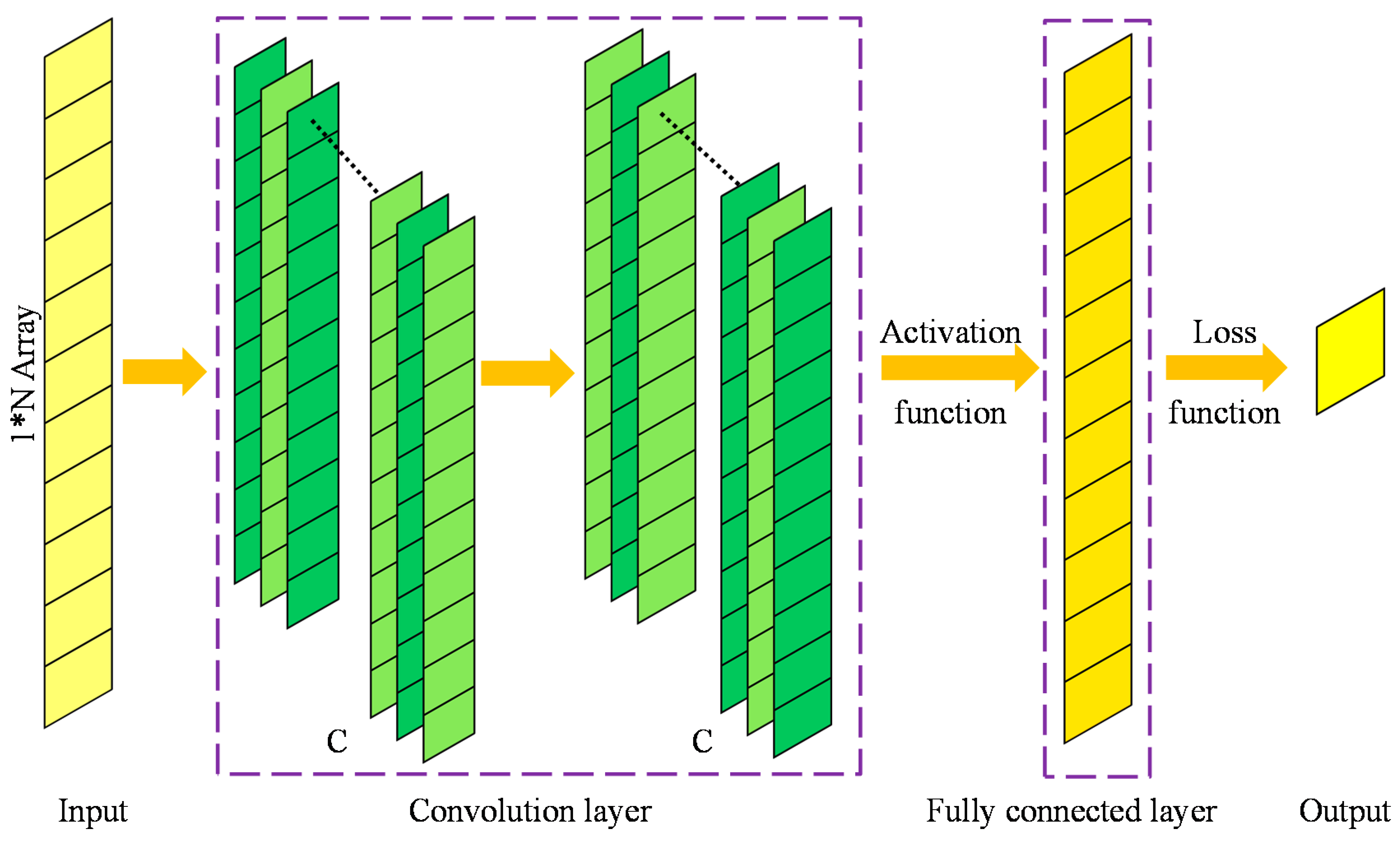
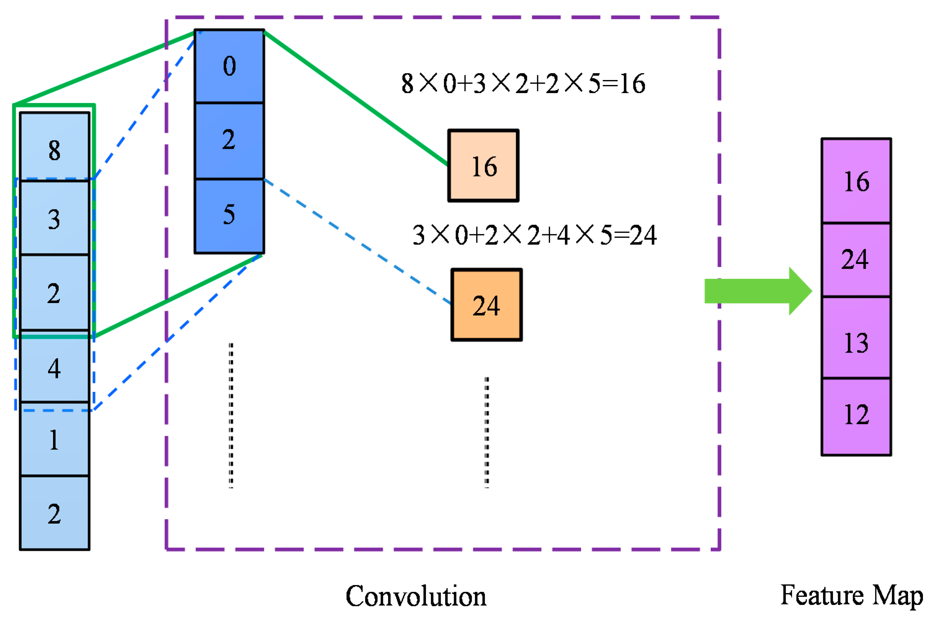
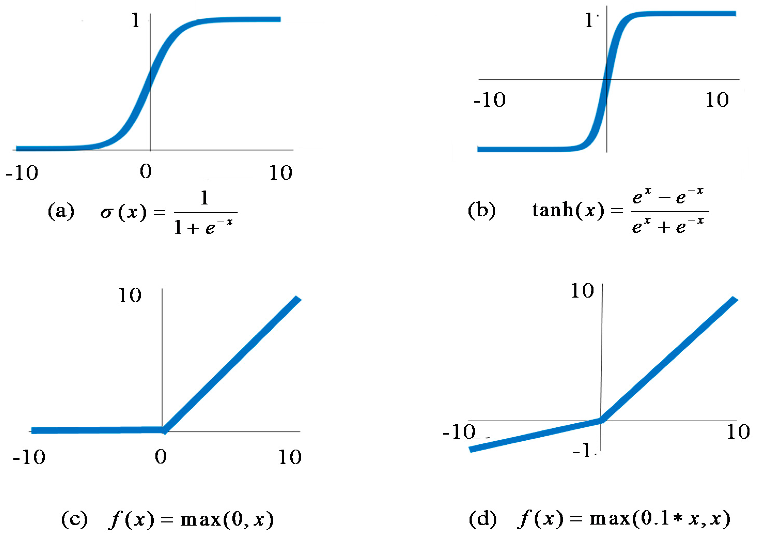
2.3. 1-D Convolutional Neural Network

As shown in Figure 5, a standard CNN model usually includes the input layers, convolution layers, a fully connected layer and an output layer. The input data were transferred through a series of layers (two convolution layers, activation function, loss function). Finally, the mapping calculation obtained the amplification factors. Specifically, the input of the 1-D CNN was either a 1 × N or an N × 1 array. As shown in Figure 5, an N × 1 array was passed through a series of convolution layers and the fully connected layer. Then, the amplification factors for the local ground motion were obtained in the output layer.

As shown in Figure 6, the convolution process was to multiply each element in the convolution kernel with the corresponding element in a sub-region (e.g., green box or blue dotted box) of the input data of the convolution layer and to sum the products to obtain an element in the feature map. Each time, the sub-region moved down by one step, and the process was repeated until all elements of the input data were involved. Finally, the convolution operation formed a new array (i.e., the feature map).

The activation function has a non-linear ability that gives the neural network better learning capabilities. Commonly used activation functions include the sigmoid, tanh, ReLU (rectified linear unit) and LeakyReLU functions, as shown in Figure 7. The LeakyReLU activation function was used in this study, as it is much faster than the sigmoid function and the tanh function.

Loss Function

The loss function was employed to evaluate the convergence of the trained CNN. It was embedded in the output layers. In this paper, the convergence of the network training process was evaluated by the validation samples. The loss function (RMSE, root mean squared error) was as given in Equation (4).

$$RMSE=\sqrt{\frac{1}{N}{\displaystyle \sum _{t=1}^N{(predicte{d}_t-label)}^2}}$$

(4)

where N is the number of validation samples.

2.4. Design of the Models

In this section, a novel method based on the CNN model was established to predict the ground motion amplification. Compared with the traditional classical regression model that can usually use only two variables for the regression task, the CNN can use multivariate regression techniques to predict the results.

2.4.1. Parameters of the Models

In this section, the CNN method was established to predict the local site amplification based on earthquake observation records. The sampling data used in the proposed CNN models involved 44 seismic events. The input data of the samples were extracted from 40 seismic incidents recorded at 7 stations (

Table 3. Design of CNN-FSPA.

	CNN-FSPA
Total	44 earthquakes (274)
Training	40 earthquakes (246)
Validation	40 earthquakes (246)
Testing	4 earthquakes (28)

). The geological exploration data of the 7 stations were provided by New Zealand’s Institute of Geological and Nuclear Sciences (GNS) and the observation records were downloaded from the New Zealand’s geohazard information network (GeoNet) (https://www.geonet.org.nz, accessed on: 27 June 2021). The output data of the samples were directly computed using Equation (2) from the downloaded observation records. A series of input variables of the proposed CNN model were specified: the station latitude, longitude, magnitude, focal depth, epicentral distance, soil layer thickness, V₃₀ (equivalent shear wave velocity at a calculated depth of 30 m in the overlying soil layer) and the observation records of the bedrock PGAr (peak ground acceleration of rock). Based on a number of the input variables and output variables of the samples, an effective and reasonable CNN model was trained, and a CNN-based prediction method was obtained. With the trained CNN model, the ground motion amplification factors of the Lower Hutt Valley could be predicted, and the amplification characteristics of this engineering site could be investigated.

A 1-D CNN structure was established using the ‘Deep Learning Toolbox’ of MATLAB (MathWorks Inc., Natick, MA, USA), including convolution layers, activation layers (leaky ReLU activation function) and one fully connected layer (FC). The convolution kernel size and layer number were adjusted according to different situations. The CNN structure was designed according to the ground motion situation considered in this study. The weights of the CNN and the internal parameters were adjusted to achieve the best local site amplification prediction effect. The data were preprocessed and then input into the CNN for network training. Part of the dataset was used for network training, and the other part was used for testing. Furthermore, padding was employed to preserve the information on the edges.

2.4.2. Description of the Models

Figure 8 shows the location map of the 7 stations (blue points) and 5 selected unrecorded location points (yellow points). The CNN models were based on the sample datasets obtained from the nearest 44 earthquake records collected from the 7 stations. Two kinds of CNN prediction models were trained, with sample parameters as shown in Table 3 and

Table 4. Design of CNN-PSPA.

	CNN-PSPA
Total	All Stations (274)	All Stations (274)	All Stations (274)	All Stations (274)	All Stations (274)	All Stations (274)
Training	Non-SOCS (237)	Non-PGMS (233)	Non-TAIS (235)	Non-FAIS (242)	Non-LHES (235)	Non-BMTS (232)
Validation	(237)	(233)	(235)	(242)	(235)	(232)
Testing (PSPA)	SOCS (37)	PGMS (41)	TAIS (39)	FAIS (32)	LHES (39)	BMTS (42)

.

(1) CNN-FSPA (full-station predicted amplification) model: in this model, 40 of the 44 earthquake records were used for training and the remaining 4 for testing the model. The detailed information of CNN-FSPA is shown in Table 3.

(2) CNN-PSPA (part-station predicted amplification) models: in these models, data from 6 of the 7 stations were used for training and the data from the other station were used for testing. A total of 6 CNN sub-models were built, namely, non-SOCS, non-PGMS, non-TAIS, non-FAIS, non-LHES and non-BMTS. The detailed information of CNN-PSPA is shown in Table 4.

In the CNN-FSPA model, the comparisons between the observed value and the predicted value were used for testing the CNN’s prediction abilities. In the CNN-PSPA models, the trained model was used to analyze the prediction error of the site amplification factors of unrecorded locations. The station data that were not included in the training samples, were used for testing the prediction abilities of the CNN-PSPA models for prediction of unrecorded locations.

3. Results and Discussion

In the following, the amplification factors of the seven stations obtained using Equation (3) were used to conduct an error analysis between the real values and predicted values of the amplification factors. The error of the amplification factor is defined in Equation (5).

$$error=\frac{\left|predicted-observed\right|}{observed}\times 100\%$$

(5)

3.1. Comparisons with BPNN Models

The CNN models were trained for predicting the site amplification factors of the Lower Hutt Valley. To demonstrate the advantages of the CNN models in predicting the site amplification factors, traditional BPNN models were also trained on similar data for comparison. These models were named BPNN-FSPA and BPNN-PSPA.

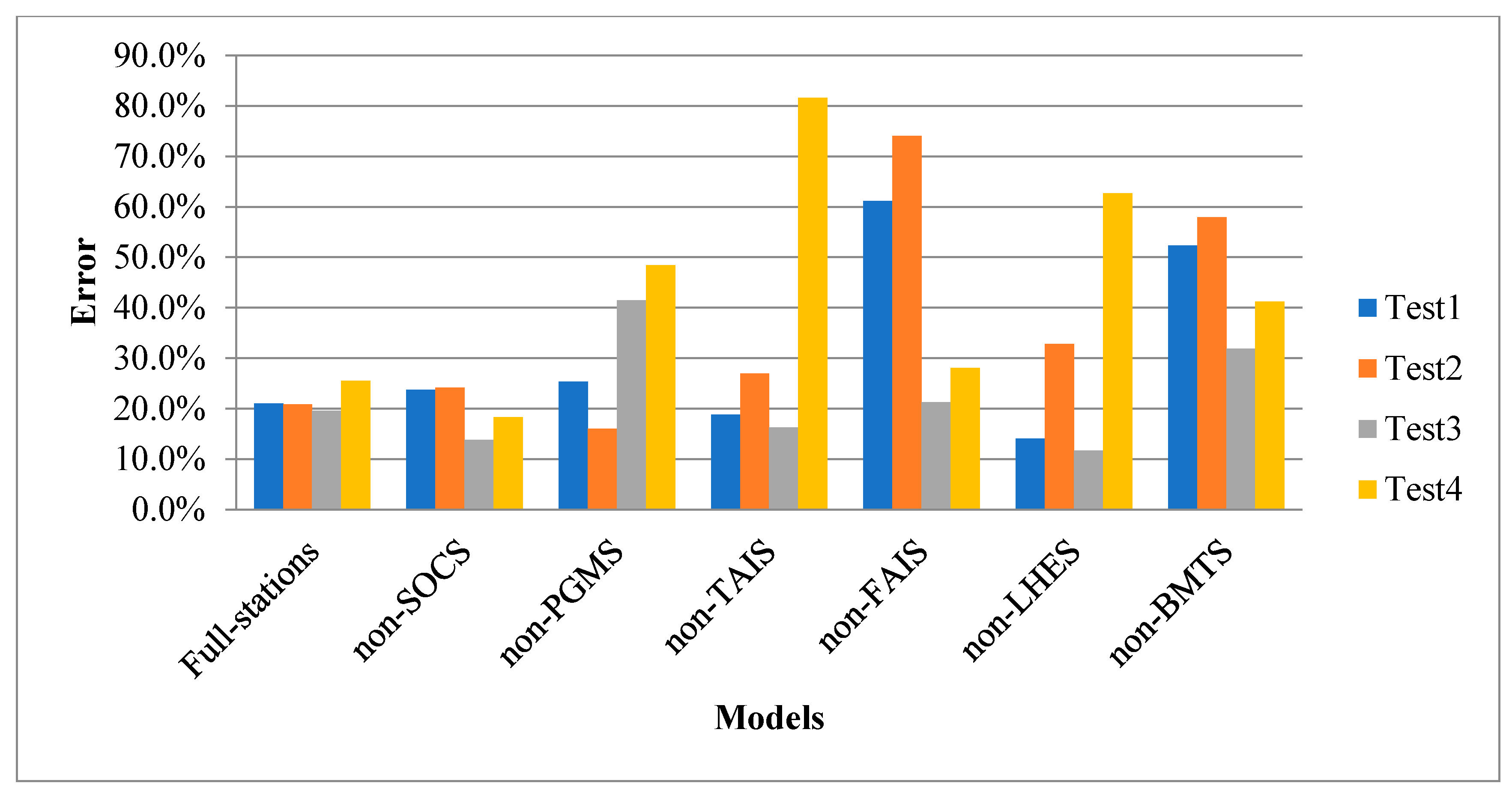
3.1.1. Effect of Parameters on Different Models

First, the differences between the CNN and BPNN models were considered for studying the effect of the parameters. The four groups of training parameters for the CNN and BPNN models are listed in

Table 5. Four tests with different parameters.

Models	CNN		BPNN
	Kernel Size	Kernel Number	Hidden Layer Size
Test 1	[2 1] [3 1]	190 310	5
Test 2	[2 1] [3 1]	190 320	6
Test 3	[2 1] [3 1]	198 320	7
Test 4	[2 1] [3 1] [4 1]	190 320 322	8

. In the BPNN models, the tests referred to different hidden layers, as shown in Table 5. The errors of the prediction results are shown in Figure 9 for the CNN models and Figure 10 for the BPNN models.

Figure 9 shows that with different model parameters, the prediction results for the CNN models did not differ much, and the training effect was relatively stable. In contrast, the BPNN training results appeared to be quite variable for all the tests and were extremely unstable with respect to the different model parameters, as shown in Figure 10. Figure 10 also shows that Test 1 had the worst testing results and the highest error rate. Furthermore, the variability of the red histogram was the largest, showing that Test 2 was the most unstable. Test 3 was relatively stable and its error rate was the lowest. Furthermore, in the non-FAIS model, the training effect was encouraging, except in Test 1. Among the four tests, the most stable BPNN model was the non-SOCS model.

As shown from the analyses of the CNN models and BPNN models, the parameters could be further optimized for the two kinds of models. Compared to the BPNN models, the CNN models had better accuracy and stability with different model parameters. To ensure the accuracy and stability of the prediction results, the BPNN should avoid the Test 1 parameters with a high error rate and the Test 2 parameters with poor stability.

3.1.2. Comparisons of Prediction Results

From Figure 9 and Figure 10, the worst and the best CNN and BPNN models, respectively, were selected for comparison. The best CNN model, except for CNN-FSPA, was the non-FAIS model with Test 2 parameters and the best BPNN model, except for BPNN-FSPA, was the non-LHES model with Test 3 parameters. The worst CNN model was the non-BMTS model with Test 4 parameters and the worst BPNN model was the non-TAIS model with Test 4 parameters. The prediction results and errors for four earthquakes (M4.5, M5.6, M5.1 and M4.0) at four stations (FAIS, LHES, BMTS and TAIS) are shown in

Table 6. Comparisons of CNNs and BPNNs.

Model	Magnitude	CNN-PSPA			BPNN-PSPA
		Observed (FAIS)	Predicted (FAIS)	Error	Observed (LHES)	Predicted (LHES)	Error
Best testing	M4.5	2.86	2.48	13.2%	2.05	2.51	18.3%
	M5.6	1.89	1.98	4.7%	2.55	2.69	5.2%
	M5.1	1.90	1.93	1.7%	2.80	3.04	8.3%
	M4.0	1.81	2.12	17.3%	3.42	2.53	26.0%
Model	Magnitude	Observed (BMTS)	Predicted (BMTS)	Error	Observed (TAIS)	Predicted (TAIS)	Error
Worst testing	M4.5	2.79	1.99	28.6%	2.34	3.85	64.4%
	M5.6	2.45	2.30	6.1%	3.56	7.30	104.8%
	M5.1	1.78	1.77	0.7%	3.10	4.61	48.6%
	M4.0	2.01	1.81	9.9%	3.65	5.33	45.9%

.

As shown in Table 6, all the errors of the CNN models were lower than those of the corresponding BPNN models for the same earthquakes. In addition, the worst testing model (non-BMTS) of the CNNs had an error rate of 25.0% and the corresponding non-TAIS model of the BPNNs had an error rate of 81.6%.

It can also be seen from Table 6 that the error difference between the best and the worst predictions of the CNNs was much lower than for the BPNNs. Comparisons between the best and worst of the CNN-PSPA models showed that the errors of the results did not differ much. Furthermore, the earthquakes with magnitude 5.1 gave the best results, with little fluctuation in this CNN-PSPA. The CNNs showed better stability and less sensitivity to the parameters. In contrast, the difference between the best and worst tests of the BPNNs was significant. The worst of the BPNNs showed both a larger variance and the largest error of 104.8%, appearing in the M5.6 earthquakes. The BPNN-PSPA test for a magnitude of 5.6 showed the difference between the worst test with the largest error rate of 104.8% and the best test with the smallest error rate of 5.2%. It can be seen that the BPNN models were very unstable and were adversely affected by changing the parameters. The CNN models outperformed the corresponding BPNN models in terms of test stability.

Both the stability and the accuracy analyses showed that the CNNs were significantly better than the BPNNs.

3.2. Prediction Results of the CNN-FSPA Model

As the last section stated, the CNN models showed better prediction ability for the site amplification factors than the traditional BPNN models. In the following two sections, the CNN-FSPA and CNN-PSPA models are discussed in detail with regard to parameter optimization and prediction results. Based on the optimized parameters, the comparatively better prediction model was trained for predicting the site amplification factors of the Lower Hutt Valley.

3.2.1. Testing of Different Parameters

The CNN-FSPA model was trained using 40 earthquakes for training and 4 earthquakes for testing. The average test errors of the CNN-FSPA model for different CNN parameters are listed in

Table 7. No padding and padding of the CNN models.

No Padding			Padding
Kernel Size	Kernel Number	Error	Kernel Size	Kernel Number	Error
[2 1]	192	18.3%	[2 1]	192	19.7%
[2 1] [3 1]	190 320	13.0%	[2 1] [3 1]	190 320	12.6%
[2 1] [3 1] [4 1]	190 320 330	13.3%	[2 1] [3 1] [4 1]	190 320 330	12.8%

.

Table 7 shows that by varying the models with and without padding, it was found that the models with more than one convolutional layer showed lower error rates and better predictions than their counterparts without padding. The prediction results of the CNNs with different convolutional layers and convolutional kernels are also listed in Table 7. For the CNNs with one convolutional layer, the errors of the test results were 18.3–19.7%. For the CNNs with two convolutional layers, the error rate was 12.6–13.0%. For the CNNs with three convolutional layers, the error rate was slightly higher at 12.8–13.3%. Overall, the testing error could be reduced by about 1% using the padding function of the CNN models with two or three convolutional layers.

The test with the lowest error was selected to give the training parameters for determining the CNN structure. The specific structural parameters of the CNNs are shown in

Table 8. Structural parameters of the 1-D CNNs.

Layer	Type	Kernel No.	Kernel Size	Stride	Padding	Activation
1	Input	None	None	None	None	None
2	Convolution (C1)	190	2 × 1	1	1	Leaky ReLU
3	Convolution (C2)	320	3 × 1	1	1	Leaky ReLU
4	FC	None	None	None	None	None
5	Output	None	None	None	None	None

. There were five layers with two convolutional layers in this test. In the first convolutional layer, 190 convolutional kernels with a size of 2 × 1 were used to process the input data. In the second convolutional layer, the number of convolutional kernels was 320 with a size of 3 × 1.

Selection of the appropriate parameters according to the actual data had a significant effect on the training of the CNN model.

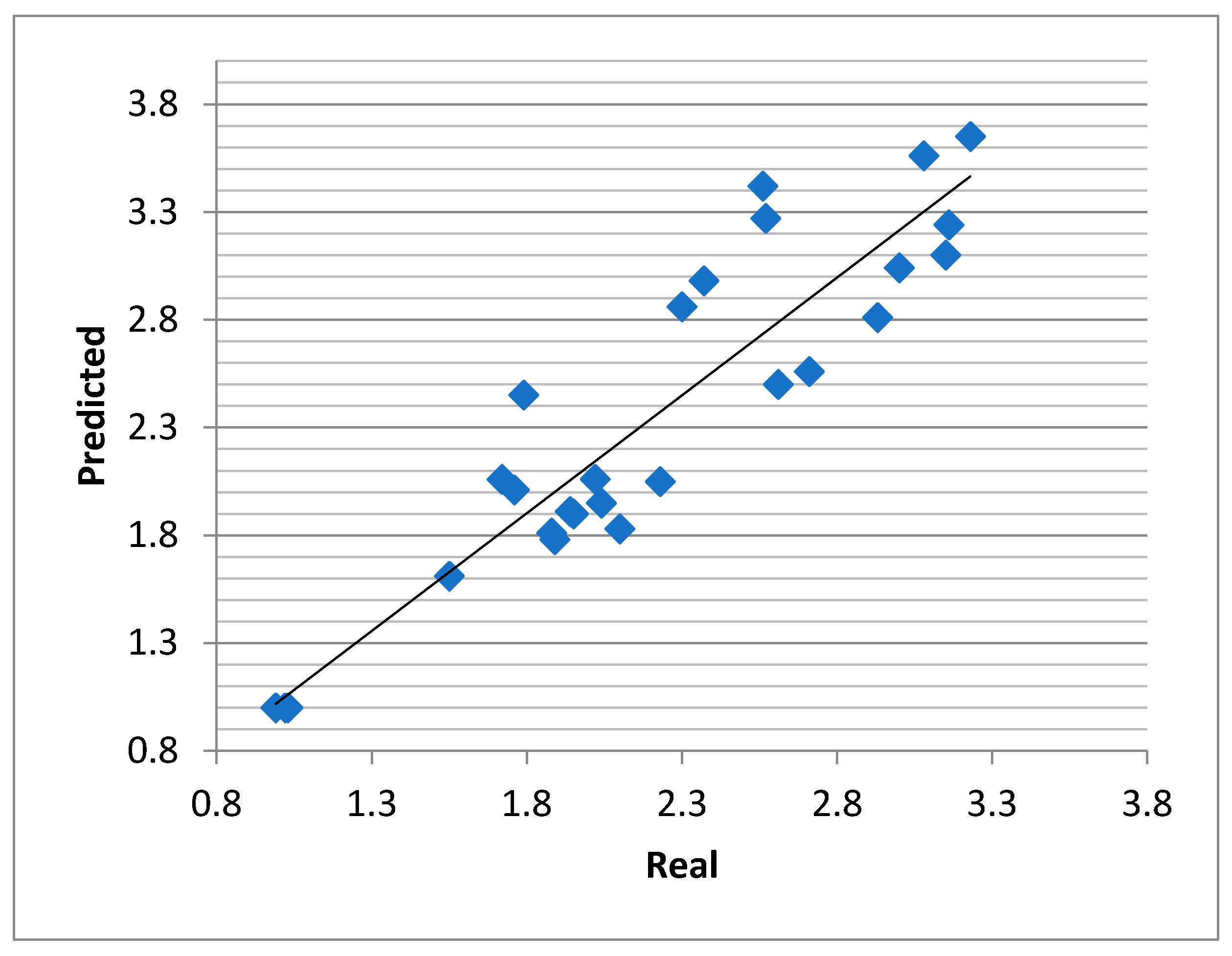
3.2.2. Comparisons with Recorded Results

With the two convolutional layers shown in Table 8, the CNN-FSPA model gave better prediction results than the other models with different parameters. Therefore, the selected CNN-FSPA model was used to predict the amplification factors of the seven known station locations. The prediction results for earthquakes with magnitudes of 4.0, 4.5, 5.1 and 5.6 are listed in

Table 9. Prediction results for the CNN-FPSA.

Station	Earthquakes	Observed	Predicted	Error	Average Error
LHRS	M4.5	1.00	1.02	2.0%	8.5%
	M5.6	1.00	0.99	1.0%
	M5.1	1.00	1.02	2.0%
	M4.0	1.00	1.03	2.9%
BMTS	M4.5	2.45	1.79	26.9%
	M5.6	1.78	1.89	5.8%
	M5.1	2.01	1.76	12.4%
	M4.0	1.61	1.55	3.7%
LHES	M4.5	2.05	2.23	8.1%
	M5.6	2.56	2.69	5.1%
	M5.1	2.81	2.93	4.1%
	M4.0	3.42	2.66	22.2%
FAIS	M4.5	2.86	2.30	19.6%
	M5.6	1.90	1.95	2.6%
	M5.1	1.91	1.94	1.5%
	M4.0	1.81	1.88	3.7%
TAIS	M4.5	3.56	3.08	13.5%
	M5.6	3.10	3.15	1.6%
	M5.1	3.65	3.23	11.5%
	M4.0	2.98	2.37	20.5%
PGMS	M4.5	1.83	2.10	12.9%
	M5.6	1.95	2.04	4.4%
	M5.1	2.06	2.02	1.9%
	M4.0	2.06	1.72	16.5%
SOCS	M4.5	2.50	2.61	4.2%
	M5.6	3.04	3.00	1.3%
	M5.1	3.24	3.16	2.5%
	M4.0	3.27	2.57	21.4%

. The comparisons of the predicted and observed results are also shown in Table 9 and Figure 11.

Table 9 shows that the total average prediction error was 8.5%, which is relatively low. In addition, it can clearly be seen from Table 9 that most of the prediction errors for small earthquakes such as M4.0 and M4.5 were rather high, probably due to the effect of anomalous amplification of seismic waves by the soil layer. In contrast, the predictions of the middle-sized earthquakes such as M5.1 and M5.6 were better. Furthermore, it can be observed that the stations FAIS, PGMS and SOCS (but not the bedrock station LHES) had low prediction errors. This indicates that the CNN-FSPA model had good testing results for those three stations.

As shown in the Figure 11, the scatter points were evenly and regularly distributed around the black oblique line. This shows that this model was able to provide a good prediction.

3.3. Prediction Results of CNN-PSPA Models

The CNN-PSPA models were also trained for predicting the site amplification factors of the Lower Hutt Valley. The CNN-PSPA models included six sub-models, described in Section 2.4.2. Unlike the trained CNN-FSPA model, which included the information for the testing samples, the trained CNN-PSPA models did not include the information for the testing samples. Since there was no information for test location at all in the training samples, the errors of the prediction results at test locations could be regarded as similar to those for the other unrecorded locations used for the reliability analysis of this type of model. In the following, the six CNN-PSPA models are used to discuss their prediction ability via error analysis. The errors of the amplification factors were also computed using Equation (4).

3.3.1. Optimal Parameters for CNN-PSPA Models

Since the accuracy and the stability in the training of the CNN models were mainly dependent on the parameters of the convolutional layers and convolutional kernels, error values computed with different parameters were used to optimize the CNN-PSPA models. In order to construct a more optimal CNN-based model, four groups with different convolutional kernel sizes and kernel numbers were selected for evaluating the prediction errors. The average errors of the six CNN-PSPA models with different parameters are shown in

Table 10. Results for CNN-PSPA with different parameters.

Models	Predicted Station	Kernel Size	Kernel Number	Ave. Error	Error Fluctuation
non-SOCS	SOCS	[2 1] [3 1]	190 310	16.5%	8.7%
		[2 1] [3 1]	190 315	18.5%
		[2 1] [3 1]	190 318	14.2%
		[2 1] [3 1]	190 320	22.9%
non-PGMS	PGMS	[2 1] [3 1]	190 320	23.1%	9.1%
		[2 1] [3 1]	196 310	19.0%
		[2 1] [3 1]	196 320	24.5%
		[2 1] [3 1]	198 320	15.4%
non-TAIS	TAIS	[2 1] [3 1] [4 1]	190 320 322	16.5%	4.3%
		[2 1] [3 1] [4 1]	190 320 325	18.6%
		[2 1] [3 1] [4 1]	190 320 330	17.9%
		[2 1] [3 1] [4 1]	192 320 330	20.8%
non-FAIS	FAIS	[2 1] [3 1]	190 315	22.4%	9.8%
		[2 1] [3 1]	190 320	12.6%
		[2 1] [3 1]	196 320	13.2%
		[2 1] [3 1]	190 326	17.9%
non-LHES	LHES	[2 1] [3 1]	188 320	22.1%	9.9%
		[2 1] [3 1]	190 320	12.2%
		[2 1] [3 1]	192 320	16.0%
		[2 1] [3 1]	196 320	21.6%
non-BMTS	BMTS	[2 1] [3 1]	190 320	21.1%	3.9%
		[2 1] [3 1]	192 320	22.4%
		[2 1] [3 1]	192 330	25.0%
		[2 1] [3 1]	196 320	23.6%

. The differences in the average error between the maximum and minimum for each CNN-PSPA model are also listed in Table 10.

Table 10 shows that the average error values varied with the different parameters for all of the six CNN-PSPA models. The error differences of the six models ranged from 14.3%, 15.5%, 17.9%, 12.6%, 12.6%, and 21.2% to 23.0%, 24.5%, 23.9%, 22.5%, 22.1%, and 25.0%. Regarding the errors of the six models, the maximum change was 9.9% in the non-LHES model, and the minimum change was 3.9% in the non-BMTS model.

The non-BMTS model was the least sensitive to the CNN parameters, while the non-LHES model was the most influenced by the parameters. From Table 10, the optimal values of the six models were extracted from the four group parameters for subsequent predictions. Among the six CNN-PSPA models, the best prediction model was the non-LHES model, which had a relative error of 12.2%. The model with the biggest error of all the six models was the non-BMTS model, which had an average error of 21.1%. The accuracy and stability of the trained CNN-PSPA models remained at a reasonable level for different network parameters.

Table 10 shows that the sensitivity of the test results was inversely proportional to the error rate of the results. For example, the non-LHES model had the highest error fluctuation among the six CNN-PSPA models when trained with different parameters, but it had the lowest error value among the models. Compared to the five other models, it was more sensitive to the parameters within the control range. However, the models with higher errors did not fluctuate as much. This led to stable prediction results by the CNN-PSPA model, even with different training parameters.

3.3.2. Comparisons with Observed Results

The non-LHES model, with the best test results among all the six CNN-PSPA models, was selected for predicting all the site amplification factors of 39 earthquakes at the LHES station location, where five earthquake records were not included. The prediction results for the 39 earthquakes are listed in

Table 11. Prediction results for non-LHES.

Number	Earthquake	Epicentral Distance (km)	Depth (km)	CNN-PSPA			Average Error
				Observed (LHES)	Predicted (LHES)	Error
1	M4.0	104	40	3.42	2.51	26.5%	12.7%	12.2%
2	M4.0	86	31	2.18	2.41	10.6%
3	M4.1	113	11	3.03	2.38	21.5%
4	M4.1	84	10	2.78	2.50	10.1%
5	M4.1	57	12	3.04	2.45	19.4%
6	M4.1	42	12	2.36	2.49	5.5%
7	M4.2	113	6	3.83	2.70	29.5%
8	M4.2	15	26	2.32	2.60	12.1%
9	M4.3	72	11	2.73	2.45	10.3%
10	M4.3	79	16	2.09	2.23	6.7%
11	M4.3	85	32	2.39	2.28	4.6%
12	M4.4	98	10	2.60	2.51	3.5%
13	M4.4	76	5	2.71	2.50	7.7%
14	M4.4	87	28	2.47	2.28	7.7%
15	M4.5	16	24	2.67	2.30	13.9%
16	M4.5	106	36	2.05	2.39	16.5%
17	M4.5	85	30	2.45	2.30	6.1%
18	M4.5	79	7	3.20	2.55	20.3%
19	M4.5	86	30	2.55	2.31	9.4%
20	M4.6	116	32	2.31	2.42	4.8%	11.7%
21	M4.6	82	12	3.31	2.63	20.5%
22	M4.7	81	33	2.36	2.21	6.4%
23	M4.7	57	13	3.23	2.59	19.8%
24	M4.8	72	11	2.59	2.39	7.7%
25	M4.8	74	12	2.78	2.39	14.0%
26	M4.8	84	54	2.76	2.59	6.2%
27	M4.8	74	9	2.91	2.42	16.8%
28	M5.0	86	36	2.63	2.34	11.0%
29	M5.0	50	13	2.73	2.28	16.5%
30	M5.0	76	8	2.99	2.43	18.7%
31	M5.1	78	5	2.81	2.52	10.4%
32	M5.2	121	8	2.90	2.66	8.3%
33	M5.4	82	34	2.14	2.24	4.7%
34	M5.5	74	17	2.38	2.15	9.7%
35	M5.5	91	15	3.65	2.97	18.6%
36	M5.6	85	7	2.56	2.42	5.5%
37	M5.6	82	13	2.58	2.38	7.8%
38	M5.8	85	37	2.11	2.48	17.5%
39	M6.2	104	34	2.57	2.81	9.3%

. The site amplification factors obtained from the observation records are listed in Table 11 for comparison. By comparing with the corresponding observation results, the errors were also calculated for all the incidents, as shown in Table 11.

Table 11 shows that the total average prediction error was 12.2%, which was relatively low. In addition, it can clearly be seen from Table 11 that most of the prediction errors for small earthquakes such as M4.0 and M4.5 were rather high, probably due to the effect of anomalous amplification of seismic waves by the soil layer. In contrast, the predictions for the medium-sized earthquakes such M5.1 and M5.6 were better. Furthermore, low prediction errors for stations FAIS, PGMS and SOCS (but not the bedrock station LHES) were observed. This indicates that the CNN-FSPA model showed good training for those three stations. Compared with the CNN-FSPA model in Table 9, the average error of the CNN-PSPA model was slightly higher by 3.7%.

In addition, the errors for small earthquakes with large epicenter and source depths, such as earthquakes with serial numbers 1, 3, 7 and 16, were significantly higher than those for other earthquakes. However, for medium earthquakes with large epicentral distances and focal depths, such as earthquakes with serial numbers 20, 32 and 39, errors were lower and predictions were satisfactory.

3.3.3. Comparison with CNN-FSPA Model

To estimate the ability of CNN-PSPA prediction models, all the six trained models (non-SOCS, non-PGMS, non-TAIS, non-FAIS, non-BMTS and non-LHES) were used to predict the site amplification factors at the corresponding stations. For example, the trained non-SOCS model predicted the site amplification factor at the SOCS station. The test-sample data were selected using the four earthquakes that were also used to test the CNN-FSPA model. All error values for the site amplification factors at the six soil stations were calculated from the six trained CNN-PSPA models. The corresponding errors for the same four earthquakes at the six station locations based on the trained CNN-FSPA models were also predicted for comparisons. All the errors of the predicted values for these seven CNN models are listed in

Table 12. Errors for CNN-FSPA and CNN-PSPA.

Magnitude	Predicted	CNN-PSPA		CNN-FSPA
		Models	Error	Error
M4.5	SOCS	non-SOCS	21.7%	4.2%
	PGMS	non-PGMS	29.9%	12.9%
	TAIS	non-TAIS	37.9%	13.5%
	FAIS	non-FAIS	16.8%	19.6%
	BMTS	non-BMTS	12.1%	26.9%
	LHES	non-LHES	16.5%	8.1%
M5.6	SOCS	non-SOCS	16.6%	1.3%
	PGMS	non-PGMS	21.7%	4.4%
	TAIS	non-TAIS	1.8%	1.6%
	FAIS	non-FAIS	4.7%	2.6%
	BMTS	non-BMTS	21.0%	5.8%
	LHES	non-LHES	5.5%	5.1%
M5.1	SOCS	non-SOCS	10.2%	2.5%
	PGMS	non-PGMS	16.5%	1.9%
	TAIS	non-TAIS	13.5%	11.5%
	FAIS	non-FAIS	1.7%	1.5%
	BMTS	non-BMTS	20.8%	12.4%
	LHES	non-LHES	10.4%	4.1%
M4.0	SOCS	non-SOCS	10.0%	21.4%
	PGMS	non-PGMS	21.3%	16.5%
	TAIS	non-TAIS	12.7%	20.5%
	FAIS	non-FAIS	17.3%	3.7%
	BMTS	non-BMTS	12.2%	3.7%
	LHES	non-LHES	26.5%	22.2%

.

Table 12 shows that since the prediction errors of the CNN-FSPA model were lower than those of the CNN-PSPA model, the CNN-FSPA model was significantly better than the CNN-PSPA model. This phenomenon shows that the more station data that are included in the CNN training, the better the CNN model is trained. The included test information could influence the accuracy and credibility of the prediction results. Table 12 also shows that although the trained CNN-PSPA model had higher errors than the trained CNN-FSPA model in any prediction, it had relatively smaller differences, demonstrating that reliable amplification factors could be obtained even using the trained CNN-PSPA model.

Table 12 also shows that, as for the predictive regularities of the CNN-FSPA models, the CNN-PSPA predictions for the medium-sized earthquakes such as M5.1 and M5.6 were better than those for micro-earthquakes such as M4.0 and M4.5. The non-FAIS model showed outstanding predictive power for medium earthquakes, even though it exhibited a relatively high error for the micro-earthquakes such as M4.0 and M4.5. In contrast, for the CNN-FSPA model, it should be noted that the non-FAIS and non-BMTS models for M4.5 and the non-TAIS model for M4.0 unexpectedly exhibited higher error rates than the CNN-PSPA model.

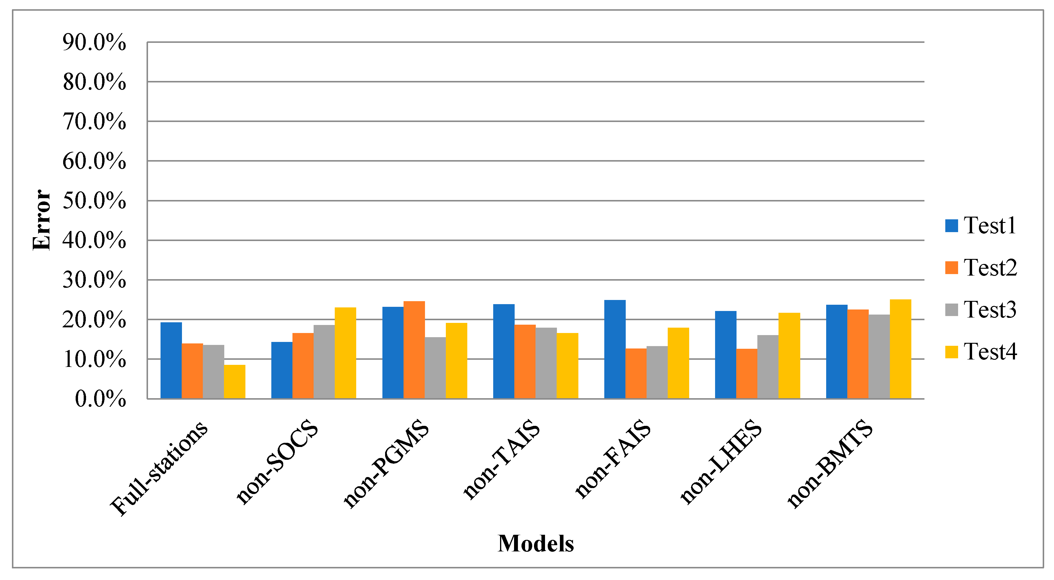
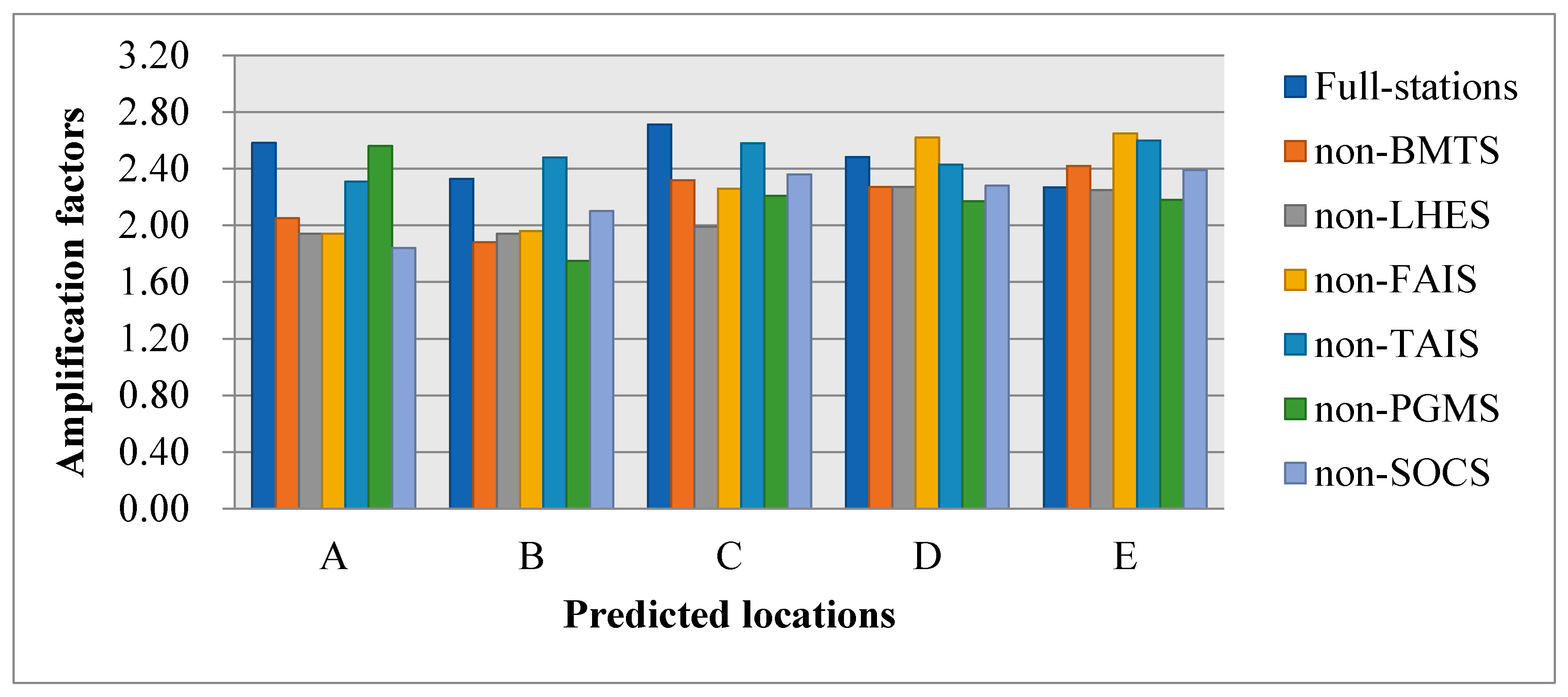
3.4. Comparisons of Unrecorded Locations

To predict the amplification characteristics of unrecorded locations, five randomly selected site points, other than those shown in Figure 8, named A, B, C, D and E, were used to predict their amplification factors. With the earthquakes with magnitude M5.0 as an example, the seven trained CNN models with the best testing results, namely, CNN-FSPA, non-SOCS, non-PGMS, non-TAIS, non-FAIS, non-BMTS and non-LHES, were used to calculate the amplification factors of the five points. The prediction results of the amplification factors at these five unrecorded points by the seven CNN-models are shown in Figure 12.

Figure 12 shows that the amplification factors varied in the order E > D > C > A > B. As shown in Figure 12, all the five points, A, B, C, D and E, exhibited a large amplification factor when the CNN-FSPA model was used for prediction. If only the CNN-PSPA model (which showed better training) was used for prediction, the prediction results of the non-FAIS and non-LHES models for the five points were similar.

However, the predicted amplification factor using the CNN-PSPA model was still rather small compared to that of the CNN-FSPA model. The reason for this was its insufficient training quantity and incomplete learning. Therefore, the task of predicting the amplification factor of unknown points should be performed in a series of steps. These inspiring results could provide a reference for seismic intensity setting in practical projects.

For discussing the differences in the prediction results, the relative error of two types of CNNs was used, as given by Equation (6):

$$Erro{r}_{PSPA}=\frac{\left|Valu{e}_{\mathrm{CNN}-\mathrm{PSPA}}-Valu{e}_{\mathrm{CNN}-\mathrm{FSPA}}\right|}{\left|Valu{e}_{\mathrm{CNN}-\mathrm{FSPA}}\right|}\times 100\%$$

(6)

where $Erro{r}_{PSPA}$ denotes the difference rate between the CNN-PSPA and the CNN-PSPA, and $Valu{e}_{\mathrm{CNN}-\mathrm{PSPA}}$ and $Valu{e}_{\mathrm{CNN}-\mathrm{FSPA}}$ are the predicted amplification factors of the CNN-PSPA model and CNN-FSPA model, respectively. The error values of the predicted amplification factors of CNN-PSPA for the five points (A, B, C, D and E) for an earthquake with M5.0 are shown in

Table 13. Relative errors of CNN-PSPA.

	Models	CNN-PSPA
Points		Non- SOCS	Non- PGMS	Non- TAIS	Non- FAIS	Non- LHES	Non- BMTS
A		26.8%	8.6%	10.5%	24.9%	24.9%	20.6%
B		9.8%	24.8%	6.1%	15.8%	16.7%	19.3%
C		13.0%	18.5%	4.9%	16.7%	26.6%	14.5%
D		8.2%	12.6%	2.2%	5.2%	8.6%	8.6%
E		5.0%	3.9%	12.7%	14.4%	0.9%	6.2%

.

Compared with the CNN-FSPA model, the CNN-PSPA models clearly showed a high error rate at point A, indicating that more attention is required. In addition, for the predictions in Table 13, it can be seen that the amplification factors of points D and E showed good predictions and small fluctuations in each model. Therefore, the CNN-FSPA model could predict the amplification factor of an unrecorded location well.

4. Conclusions

In this paper, a 1-D CNN method was used to predict the ground motion amplification of the Lower Hutt Valley. Based on a relatively small sample dataset, two kinds of CNN models were established and applied, to predict the amplification factors of the local zone. The prediction results were inspiring.

Based on the above results, the following conclusions were drawn.

Compared with BNPP models, the trained CNN models were influenced little by different training parameters, leading to a more stable trained model.

The CNN-FSPA model could effectively predict the station amplification factors from the existing data; the accuracy was 91.5%, which was 15.8% higher than that of the corresponding BPNN-FSPA model.

Both CNN-FSPA and CNN-PSPA models could effectively predict the amplification factors of local ground motion.

The comparisons of the CNN-FSPA and CNN-PSPA models showed that, by increasing the number of earthquakes and the training samples, a prediction model of the ground surface amplification could be established based on strong earthquake observations.

5. Discussion

(1) For the data processing, we used the Fourier transform method, and also tried other data processing methods such as the wavelet transform method, to find more accurate data processing methods for subsequent research.

(2) Since it is difficult for numerical simulations to contain all the seismic information, in this study we used a combination of seismic records and CNN to predict the amplification factors with an increased quantity of seismic data. In the future, we will also use a combination of simulations and observed data to improve the prediction accuracy via migration learning.

(3) The current trend is to use deep learning to solve some prediction problems. With the construction of regional station networks and the increase in training samples, we will continue to collect seismic information from other sites, such as Ashighara Valley and Ohba Valley in Japan, the Volvi basin in Greece and so on. Therefore, using machine learning to predict earthquakes has good prospects for development.

References

1. Sánchez-Sesma, F.; Crouse, C.B. Effects of site geology on seismic ground motion: Early history. Earthq. Eng. Struct. Dyn. 2015, 44, 1099–1113. [Google Scholar] [CrossRef]
2. Trifunac, M.D. Site conditions and earthquake ground motion–A review. Soil Dyn. Earthq. Eng. 2016, 90, 88–100. [Google Scholar] [CrossRef]
3. Markham, C.S.; Bray, J.D.; Macedo, J.; Luque, R. Evaluating nonlinear effective stress site response analyses using records from the Canterbury earthquake sequence. Soil Dyn. Earthq. Eng. 2016, 82, 84–98. [Google Scholar] [CrossRef] [Green Version]
4. Harmsen, S.C. Determination of site amplification in the Los Angeles urban area from inversion of strong-motion records. Bull. Seismol. Soc. Am. 1997, 87, 866–887. [Google Scholar]
5. Hartzell, S. Variability in nonlinear sediment response during the 1994 Northridge, California, earthquake. Bull. Seismol. Soc. Am. 1998, 88, 1426–1437. [Google Scholar]
6. Kaveh, A.; Bakhshpoori, T.; Hamzeh-Ziabari, S.M. Derivation of New Equations for Prediction of Principal Ground-Motion Parameters using M5’ Algorithm. J. Earthq. Eng. 2016, 20, 910–930. [Google Scholar] [CrossRef]
7. Pezzo, E.D.; Martino, S.D.; Parrinello, M.T.; Sabbarese, C. Seismic site amplification factors in Campi Flegrei, Southern Italy. Phys. Earth Planet. Inter. 1993, 78, 105–117. [Google Scholar] [CrossRef]
8. Sandikkaya, M.A.; Akkar, S.; Bard, P.Y. A Nonlinear Site-Amplification Model for the Next Pan-European Ground-Motion Prediction Equations. Bull. Seismol. Soc. Am. 2013, 103, 19–32. [Google Scholar] [CrossRef]
9. Yu, J. The Choice of Reference Sites for Seismic Ground Amplification Analyses: Case Study at Parkway, New Zealand. Bull. Seismol. Soc. Am. 2003, 93, 713–723. [Google Scholar] [CrossRef]
10. Zaslavsky, Y.; Shapira, A. Experimental study of topographic amplification using the Israel Seismic Network. J. Earthq. Eng. 2000, 4, 43–65. [Google Scholar] [CrossRef]
11. Ferrari, R.D.; Ferretti, G.; Barani, S.; Pepe, G.; Cevasco, A. On the role of stiff soil deposits on seismic ground shaking in western Liguria, Italy: Evidences from past earthquakes and site response. Eng. Geol. 2017, 226, 172–183. [Google Scholar] [CrossRef]
12. Kanai, K.; Tanaka, T. On Microtremors. VIII. Bull. Earthq. Res. Inst. 1961, 39, 97–114. [Google Scholar]
13. Nakamura, Y.A. Method for Dynamic Characteristics Estimation of Subsurface Using Microtremor on Ground Surface. Q. Rep. Rtri. 1989, 30, 25–33. [Google Scholar]
14. Sadiq, M.T.; Yu, X.; Yuan, Z.; Fan, Z.; Rehman, A.U.; Li, G.; Xiao, G. Motor imagery EEG signals classification based on mode amplitude and frequency components using empirical wavelet transform. IEEE Access 2019, 7, 127678–127692. [Google Scholar] [CrossRef]
15. Sadiq, M.T.; Yu, X.; Yuan, Z.; Aziz, M.Z. Motor imagery BCI classification based on novel two-dimensional modelling in empirical wavelet transform. Electron. Lett. 2020, 56, 1367–1369. [Google Scholar] [CrossRef]
16. Sadiq, M.T.; Yu, X.; Yuan, Z.; Zeming, F.; Rehman, A.U.; Ullah, I.; Li, G.; Xiao, G. Motor imagery EEG signals decoding by multivariate empirical wavelet transform-based framework for robust brain–computer interfaces. IEEE Access 2019, 7, 171431–171451. [Google Scholar] [CrossRef]
17. Bernal, D. Amplification factors for inelastic dynamic p–Δ effects in earthquake analysis. Earthq. Eng. Struct. Dyn. 1987, 15, 635–651. [Google Scholar] [CrossRef]
18. Tropeano, G.; Soccodato, F.M.; Silvestri, F. Re-evaluation of code-specified stratigraphic amplification factors based on Italian experimental records and numerical seismic response analyses. Soil Dyn. Earthq. Eng. 2018, 110, 262–275. [Google Scholar] [CrossRef]
19. Glinsky, N.; Bertrand, E.; Régnier, J. Numerical simulation of topographical and geological site effects. Applications to canonical topographies and Rognes hill, South East France. Soil Dyn. Earthq. Eng. 2019, 116, 620–636. [Google Scholar] [CrossRef]
20. Kamai, R.; Abrahamson, N.A.; Silva, W.J. Nonlinear Horizontal Site Amplification for Constraining the NGA-West2 GMPEs. Earthq. Spectra 2014, 30, 1223–1240. [Google Scholar] [CrossRef]
21. Athanasopoulos, G.A.; Pelekis, P.C.; Leonidou, E.A. Effects of surface topography on seismic ground response in the Egion (Greece) 15 June 1995 earthquake. Soil Dyn. Earthq. Eng. 1999, 18, 135–149. [Google Scholar] [CrossRef]
22. Riga, E.; Makra, K.; Pitilakis, K. Aggravation factors for seismic response of sedimentary basins: A code-oriented parametric study. Soil Dyn. Earthq. Eng. 2016, 91, 116–132. [Google Scholar] [CrossRef]
23. Wald, D.J.; Graves, R.W. The seismic response of the Los Angeles basin, California. Bull. Seism. Soc. Am. 1998, 88, 337–356. [Google Scholar]
24. Khanbabazadeh, H.; Iyisan, R.; Ansal, A.; Hasal, M.E. 2D non-linear seismic response of the Dinar basin, TURKEY. Soil Dyn. Earthq. Eng. 2016, 89, 5–11. [Google Scholar] [CrossRef]
25. Stamati, O.; Klimis, N.; Lazaridis, T. Evidence of complex site effects and soil non-linearity numerically estimated by 2D vs 1D seismic response analyses in the city of Xanthi. Soil Dyn. Earthq. Eng. 2016, 87, 101–115. [Google Scholar] [CrossRef]
26. Semblat, J.F.; Duval, A.M.; Dangla, P. Numerical analysis of seismic wave amplification in Nice (France) and comparisons with experiments. Soil Dyn. Earthq. Eng. 2000, 19, 347–362. [Google Scholar] [CrossRef] [Green Version]
27. Meza-Fajardo, K.C.; Varone, C.; Lenti, L.; Martino, S.; Semblat, J.F. Surface wave quantification in a highly heterogeneous alluvial basin: Case study of the Fosso di Vallerano valley, Rome, Italy. Soil Dyn. Earthq. Eng. 2019, 120, 292–300. [Google Scholar] [CrossRef]
28. Abdullah, S.M. On linear site amplification behavior of crustal and subduction interface earthquakes in Japan: (1) regional effects, (2) best proxy selection. Bull. Earthq. Eng. 2018, 17, 119–139. [Google Scholar]
29. Kim, S.; Hwang, Y.; Seo, H.; Kim, B. Ground motion amplification models for Japan using machine learning techniques. Soil Dyn. Earthq. Eng. 2020, 132, 106095. [Google Scholar] [CrossRef]
30. Yuen, K.V.; Ortiz, G.A.; Huang, K. Novel nonparametric modeling of seismic attenuation and directivity relationship. Comput. Methods Appl. Mech. Eng. 2016, 311, 537–555. [Google Scholar] [CrossRef]
31. Güllü, H.; Erçelebi, E. A neural network approach for attenuation relationships: An application using strong ground motion data from Turkey. Eng. Geol. 2007, 93, 65–81. [Google Scholar] [CrossRef]
32. Yaghmaei-Sabegh, S.; Rupakhety, R. A new method of seismic site classification using HVSR curves: A case study of the 12 November 2017 Mw 7.3 Ezgeleh earthquake in Iran. Eng. Geol. 2020, 270, 105574. [Google Scholar] [CrossRef]
33. Yaghmaei-Sabegh, S.; Tsang, H.-H. A new site classification approach based on neural networks. Soil Dyn. Earthq. Eng. 2011, 31, 974–981. [Google Scholar] [CrossRef]
34. Mu, H.Q.; Yuen, K.V. Ground Motion Prediction Equation Development by Heterogeneous Bayesian Learning. Comput. Civ. Infrastruct. Eng. 2016, 116, 761–776. [Google Scholar] [CrossRef]
35. Sadiq, M.T.; Yu, X.; Yuan, Z. Exploiting dimensionality reduction and neural network techniques for the development of expert brain–computer interfaces. Expert Syst. Appl. 2021, 164, 114031. [Google Scholar] [CrossRef]
36. Hough, S.E.; Altidor, J.R.; Anglade, D.; Given, D.; Yong, A. Localized damage caused by topographic amplification during the 2010 M7.0 Haiti earthquake. Nat. Geosci. 2010, 3, 778–782. [Google Scholar] [CrossRef]
Figure 1. Location maps. (a) Locations of earthquake focuses; (b) station locations in Lower Hutt basin in New Zealand.
Applsci 11 11650 g001
Figure 2. Borehole records. (a) LHRS; (b) BMTS; (c) LHES; (d) FAIS; (e) TAIS; (f) PGMS; (g) SOCS.
Applsci 11 11650 g002
Figure 3. Seismic records from the Lower Hutt basin in New Zealand.
Applsci 11 11650 g003
Figure 4. Sediment-to-rock Fourier spectral ratios (FSRs) of stations.
Applsci 11 11650 g004
Figure 5. One-dimensional CNN model for predicting site amplification factors.
Applsci 11 11650 g005
Figure 6. Based on comparisons of the three activation functions, the ReLU activation function was used in our model as it was much faster than the sigmoid and tanh functions.
Applsci 11 11650 g006
Figure 7. Activation function: (a) sigmoid; (b) tanh; (c) ReLU; (d) LeakyReLU.
Applsci 11 11650 g007
Figure 8. Location map.
Applsci 11 11650 g008
Figure 9. Errors of CNN predictions.
Applsci 11 11650 g009
Figure 10. Errors of BPNN predictions.
Applsci 11 11650 g010
Figure 11. Comparison of predicted and observed results.
Applsci 11 11650 g011
Figure 12. Prediction of the amplification factors of unrecorded points by seven models.
Applsci 11 11650 g012