Functional Effects of Permeability on Oldroyd-B Fluid under Magnetization: A Comparison of Slipping and Non-Slipping Solutions

Abstract

In this article, the impact of Newtonian heating in addition to slip effects was critically examined on the unsteady magnetohydrodynamic (MHD) flow of an Oldroyd-B fluid near an infinitely vertical plate. The functional effects such as the retardation and relaxation of materials can be estimated for magnetized permeability based on the relative decrease or increase during magnetization. From this perspective, a new mathematical model was formulated based on non-slippage and slippage postulates for the Oldroyd-B fluid with magnetized permeability. The heat transfer induction was also examined through a non-fractional developed mathematical model for the Oldroyd-B fluid. The exact solution expressions for non-dimensional equations of velocity and temperature were explored by employing Laplace integral transformation under slipping boundary conditions under Newtonian heating. The heat transfer rate was estimated through physical interpretation by considering the limits on the solutions induced by the Nusselt number. To comprehensively discuss the dynamics of the considered problem, the physical impacts of different parameters were studied and reverberations were graphically highlighted and deliberated. Furthermore, in order to validate the results, two limiting models, namely the Maxwell model and the second grade model, were used to compare the relevant flow characteristics. Additionally, in order to perform the parametric analysis, the graphical representation was portrayed for non-slipping and slipping solutions for velocity and temperature.

1. Introduction

For a variety of fluids such as polymer solutions, certain oils, toothpaste, clay and melts, as well as blood, the specific elastic and viscous features are simultaneously those of non-Newtonian fluids. A wide range of scientists and researchers are fascinated due to its invaluable characteristics and a wide application in modern technologies and different fields of life. Non-Newtonian fluids generally differ in the three categories: namely those of rate, differential and integral types. Substantially, the precise apprehension is that all the characteristics of such fluids cannot be expressed through one unique model; this is impossible because non-Newtonian fluids have a shear rate and shear stress that are non-linearly associated with each other. The ordinary Navier–Stokes equation cannot express the different rheological features and dynamics of such fluids, e.g., their retardation, stress differences, Weissenberg effects, relaxation, elongation, micro-structure, shear thickening/thinning, memory effects, re-coil, and yield stress. To conveniently handle the involved nonlinear additional term and to anticipate the rheological characteristics of non-Newtonian fluids, a large variety of different models have been proposed such as Jeffery’s model [1], the Maxwell model [2], the Burgers’ viscoelastic model [3], second grade fluid model [4], Sisko’s model [5] and the Oldroyd-B model [6]. In recent years, the Oldroyd-B fluid, among the many rate types of fluids, has gained a unique status because the classical Newtonian fluid and the Maxwell fluid are special cases of the Oldroyd-B fluid. The Oldroyd-B model exhibits the relaxation and retardation mechanisms and it is a very simple model which appropriately expresses the elastic and viscous behaviors of the fluid because the Oldroyd-B fluid has potential which also includes the flow history. The velocity field and stress field for the Oldroyd-B fluid were analytically examined for a constantly moving plate by Fetecau et al. [7]. Fetecau et al. [8] also extended the same investigation to explore transient channel transport for the Oldroyd-B model which settled due to the instinctive motions of the plate. Gul et al. [9] investigated the thin film motion for the transient MHD Oldroyd-B model over an oscillating belt. Tiwana et al. [10] studied the influence of ramped boundary velocity, ramped wall heating and a permeable medium on the convective transport of transient MHD Oldroyd-B fluid. Recently, the Littlewood-Paley theory was used by Wan [11] to scrutinize the universal well-posed particularities of Oldroyed-B fluid two-dimensional flow under initial conditions. The transient motion of the Oldroyd-B fluid with the existence of influential cohesion forces and its flow induced by the translational movement of the surface were inspected by Shakeel et al. [12]. Tahir et al. [13] investigated the solution in series form to inspect the fractional behavior of an Oldroyd-B fluid flow for two revolving cylinders. The same investigation was extended by Wang et al. [14], who applied an integral transform method to express the derived results’ modified Bessel function. Elhanafy et al. [15] used the numerical solution of the Oldroyd-B model to determine the blood’s movement across the abdominal aortic section. The finite difference method was applied inside a straight cloture with expanding boundaries to manipulate the heat transfer and MHD motion in an Oldroyd-B model by Ali et al. [16]. It is well-accepted fact that heat transfer from a high to low temperature wall occurs through the certain movement of a fluid—such a mechanism is called “heat convection” (advection). This is of great importance as fluid motion occurs on the basis of natural or forced convection [17,18,19,20,21,22]. Solangi et al. [23] discussed the heat transfer characteristics of large concentrations. The key point highlighted in this work is that the heat and mass behavior of the fluid are controlled by the particle’s size. Shafiq et al. [24] conducted a stimulating study for MHD convective flow with the parametric analysis of the proposed problem for thermophoretic, Blackian motion, buoyancy forces, Newtonian heating and magnetic field for concentration and temperature. Two solutions which have numerical stability were used to examine the dual results of the governing partial differential equation investigated by Hamid et al. [25]. Abdelmalek et al. [26] used the control volume finite element scheme, also known as hybrid technique, for the curved circular shape heater in addition to nanoparticles for heat transmission. The thermo-diffusion effects on the time-dependent free convective fluid flow of applying surface modification technology were determined by Kashif [27]. Further relevant studies regarding heat and mass have been studied in detail by: heat transfer approaches via analytical [28,29,30,31,32,33,34,35], numerical [36,37,38,39,40,41], with the application of fractional operators [42,43,44,45] and multi-dimensional [46,47,48,49,50,51] types.

To effectively study the dynamics of fluid flow problems, the no-slip and slip conditions were generally assumed at the boundary. In the case of the no-slip conditions, it is supposed that there is no relative movement of the fluid at the boundary, i.e., the fluid and the boundary are stationary and the speed of the flow is zero. Physically, between the surface of the fluid and the boundary, the adherence phenomenon is more dominant than the cohesive phenomenon. The no-slip condition has great applications in different practical use, regardless of a few coupled compulsions, because the complexity of flow dynamics are reduced in the case of no-slip conditions. However, some smooth surfaces exist where cohesion forces show dominance and in this case, a relative movement in the fluid was observed before the fluid moved from the boundary. For such a type of surfaces, accurate results in the case of no-slip conditions cannot produce fluid flow properties. For example, the analysis of blood transportation through arteries cannot be studied using no-slip conditions [52]. Navier presented a new technique to effectively handle such problems by using slip conditions [53]. The slip condition is strongly applicable in different areas of daily life, for example, industrial lubricants, soil degradation by erosion, medical fields—especially cleaning the artificial heart valves, by applying protrusion, different biological fluids and various type of nanofluids in porous media [54]. Related investigations on the subject of slip conditions are discussed in [55].

The objective of this study was to analyze the impact of Newtonian heating in addition to slip effects by critically examining the unsteady MHD flow of an Oldroyd-B fluid near an infinitely vertical plate. Furthermore, the functional effects such as the retardation and relaxation of materials can be estimated for magnetized permeability based on relative decrease or increase during magnetization. Exact solution expressions for non-dimensional equations of velocity and temperature were explored by employing Laplace integral transformation under slipping boundary conditions under Newtonian heating. Moreover, the heat transfer rate was estimated through physical interpretation by considering the limits on the solutions induced by the Nusselt number. The physical impacts of different parameters were studied and the reverberations were graphically highlighted and deliberated. Furthermore, two limiting models, namely the Maxwell model and second grade model, were used to compare the relevant flow characteristics in order to validate the results. Finally, in order to perform the parametric analysis, the graphical representation was portrayed for non-slipping and slipping solutions for velocity and temperature.

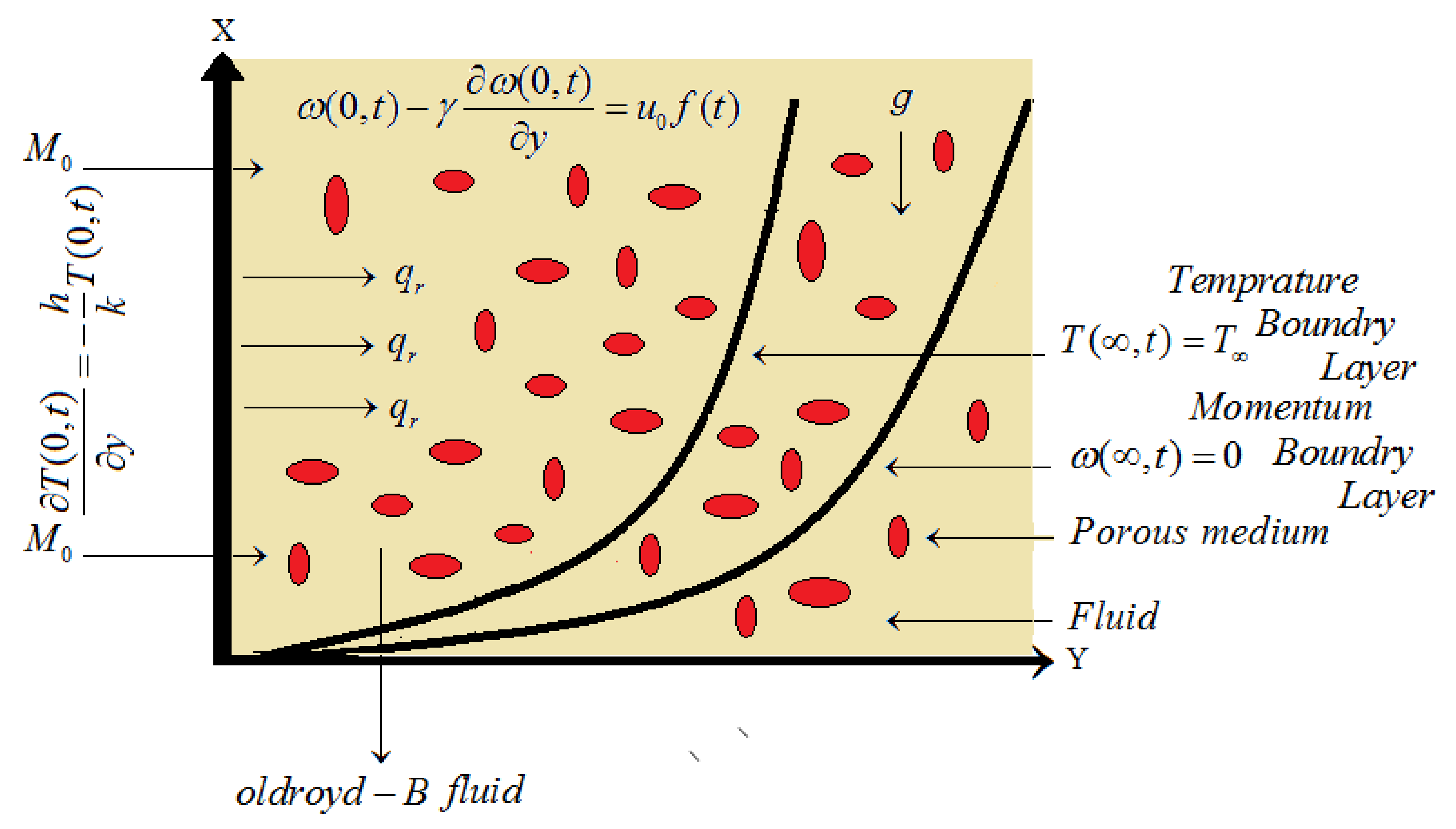
2. Mathematical Model

Consider the unsteady magnetohydrodynamic (MHD) flow of an Oldroyd-B fluid near an infinitely long plate with heat transfer under Newtonian heating. Suppose that the external magnetic forces act along the normal direction of the movement of the fluid and that the fluid is also electrically conducted. The impact of the thermal radiation is parallel to the plate but is assumed to be insignificant—the opposite is true in the horizontal direction. Velocity is considered at any point that does not only depend upon the radial distance in the proposed problem but also on the horizontal direction, i.e., the x distance. Thus, the flow in this problem is a two-dimensional flow. First of all, it is presumed that a system with no movement is a system under rest conditions. After a short interval of time, the fluid starts to move due to mixed convection, and the fluid flows along the plate as illustrated in Figure 1.

The configured flow equations for an Oldroyd-B fluid model are given by [56,57]

$$\begin{array}{c}\hfill \nabla .V=\mathbf{0},\end{array}$$

(1)

$$\begin{array}{c}\hfill \nabla .T+\rho g+J\times M=\rho \left[(V.\nabla )V+\frac{\partial V}{\partial t}\right].\end{array}$$

(2)

where $V$, $J$, $T$, $M$, $\rho$, $\rho g$ and t are the parameters used in the above equations to denote the velocity field, electric density, Cauchy stress tensor, total magnetic field (having both induced and imposed forces), fluid density, body force and time, respectively. The relation between the Cauchy stress and extra stress tensor is represented by $T$ and $S$, respectively, for the Oldroyd-B fluid formulated as

$$\begin{array}{cc}\hfill S& =pI+T,\hfill \end{array}$$

(3)

$$\begin{array}{cc}\hfill \left(S+{\lambda }_{\mathbf{1}}\frac{\partial S}{\partial t}\right)& =\mu \left(1+{\lambda }_2\frac{\partial }{\partial t}\right)A_{\mathbf{1}},\hfill \end{array}$$

(4)

$$\begin{array}{cc}\hfill A_{\mathbf{1}}& ={\left(\nabla V\right)}^T+(\nabla V),\hfill \end{array}$$

(5)

where ${\lambda }_1$, p, $I$, $\mu$, ${\lambda }_2$, $-pI$,$\frac{D}{Dt}$ and $A_{\mathbf{1}}$ denote the relaxation time, pressure, identity tensor, dynamic viscosity, retardation time, tensor’s indeterminate part, convective time derivative and Rivlin–Ericksen tensor, respectively. Furthermore, the Maxwell equations for the electric and magnetic fields are written in the following form:

$$\begin{array}{c}\hfill \Delta .M=0,\Delta \times E=-\frac{\partial M}{\partial t},\Delta \times M={\mu }_{m}J,J\times M=-\sigma M_{\mathbf{0}}^{\mathbf{2}}V.\end{array}$$

(6)

where $J$ represents the electric field, $M$ is denotes the magnetic field, $\sigma$ represents the fluid’s electrical conductivity and ${\mu }_m$ denotes the magnetic permeability. Furthermore, $M=M_0+M_1$, in which $M_0$ and $M_1$ denote the imposed and induced magnetic fields, but the induced magnetic field is not considered herein. In the present work, the velocity field is considered in the following form:

$$\begin{array}{c}\hfill V=V(y,t)=w(y,t)\mathit{i}andS=S(y,t).\end{array}$$

(7)

where $\mathit{i}$ and w represent the unit vector in the x direction and the x component of velocity $V$, respectively. By substituting Equations (3)–(7) into Equation (2) and after simplification via the application of the Rosseland approximation and Boussinesq’s approximation, we obtained the principal governing equation for the MHD Oldroyd-B fluid in addition to the initial/boundary conditions which are given as [58,59]

$$\begin{array}{cc}\hfill \left(1+{\lambda }_1\frac{\partial }{\partial t}\right)\frac{\partial w(y,t)}{\partial t}& =\upsilon \left(1+{\lambda }_2\frac{\partial }{\partial t}\right)\frac{{\partial }^{2}w(y,t)}{\partial y^2}+g\beta \left(1+{\lambda }_1\frac{\partial }{\partial t}\right)\left(T(y,t)-T_{\infty }\right)\hfill \\ & -\left(1+{\lambda }_1\frac{\partial }{\partial t}\right)\frac{\sigma M_0^2}{\rho }w(y,t),\hfill \end{array}$$

(8)

$$\begin{array}{c}\hfill C_p\frac{\partial T(y,t)}{\partial t}=\frac{k}{\rho }\frac{{\partial }^{2}T(y,t)}{\partial y^2},\end{array}$$

(9)

$$\begin{array}{c}\hfill \left(1+{\lambda }_1\frac{\partial }{\partial t}\right)S=\mu \frac{\partial w(y,t)}{\partial y},\end{array}$$

(10)

with the initial and boundary conditions:

$$\begin{array}{cc}\hfill & T(y,0)=T_{\infty },w(y,0)=0,\frac{\partial w(y,0)}{\partial y}=0,\frac{\partial w(y,0)}{\partial t}=0,y\ge 0,\hfill \end{array}$$

(11)

$$\begin{array}{cc}\hfill & w(0,t)-\gamma \frac{\partial w(0,t)}{\partial y}=u_{0}f\left(t\right),\frac{\partial T(0,t)}{\partial y}=-\frac{h}{k}T(0,t),t\ge 0,\hfill \end{array}$$

(12)

$$\begin{array}{cc}\hfill & w(y,t)\to 0,T(y,t)\to \infty asy\to \infty .\hfill \end{array}$$

(13)

To non-dimensionalize the governing partial differential equation, the following set of variables was introduced:

$$\begin{array}{c}\hfill t^{\ast }=\frac{\upsilon h^2}{k^2}t,y^{\ast }=\frac{h}{k}y,w^{\ast }=\frac{w}{u_0},\theta =\frac{T-T_{\infty }}{T_{\infty }},u_0^2=\frac{{\upsilon }^2{h}^2}{k^2},Gr=\frac{g\beta \upsilon T_{\infty }}{u_0^3},\\ \hfill M=\frac{k^2\sigma M_0^2}{h^2\mu },{\lambda }_1^{\ast }=\frac{\upsilon h^2}{k^2}{\lambda }_1,{\lambda }_2^{\ast }=\frac{\upsilon h^2}{k^2}{\lambda }_2,Pr=\frac{\upsilon C_p}{k},{\gamma }^{\ast }=\frac{h}{k}\gamma ,S^{\ast }=\frac{k}{h}\frac{S}{u_0\mu },\end{array}$$

(14)

The partial differential equations in dimensionless form, after removing the asterisk * notation, are written as

$$\begin{array}{cc}\hfill \left(1+{\lambda }_1\frac{\partial }{\partial t}\right)\frac{\partial w(y,t)}{\partial t}& =\left(1+{\lambda }_2\frac{\partial }{\partial t}\right)\frac{{\partial }^{2}w(y,t)}{\partial y^2}+\left(1+{\lambda }_1\frac{\partial }{\partial t}\right)Gr\theta -\left(1+{\lambda }_1\frac{\partial }{\partial t}\right)Mw(y,t),\hfill \end{array}$$

(15)

$$\begin{array}{c}\hfill \frac{\partial \theta (y,t)}{\partial t}=\frac{1}{Pr}\frac{{\partial }^2\theta (y,t)}{\partial y^2},\end{array}$$

(16)

$$\begin{array}{c}\hfill \left(1+{\lambda }_1\frac{\partial }{\partial t}\right)S=\frac{\partial w(y,t)}{\partial y}.\end{array}$$

(17)

and the corresponding set of initial and boundary conditions are stated as

$$\begin{array}{c}\hfill w(y,{\chi }_0)=0,\theta (y,{\chi }_0)=0,w_t(y,{\chi }_0)=0,w_y(y,{\chi }_0)=0,\end{array}$$

(18)

$$\begin{array}{c}\hfill w({\chi }_0,t)-\gamma \frac{\partial w({\chi }_0,t)}{\partial y}=f\left(t\right),\frac{\partial \theta ({\chi }_0,t)}{\partial y}=-\left(1+\theta ({\chi }_0,t)\right),\end{array}$$

(19)

$$\begin{array}{c}\hfill w(y,t)\to 0,\theta (y,t)\to 0,asy\to \infty ,t\ge 0,{\chi }_0=0.\end{array}$$

(20)

3. Solution of the Problem

3.1. Exact Solution of Heat Profile

To obtain the solution by employing the Laplace integral transformation on Equation (16) by applying the conditions, we have:

$$\begin{array}{cc}\hfill & \frac{{\partial }^2\overline{\theta }(y,s)}{\partial y^2}-sPr\overline{\theta }(y,s)=0.\hfill \end{array}$$

(21)

The solution for Equation (21) is obtained and written as:

$$\begin{array}{c}\hfill \overline{\theta }(y,s)=c_1{e}^{y\sqrt{Prs}}+c_2{e}^{-y\sqrt{Prs}}.\end{array}$$

(22)

To determine the constants $c_1$ and $c_2$ involved in using the stated conditions for the applied temperatures, we have:

$$\begin{array}{c}\hfill \overline{\theta }(y,s)=\frac{e^{-y\sqrt{Prs}}}{s\left(\sqrt{Prs}-1\right)},\end{array}$$

(23)

$$\begin{array}{c}\hfill \overline{\theta }(y,s)=-\frac{\xi e^{-q\sqrt{s}}}{s\left(\sqrt{s}+\xi \right)}.\end{array}$$

(24)

The inverse Laplace integral transformation employed herein to obtain the required solution of Equation (24) is written as

$$\begin{array}{c}\hfill \theta (y,t)=-\left[e^{-\xi q}{e}^{{\xi }^{2}t}erfc\left(\xi \sqrt{t}+\frac{q}{2\sqrt{t}}\right)+erfc\left(\frac{q}{2\sqrt{t}}\right)\right].\end{array}$$

(25)

Nusselt Number

To estimate the heat transfer rate, the Nusselt number is calculated as

$$\begin{array}{cc}\hfill N_u& =-\frac{\partial \theta (y,t)}{\partial y}{|}_{y=0},\hfill \\ \hfill & =-\frac{\partial }{\partial y}{\mathcal{L}}^{-1}\left\{\overline{\theta }(y,s)\right\}{|}_{y=0},\hfill \\ \hfill & =-{\mathcal{L}}^{-1}\left\{\frac{\partial \overline{\theta }(y,s)}{\partial y}{|}_{y=0}\right\},\hfill \\ \hfill & ={\mathcal{L}}^{-1}\left\{\frac{\sqrt{Prs}}{s(\sqrt{Prs}-1)}\right\},\hfill \\ \hfill & ={\mathcal{L}}^{-1}\left\{\frac{1}{\sqrt{s}(\sqrt{s}+\xi )}\right\},\hfill \\ \hfill & =e^{{\xi }^{2}t}erfc\left(\xi \sqrt{t}\right).\hfill \end{array}$$

(26)

where $\xi =-\frac{1}{\sqrt{Pr}}$ and $q=y\sqrt{Pr}$.

3.2. Exact Solution of Velocity Profile

To obtain the solution by employing the Laplace integral transformation on Equation (15) by applying conditions, we have:

$$\begin{array}{c}\hfill s\overline{w}(y,s)+{\lambda }_1{s}^2\overline{w}(y,s)=\left(1+{\lambda }_{2}s\right)\frac{{\partial }^2\overline{w}(y,s)}{\partial y^2}+\left(1+{\lambda }_{1}s\right)G_r\overline{\theta }\left(y,s\right)-\left(1+{\lambda }_{1}s\right)M\overline{w}(y,s).\end{array}$$

(27)

by using the Equation (23) for the value $\overline{\theta }\left(y,s\right)$, Equation (27) has solution in the form:

$$\begin{array}{cc}\hfill \overline{w}(y,s)& =c_3{e}^{y\sqrt{\frac{{\lambda }_1{s}^2+as+M}{1+{\lambda }_{2}s}}}+c_4{e}^{-y\sqrt{\frac{{\lambda }_1{s}^2+as+M}{1+{\lambda }_{2}s}}}-\left(\frac{Gr\left(1+{\lambda }_{1}s\right)e^{-y\sqrt{Prs}}}{s(\sqrt{Prs}-1)(Prs(1+{\lambda }_{2}s)-({\lambda }_1{s}^2+as+M)}\right).\hfill \end{array}$$

(28)

After substituting the values of the constants $c_3$ and $c_4$ in Equation (28), velocity expressions are written as

$$\begin{array}{cc}\hfill \overline{w}(y,s)& =\frac{F\left(s\right)e^{-y\sqrt{\frac{{\lambda }_1{s}^2+as+M}{1+{\lambda }_{2}s}}}}{1+\gamma \sqrt{\frac{{\lambda }_1{s}^2+as+M}{1+{\lambda }_{2}s}}}-\left(\frac{Gr\left(1+{\lambda }_{1}s\right)e^{-y\sqrt{Prs}}}{s(\sqrt{Prs}-1)(Prs(1+{\lambda }_{2}s)-({\lambda }_1{s}^2+as+M)}\right)\times \hfill \\ \hfill & \left(\frac{(1+\gamma \sqrt{Prs})e^{-y\sqrt{\frac{{\lambda }_1{s}^2+as+M}{1+{\lambda }_{2}s}}}}{1+\gamma \sqrt{\frac{{\lambda }_1{s}^2+as+M}{1+{\lambda }_{2}s}}}-e^{-y\sqrt{Prs}}\right).\hfill \end{array}$$

(29)

where $a=1+{\lambda }_{1}M.$

Equation (29) can be rearranged in another form as

$$\begin{array}{cc}\hfill \overline{w}(y,s)& =F\left(s\right)\overline{A_0}(y,s)-\frac{\xi Gr}{a_1}\frac{1}{(\sqrt{s}+\xi )}\left[\frac{a_5}{s}+\frac{a_6}{s+m_1}+\frac{a_7}{s+n_1}\right]\left[\overline{A_0}(y,s)+\overline{w_4}(y,s)-\overline{w_5}(y,s)\right],\hfill \end{array}$$

(30)

$$\begin{array}{cc}\hfill \overline{w}(y,s)& =F\left(s\right)\overline{A_0}(y,s)-\frac{\xi Gr}{a_1}\left[a_5\overline{w_1}(y,s)+a_6\overline{w_2}(y,s)+a_7\overline{w_3}(y,s)\right]\left[\overline{A_0}(y,s)+\overline{w_4}(y,s)-\overline{w_5}(y,s)\right],\hfill \end{array}$$

(31)

where:

$$\begin{array}{cc}\hfill \overline{A_0}(y,s)=& e^{-y\sqrt{\frac{{\lambda }_1{s}^2+as+M}{1+{\lambda }_{2}s}}}.\frac{1}{1+\gamma \sqrt{\frac{{\lambda }_1{s}^2+as+M}{1+{\lambda }_{2}s}}},\hfill \\ \hfill =& \left[\sum _{\alpha =0}^{\infty }\frac{{(-y)}^{\alpha }}{\alpha !}{\left(\frac{{\lambda }_1{s}^2+as+M}{1+{\lambda }_{2}s}\right)}^{\frac{\alpha }{2}}\right]\left[\sum _{\beta =0}^{\infty }{(-1)}^{\beta }{\left(\gamma \right)}^{\beta }{\left(\frac{{\lambda }_1{s}^2+as+M}{1+{\lambda }_{2}s}\right)}^{\frac{\beta }{2}}\right],\hfill \end{array}$$

By applying the discrete convolution known as the Cauchy product, each of which have m terms with two truncated series, yields:

$$\begin{array}{cc}\hfill \overline{A_0}(y,s)=& \sum _{\alpha =0}^m\sum _{\beta =0}^m\frac{{(-y)}^{\alpha }{(-1)}^{m-\beta }{\left(\gamma \right)}^{m-\beta }}{\alpha !}{\left(\frac{{\lambda }_1{s}^2+as+M}{1+{\lambda }_{2}s}\right)}^{m+\frac{\alpha }{2}-\frac{\beta }{2}},\hfill \\ \hfill =& \sum _{\alpha =0}^m\sum _{\beta =0}^m\sum _{\eta =0}^{\infty }\sum _{l=0}^{\infty }\sum _{k=0}^{\infty }\frac{{(-y)}^{\alpha }{(-1)}^{m-\beta }{\left(\gamma \right)}^{m-\beta }{\left(c\right)}^{m-\eta +\frac{\alpha }{2}-\frac{\beta }{2}}{\left(b\right)}^{\eta -l}{\left(d\right)}^l{\left({\lambda }_2\right)}^k\mathsf{\Gamma }(l+k)\mathsf{\Gamma }(\eta +1)}{(\alpha !)(\eta !)(l!)(k!)\mathsf{\Gamma }\left(l\right)\mathsf{\Gamma }(\eta -l+1)}.\hfill \\ \hfill & \frac{\mathsf{\Gamma }(m+\frac{\alpha }{2}-\frac{\beta }{2}+1)}{\mathsf{\Gamma }(m+\frac{\alpha }{2}-\frac{\beta }{2}-\eta +1)}.\frac{1}{s^{l-\eta -k}},\hfill \\ \hfill A_0(y,t)=& \sum _{\alpha =0}^m\sum _{\beta =0}^m\sum _{\eta =0}^{\infty }\sum _{l=0}^{\infty }\sum _{k=0}^{\infty }\frac{{(-y)}^{\alpha }{(-1)}^{m-\beta }{\left(\gamma \right)}^{m-\beta }{\left(c\right)}^{m-\eta +\frac{\alpha }{2}-\frac{\beta }{2}}{\left(b\right)}^{\eta -l}{\left(d\right)}^l{\left({\lambda }_2\right)}^k\mathsf{\Gamma }(l+k)\mathsf{\Gamma }(\eta +1)}{(\alpha !)(\eta !)(l!)(k!)\mathsf{\Gamma }\left(l\right)\mathsf{\Gamma }(\eta -l+1)}.\hfill \\ \hfill & \frac{\mathsf{\Gamma }(m+\frac{\alpha }{2}-\frac{\beta }{2}+1)}{\mathsf{\Gamma }(m+\frac{\alpha }{2}-\frac{\beta }{2}-\eta +1)}.\frac{t^{l-\eta -k-1}}{\mathsf{\Gamma }(l-\eta -k)},\hfill \end{array}$$

$$\begin{array}{cc}\hfill & a_0=a-\frac{{\lambda }_1}{{\lambda }_2},b=\frac{{\lambda }_1}{{\lambda }_2},c=\frac{a_0}{{\lambda }_2},d=M-\frac{a_0}{{\lambda }_2},\hfill \\ \hfill & a_1=Pr{\lambda }_2-{\lambda }_1,a_2=\frac{Pr-a}{a_1},a_3=\frac{M}{a_1},a_4=\sqrt{a_3+\frac{a_2^2}{4}},\hfill \\ \hfill & m_1=a_2-a_4,n_1=a_2+a_4,\xi =-\frac{1}{\sqrt{Pr}},a_5=\frac{1}{m_1{n}_1},\hfill \\ \hfill & a_6=\frac{{\lambda }_1{m}_1-1}{m_1(n_1-m_1)},a_7=\frac{{\lambda }_1{n}_1-1}{n_1(m_1-n_1)},\hfill \end{array}$$

$$\begin{array}{cc}\hfill & {\mathcal{L}}^{-1}\left(\overline{w_1}(y,s)\right)=w_1(y,t)=(f\ast f_1)\left(t\right),\hfill \\ \hfill & {\mathcal{L}}^{-1}\left(\overline{w_1}(y,s)\right)=w_2(y,t)=(f\ast f_2)\left(t\right),\hfill \\ \hfill & {\mathcal{L}}^{-1}\left(\overline{w_1}(y,s)\right)=w_3(y,t)=(f\ast f_3)\left(t\right),\hfill \\ \hfill & {\mathcal{L}}^{-1}\left(\overline{w_4}(y,s)\right)=w_4(y,t)=(f_4\ast A_0)\left(t\right),\hfill \\ \hfill & {\mathcal{L}}^{-1}\left(e^{-q\sqrt{s}}\right)=w_5(y,t)=\frac{q}{2\sqrt{\pi t^3}}{e}^{-\frac{1}{4t}{q}^2}asq=y\sqrt{Pr},\hfill \end{array}$$

$$\begin{array}{cc}\hfill & f\left(t\right)={\mathcal{L}}^{-1}\left(\frac{1}{\sqrt{s}+\xi }\right)=\frac{1}{\sqrt{\pi t}}-\xi e^{{\xi }^{2}t}erfc\left(\xi \sqrt{t}\right),f_1\left(t\right)={\mathcal{L}}^{-1}\left(\frac{1}{s}\right)=1,\hfill \\ \hfill & f_2\left(t\right)={\mathcal{L}}^{-1}\left(\frac{1}{s+m_1}\right)=e^{-m_{1}t},f_3\left(t\right)={\mathcal{L}}^{-1}\left(\frac{1}{s+n_1}\right)=e^{-n_{1}t},\hfill \\ \hfill & f_4\left(t\right)={\mathcal{L}}^{-1}\left(\gamma \sqrt{Pr}\sqrt{s}\right)=-\frac{\gamma \sqrt{Pr}}{2\sqrt{\pi }{t}^{\frac{3}{2}}}\hfill \end{array}$$

(32)

Finally, the solution which requires employing the inverse Laplace transformation for the momentum equation with the convolution product on Equation (31) has the following form:

$$\begin{array}{cc}\hfill w(y,t)=& f\left(t\right)\ast A-\frac{a_5}{a_1}\xi Gr\left(w_1\ast A\right)-\frac{a_6}{a_1}\xi Gr\left(w_2\ast A\right)-\frac{a_7}{a_1}\xi Gr\left(w_3\ast A\right)\hfill \\ \hfill & -\frac{a_5}{a_1}\xi Gr\left(w_1\ast w_4\right)-\frac{a_6}{a_1}\xi Gr\left(w_2\ast w_4\right)-\frac{a_7}{a_1}\xi Gr\left(w_3\ast w_4\right)\hfill \\ \hfill & +\frac{a_5}{a_1}\xi Gr\left(w_1\ast w_5\right)+\frac{a_6}{a_1}\xi Gr\left(w_2\ast w_5\right)+\frac{a_7}{a_1}\xi Gr\left(w_3\ast w_5\right).\hfill \end{array}$$

(33)

We recover the Maxwell model by considering time retardation parameter of value zero, i.e., ${\lambda }_2=0$, as acquired by Ghalib et al. [59]. Furthermore, the velocity field solution for the second grade fluid is traced out by considering ${\lambda }_1=0$ in Equation (33), as derived by Aziz et al. [34], which validates our current results with the previous literature.

4. Results and Discussion

In the present work, the flow of the Oldroyd-B fluid was investigated, and the exact expressions of the analytical solutions to non-dimensional equations of temperature and velocity were explored by the application of the Laplace integral transformation with the slipping boundary conditions under Newtonian heating. For many reasons, these exact analytical solutions for dimensionless velocity and temperature are very important. For instance, in order to explore the accuracies of many computed approximate solutions by using numerical techniques, for complex flow phenomena and these solutions in various fields of applied sciences and engineering which have great importance, exact analytical results are mandatory. Thus, closed-form solutions are essential to describe the non-Newtonian fluids’ behavior. Many graphs have been portrayed to examine the effects of various physical parameters ${\lambda }_1$, M, $Pr$, $Gr$ and ${\lambda }_2$. The graphical demonstration for the temperature profile and velocity field were generated to correspond to several connected parameters by using the Mathcad software. For the velocity field solution, all diagrams are plotted corresponding to the slip and no-slip boundary conditions for the Oldroyd-B fluid model.

In Figure 2, the effects of the Prandtl number for the temperature profile are displayed. It can be easily deduced from these graphs that the temperature profile decreases in function of the increasing $Pr$. Generally, the thickness of the thermal outline layer rapidly decreases as the values of $Pr$ linearly increase due to the deceleration of this temperature curve.

In Figure 3, Figure 4, Figure 5, Figure 6 and Figure 7, the graphs for the velocity field for the slip and no-slip boundary conditions are portrayed for the function $f\left(t\right)=e^{at}$ by taking the values $a=0.25$ and $t=1.5$ for all diagrams. Moreover, Figure 8, Figure 9, Figure 10, Figure 11 and Figure 12 illustrate the graphical behavior of the velocity field for the slip and no-slip boundary conditions for the function $f\left(t\right)=sint$.

In Figure 3 and Figure 8, the effects of the Prandtl number $Pr$ on the velocity field under slip conditions and the corresponding velocity profile under no-slip conditions are shown. It can be noted in these graphs that both the velocity under slip conditions as well as the velocity under no-slip conditions decline with the advancement of the Prandtl number.

In Figure 4 and Figure 9, the graphs for the velocity field under slip conditions and the corresponding velocity profile under no-slip conditions are illustrated for the related role of viscosity and the buoyancy forces in the movement of the fluid are depicted. It can be observed that the velocity profile escalated in function of the enhancement of the values of $Gr$ for both cases. When the positive values of $Gr$ are considered, this causes the fluid temperature to increase, i.e., by turning into free convection currents in the movement of the fluid region. A strong buoyancy force is produced in the flowing region relative to the increasing values of $Gr$. Due to this strong buoyancy force, all the viscous forces become powerless, leaving one to appreciate the fluid velocity.

In Figure 5 and Figure 10, the impacts of the magnetic field M on the velocity field under slip conditions and the corresponding velocity profile under no-slip conditions are illustrated. It can be easily perceived from these graphs that both the velocity under slip conditions as well as the velocity under no-slip conditions decelerate in function of the increase in the strength of the magnetic field. Resistive type forces are termed Lorentz forces and these are generated due to the imposition of a magnetic field. These forces behave similarly to dragging forces which suppress the forces that help the fluid flow. Consequently, retardation in the fluid flow ultimately causes the deceleration in the motion of the fluid and in due course the fluid comes to a halt.

In Figure 6 and Figure 11, the graphs for the velocity under slip conditions and the corresponding velocity profile under no-slip conditions are demonstrated to analyze the relaxation parameter ${\lambda }_1$. Viscous forces become weaker as the values of ${\lambda }_1$ increase. Thus, it can be seen from the graphs that for both cases, the velocity profile accelerates in function of the large values of ${\lambda }_1$.

In Figure 7 and Figure 12, the influence of the retardation parameter ${\lambda }_2$ on the velocity field under slip conditions and in relation to the velocity profile under no-slip conditions are represented. The retardation parameter and velocity share are inversely related. It can be easily seen that both the velocity under slip conditions as well as the velocity under no-slip conditions decelerate in function of the increase in the values of ${\lambda }_2$.

From all graphs, it can be noted that similar curve trends are observed for fluid flow under slip conditions and under no-slip conditions. Furthermore, it was analyzed that for both functions $f\left(t\right)=e^{at}$ and $f\left(t\right)=sint$, the velocity field presents the same curve pattern for all involved system parameters.

5. Conclusions

A thorough investigation of Newtonian heating in addition to slip effects on the unsteady magnetohydrodynamic (MHD) flow of an Oldroyd-B fluid near an infinitely long plate was analyzed in this research. The exact expressions of the analytical solution to non-dimensional equations of velocity and temperature were explored by employing the Laplace integral transformation under slipping boundary conditions under Newtonian heating. Many graphs were portrayed to examine the effects of various physical parameters such as the time relaxation parameter, ${\lambda }_1$, magnetic number M, Prandtl number $Pr$, Grashof number $Gr$ and the time retardation parameter ${\lambda }_2$. The graphical demonstration for the temperature profile and velocity field for several connected parameters under slip conditions and under no-slip conditions. The obtained results are summarized as:

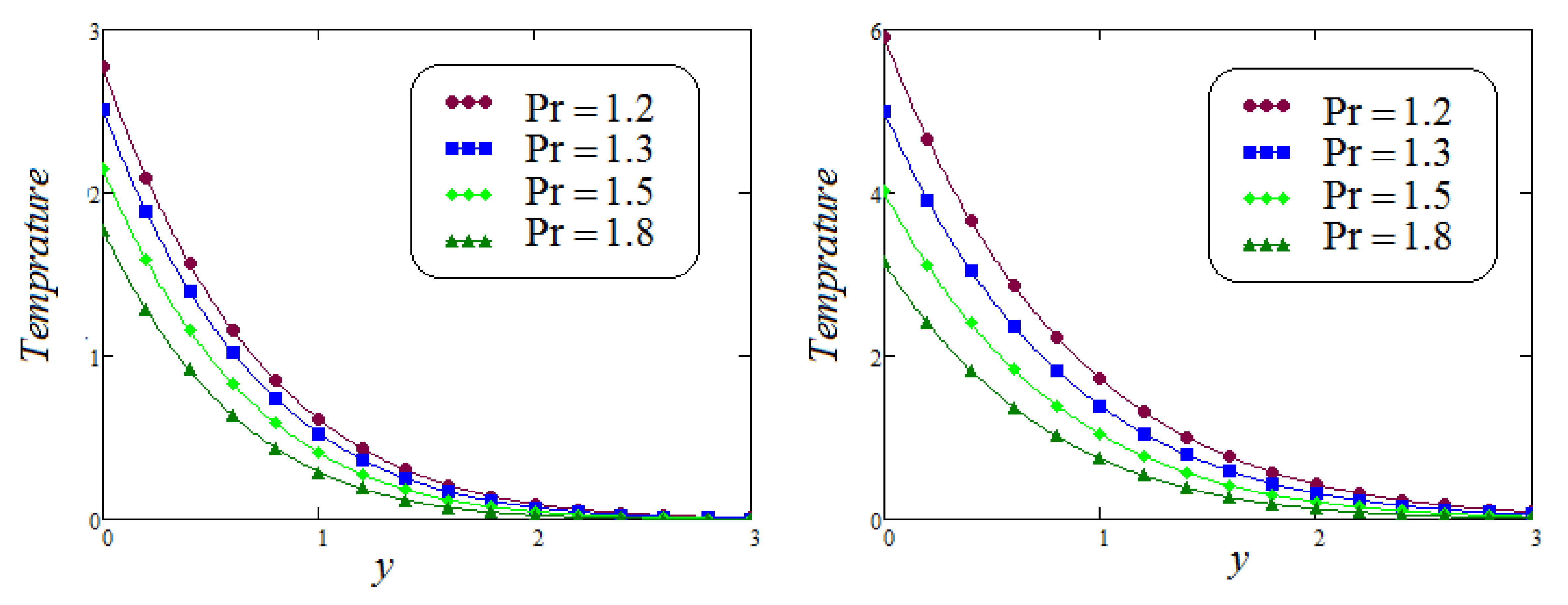
• The temperature graphs show that the temperature profile decreases for higher values of $Pr$.
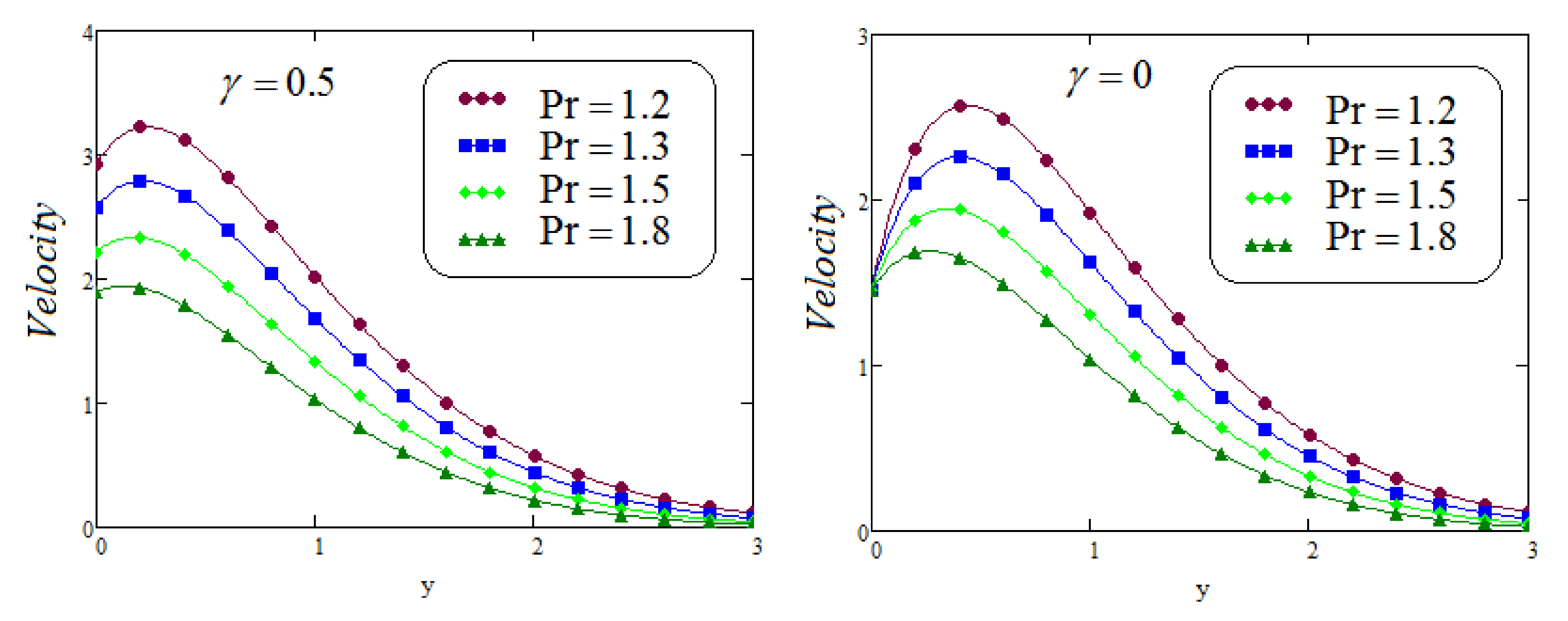
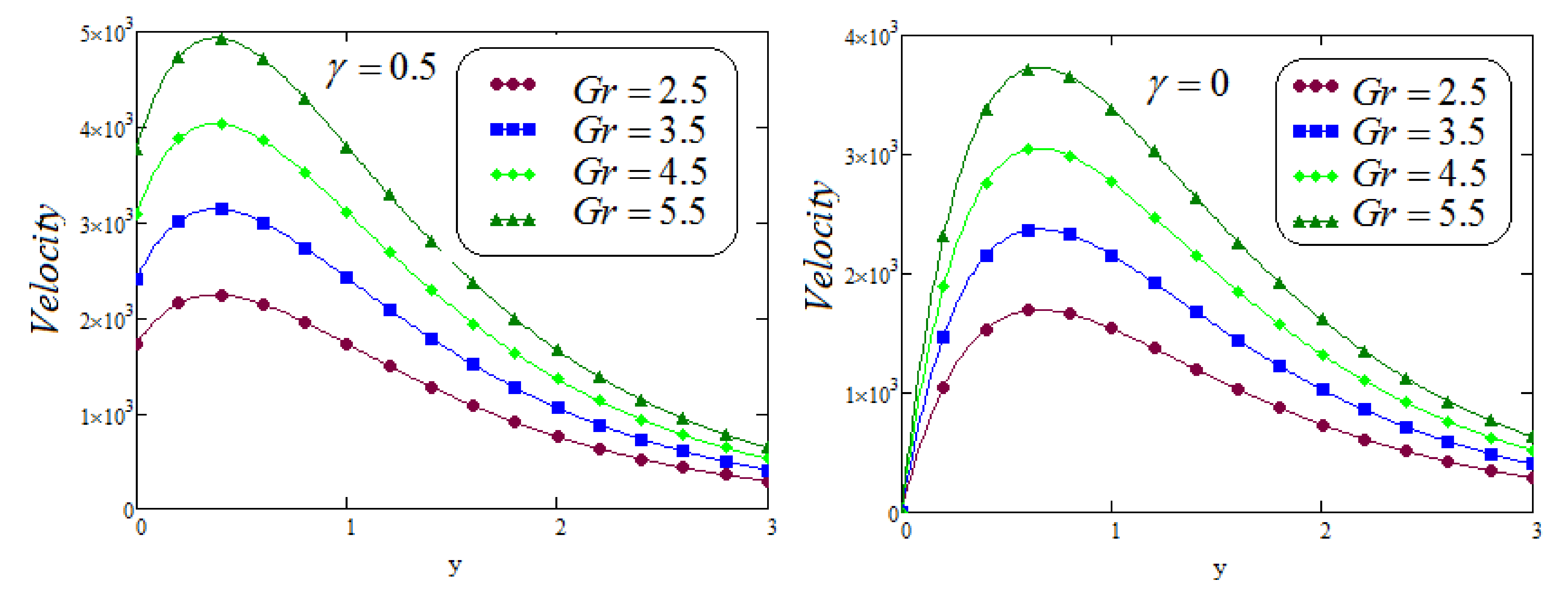
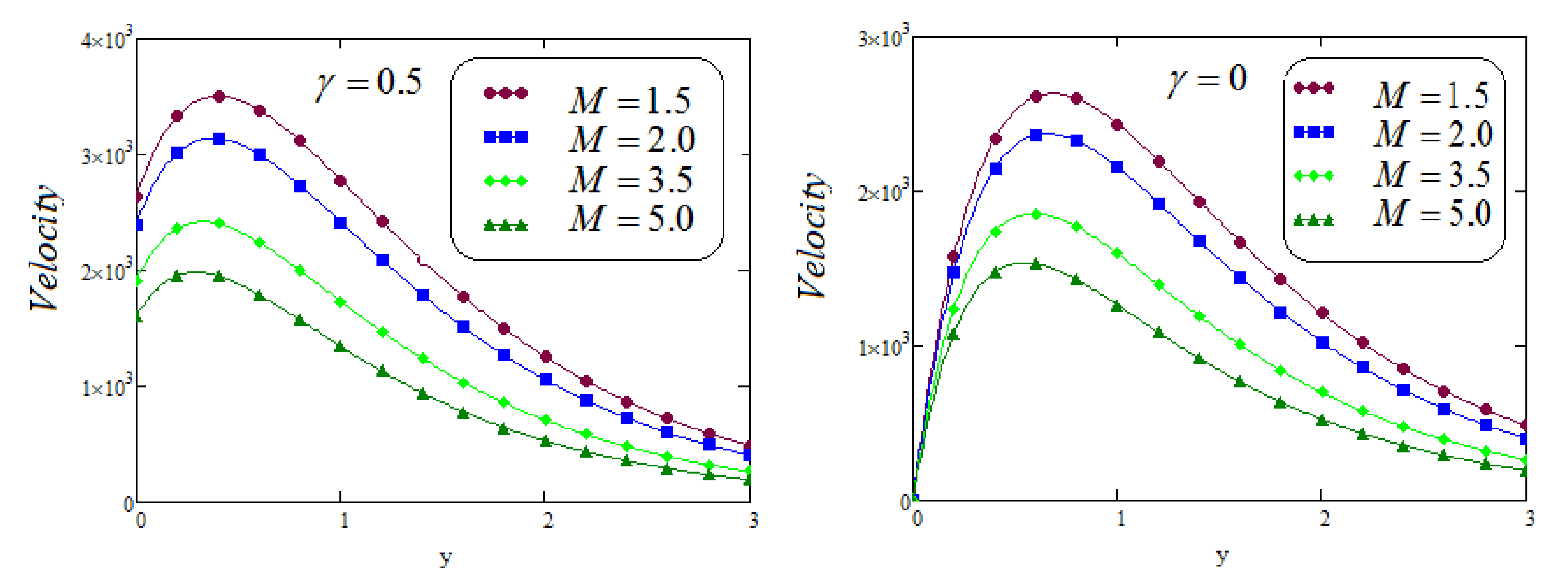
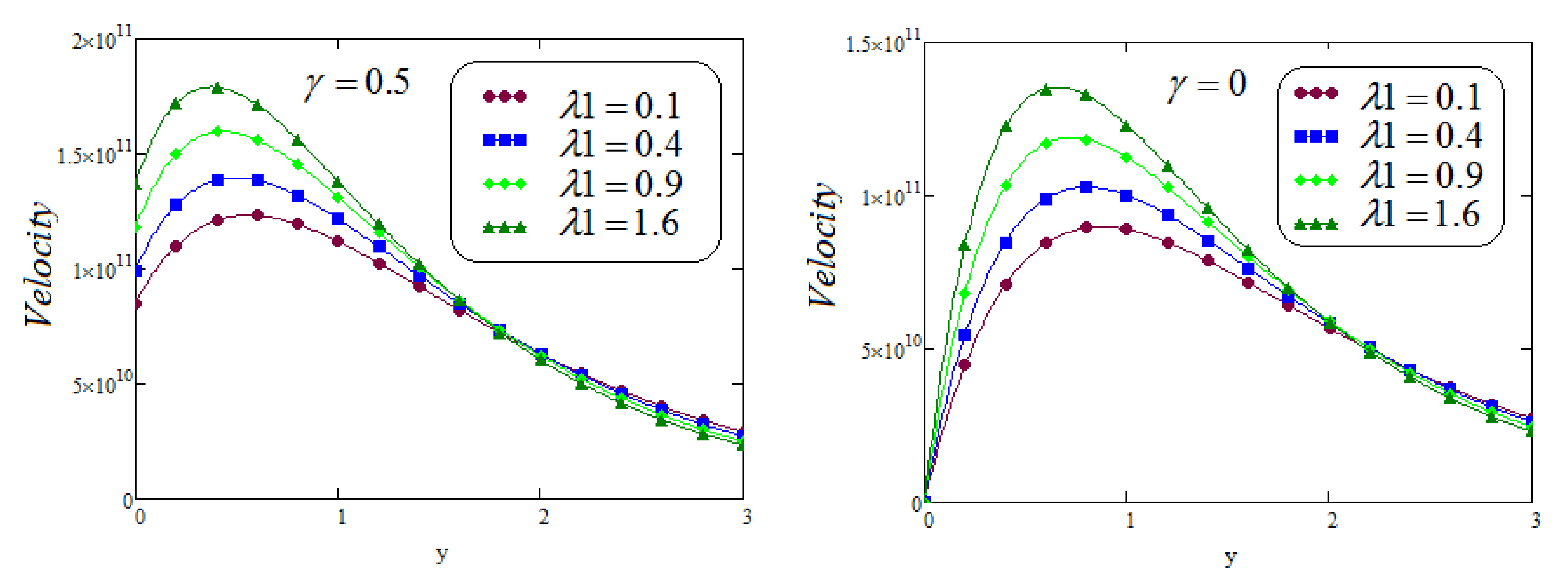
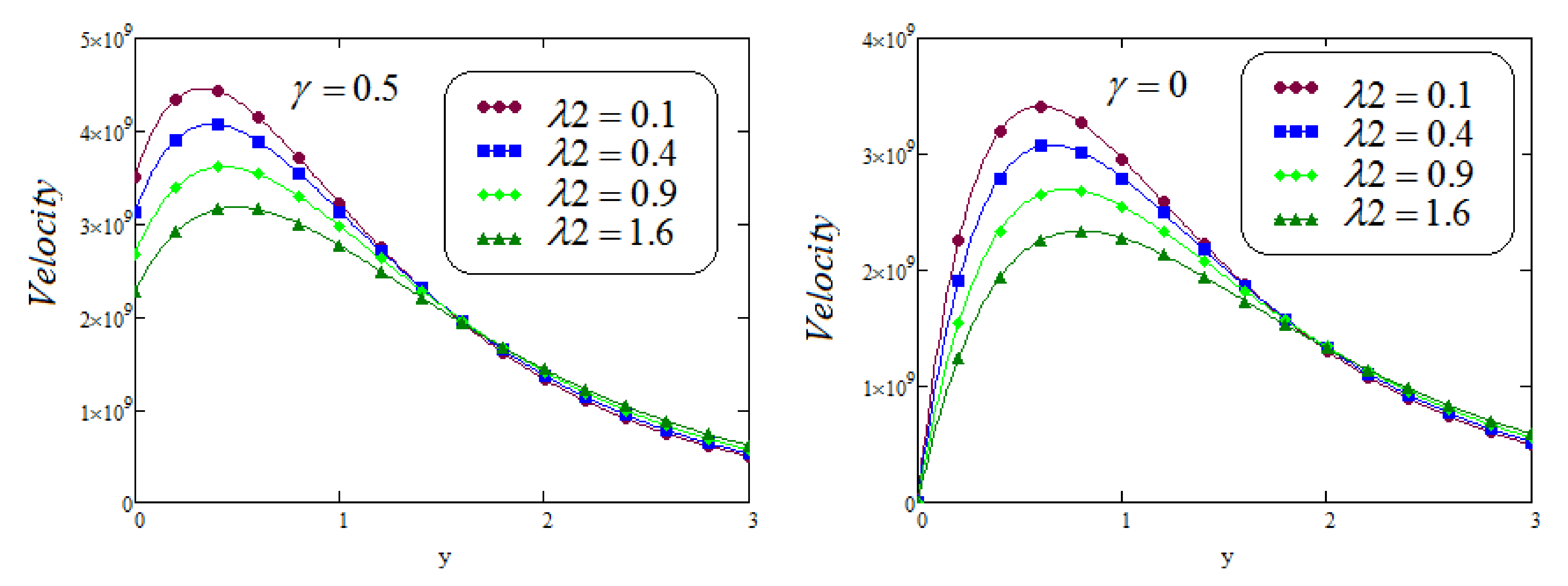
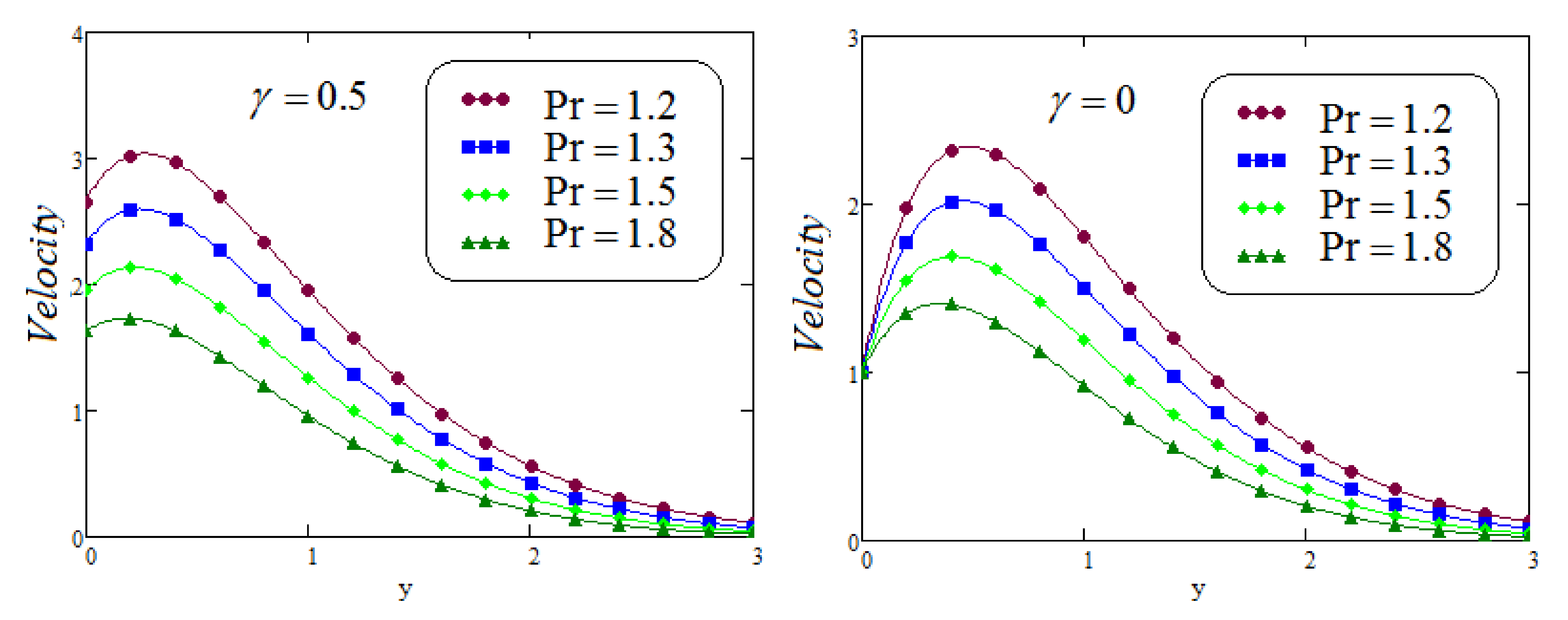
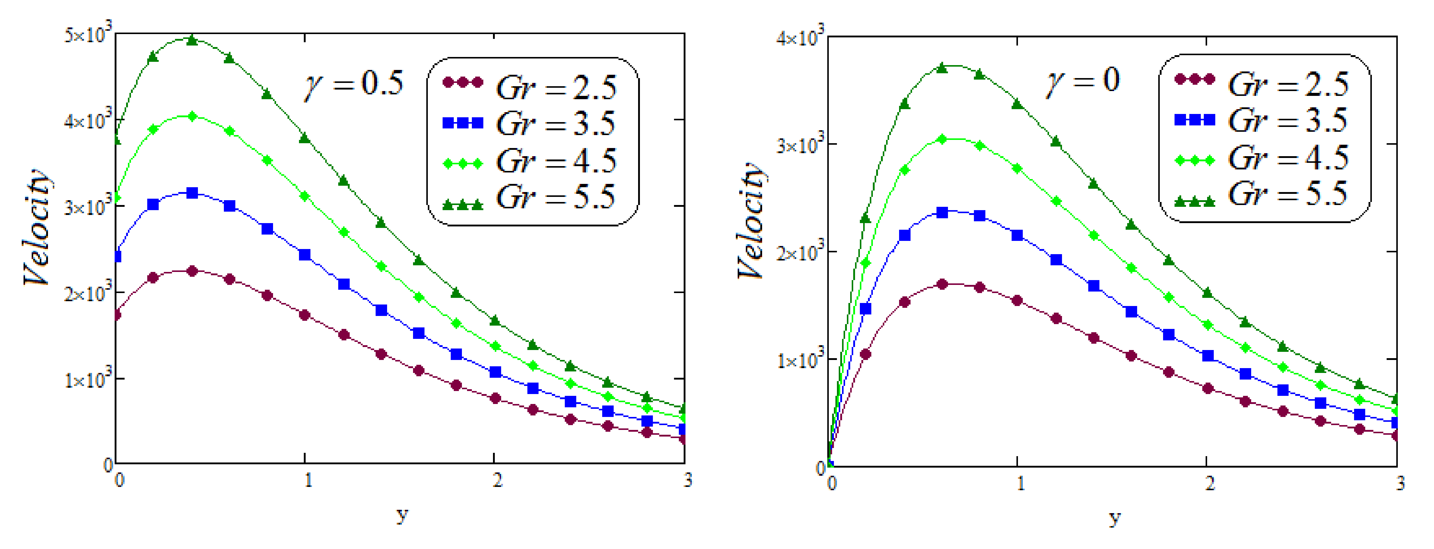
• The graphs for the velocity field under slip conditions as well as the velocity field under no-slip conditions show that the effects of ${\lambda }_1$ and ${\lambda }_2$ on the velocity contour are quite the opposite.
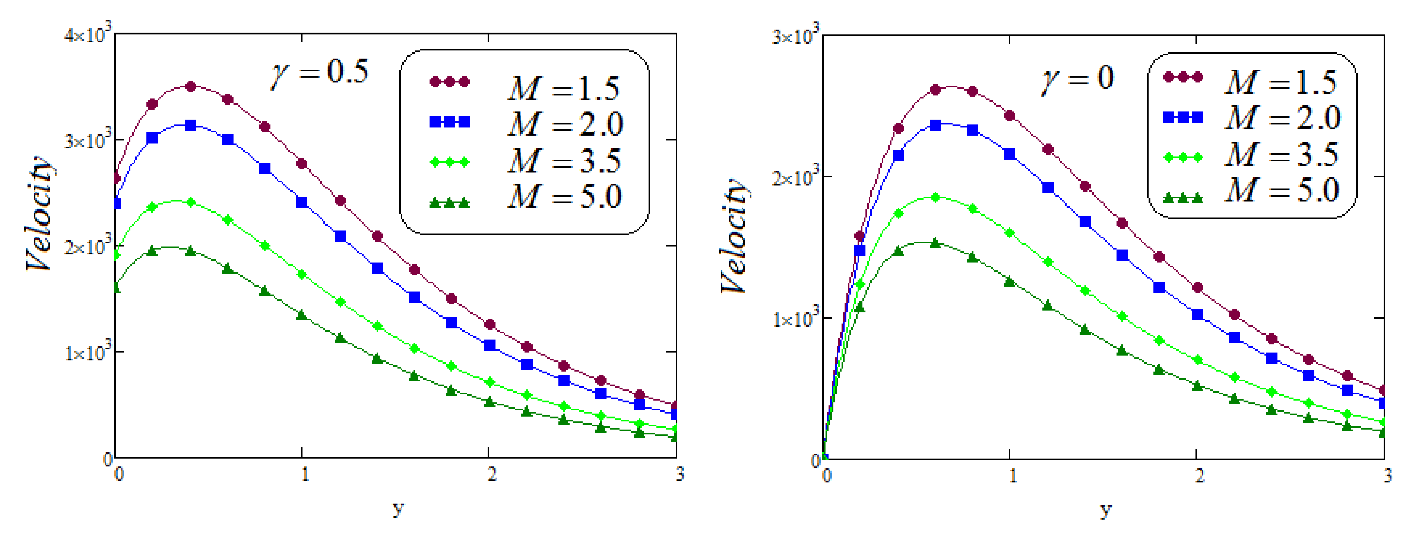
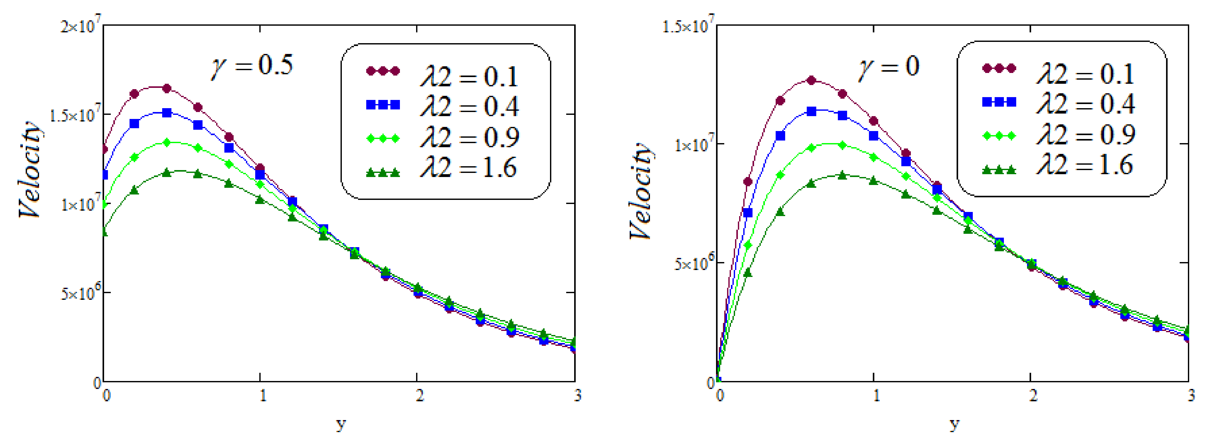
• From the graphs, one can see that the elevated values of M and $Pr$ reduced the velocity curve.
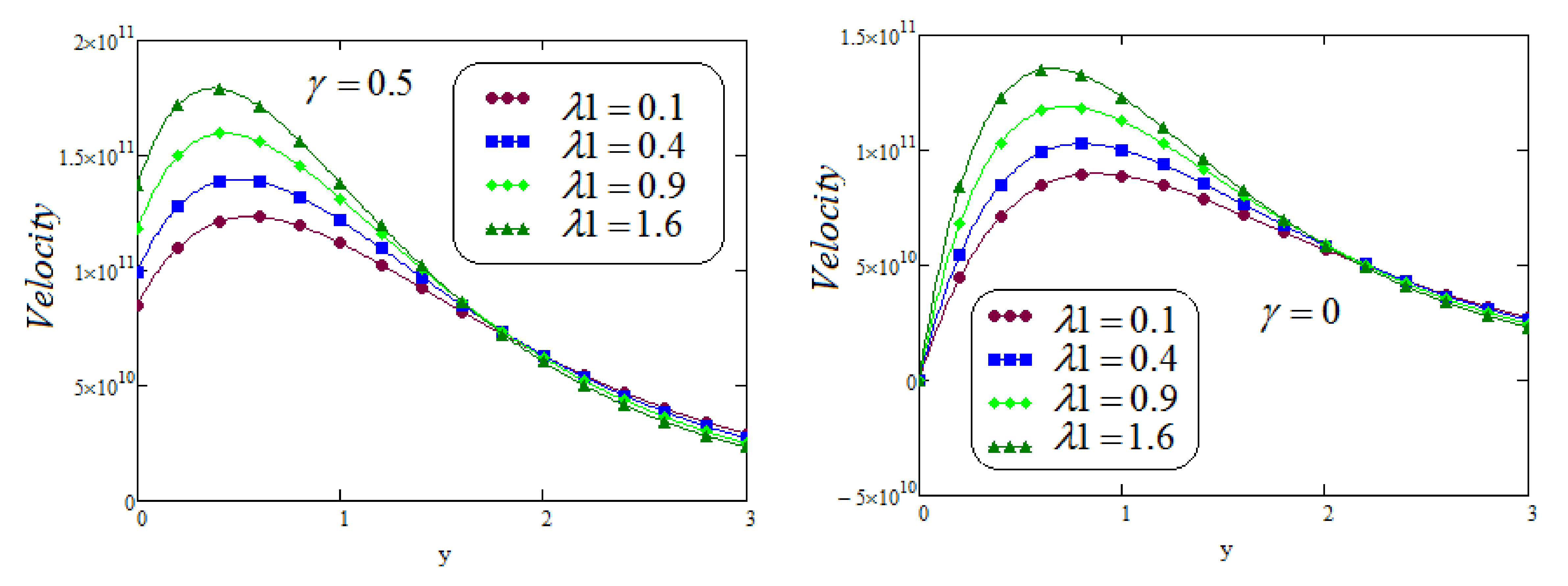
• The velocity profile was stimulated in function of the increasing values of $Gr$.
• It can be observed that the velocity profile for no-slip flow is lower than the velocity profile for slip flow.
• It was analyzed that for both functions $f\left(t\right)=e^{at}$ and $f\left(t\right)=sint$, the velocity field represents the same curve pattern for all the involved system parameters.

References

1. Kahshan, M.; Lu, D.; Siddiqui, A.M. A Jeffrey fluid model for a porous-walled channel: Application to flat plate dialyzer. Sci. Rep. 2019, 9, 15879. [Google Scholar] [CrossRef] [Green Version]
2. Farooq, U.; Lu, D.; Munir, S.; Ramzan, M.; Suleman, M.; Hussain, S. MHD flow of Maxwell fluid with nanomaterials due to an exponentially stretching surface. Sci. Rep. 2019, 9, 7312. [Google Scholar] [CrossRef] [Green Version]
3. Raza, N.; Awan, A.U.; Haque, E.; Abdullah, M.; Rashidi, M.M. Unsteady flow of a Burgers’ fluid with Caputo fractional derivatives: A hybrid technique. Ain Shams Eng. J. 2019, 10, 319–325. [Google Scholar] [CrossRef]
4. Shah, N.A.; Khan, I. Heat transfer analysis in a second grade fluid over and oscillating vertical plate using fractional Caputo-Fabrizio derivatives. Eur. Phys. J. C 2016, 76, 362. [Google Scholar] [CrossRef] [Green Version]
5. Khan, A.S.; Nie, Y.; Shah, Z. Impact of thermal radiation on magnetohydrodynamic unsteady thin film flow of Sisko fluid over a stretching surface. Processes 2019, 7, 369. [Google Scholar] [CrossRef] [Green Version]
6. Tanner, R.I. Note on the rayleigh problem for a visco–elastic fluid. Z. Angew. Math. Phys. 1962, 13, 573–580. [Google Scholar] [CrossRef]
7. Fetecau, C.; Prasad, S.C.; Rajagopal, K.R. A note on the flow induced by a constantly accelerating plate in an Oldroyd–B fluid. Appl. Math. Model. 2007, 31, 647–654. [Google Scholar] [CrossRef]
8. Fetecau, C.; Hayat, T.; Khan, M. Unsteady flow of an Oldroyd–B fluid induced by the impulsive motion of a plate between two side walls perpendicular to the plate. Acta Mech. 2008, 198, 21–33. [Google Scholar] [CrossRef]
9. Gul, T.; Islam, S.; Shah, R.A.; Khalid, A.; Khan, I.; Shafie, S. Unsteady MHD thin film flow of an Oldroyd–B fluid over an oscillating inclined belt. PLoS ONE 2015, 10, e0126698. [Google Scholar]
10. Tiwana, M.H.; Mann, A.B.; Rizwan, M.; Maqbool, K.; Javeed, S.; Raza, S.; Khan, M.S. Unsteady magnetohydrodynamic convective fluid flow of Oldroyd–B model considering ramped wall temperature and ramped wall velocity. Mathematics 2019, 7, 676. [Google Scholar] [CrossRef] [Green Version]
11. Wan, R. Some new global results to the incompressible Oldroyd–B model. Z. Angew. Math. Phys. 2019, 70, 28. [Google Scholar] [CrossRef]
12. Shakeel, A.; Ahmad, S.; Khan, H.; Shah, N.A.; Haq, S.U. Flows with slip of Oldroyd–B fluids over a moving plate. Adv. Math. Phys. 2016, 2016, 8619634. [Google Scholar] [CrossRef] [Green Version]
13. Tahir, M.; Naeem, M.N.; Javaid, M.; Younas, M.; Imran, M.; Sadiq, N.; Safdar, R. Unsteady flow of fractional Oldroyd–B fluids through rotating annulus. Open Phys. 2018, 16, 193–200. [Google Scholar] [CrossRef]
14. Wang, B.; Tahir, M.; Imran, M.; Javaid, M.; Jung, C.Y. Semi analytical solutions for fractional Oldroyd–B fluid through rotating annulus. IEEE Access 2019, 7, 72482–72491. [Google Scholar] [CrossRef]
15. Elhanafy, A.; Guaily, A.; Elsaid, A. Numerical simulation of Oldroyd–B fluid with application to hemodynamics. Adv. Mech. Eng. 2019, 11, 1–7. [Google Scholar] [CrossRef] [Green Version]
16. Ali, N.; Khan, S.U.; Sajid, M.; Abbas, Z. Flow and heat transfer of hydromagnetic Oldroyd–B fluid in a channel with stretching walls. Nonlinear Eng. 2016, 5, 73–79. [Google Scholar]
17. Chen, J.L.S.; Smith, T.N. Forced Convection Heat Transfer from Non-isothermal Thin Needles. J. Heat Transf. 1978, 100, 358–362. [Google Scholar] [CrossRef]
18. Jambal, O.; Shigechi, T.; Davaa, G.; Momoki, S. Effects of viscous dissipation and fluid axial heat conduction on heat transfer for non-Newtonian fluids in duct with uniform wall temperature. Int. Commun. Heat Mass Transf. 2005, 32, 1165–1173. [Google Scholar] [CrossRef]
19. Zan, W.; Lei, W.; Bengt, S. Pressure drop and convective heat transfer of water and nanofluids in a double-pipe helical heat exchanger. Appl. Therm. Eng. 2013, 60, 266–274. [Google Scholar]
20. Sheikholeslami, M.; Bandpy, M.G.; Ellahi, R.; Zeeshan, A. Simulation of MHD CuO-water nanofluid flow and convective heat transfer considering Lorentz forces. J. Magn. Magn. Mater. 2014, 369, 69–80. [Google Scholar] [CrossRef]
21. Kashif, A.A.; Mukarrum, H.; Mirza, M.B. An Analytic Study of Molybdenum Disulfide Nanofluids Using Modern Approach of Atangana-Baleanu Fractional Derivatives. Eur. Phys. J. Plus 2017, 132, 439. [Google Scholar] [CrossRef]
22. Bhojraj, L.; Abro, K.A.; Abdul, W.S. Thermodynamical analysis of heat transfer of gravity-driven fluid flow via fractional treatment: An analytical study. J. Therm. Anal. Calorim. 2020, 144, 155–165. [Google Scholar] [CrossRef]
23. Solangi, K.H.; Kazi, S.N.; Luhur, M.R.; Badarudin, A.; Amiri, A.; Sadri, R.; Zubir, M.N.M.; Gharehkhani, S.; Teng, K.H. A comprehensive review of thermo-physical properties and convective heat transfer to nanofluids. Energy 2015, 89, 1065e86. [Google Scholar] [CrossRef]
24. Shafiq, A.; Hammouch, Z.; Sindhu, T.N. Bioconvective MHD flow of tangent hyperbolic nanofluid with Newtonian heating. Int. J. Mech. Sci. 2017, 133, 759–766. [Google Scholar] [CrossRef]
25. Hamid, M.; Usman, M.; Khan, Z.H. Dual solutions and stability analysis of flow and heat transfer of Casson fluid over a stretching sheet. Phys. Lett. A 2019, 383, 2400–2408. [Google Scholar] [CrossRef]
26. Abdelmalek, Z.; Tayebi, T.; Dogonchi, A.S.; Chamkha, A.J.; Ganji, D.D.; Tlili, I. Role of various configurations of a wavy circular heater on convective heat transfer within an enclosure filled with nanofluid. Int. Commun. Heat Mass Transf. 2020, 113, 104525. [Google Scholar] [CrossRef]
27. Kashif, A.A. A Fractional and Analytic Investigation of Thermo-Diffusion Process on Free Convection Flow: An Application to Surface Modification Technology. Eur. Phys. J. Plus 2020, 135, 31. [Google Scholar] [CrossRef]
28. Reddy, M.G. Heat and mass transfer on magnetohydrodynamic peristaltic flow in a porous medium with partial slip. Alex. Eng. J. 2016, 55, 1225–1234. [Google Scholar] [CrossRef]
29. Abro, K.A.; Gomez-Aguilar, J.F. Fractional modeling of fin on non-Fourier heat conduction via modern fractional differential operators. Arab. J. Sci. Eng. 2021, 46, 2901–2910. [Google Scholar] [CrossRef]
30. Yin, C.; Zheng, L.; Zhang, C.; Zhang, X. Flow and heat transfer of nanofluids over a rotating disk with uniform stretching rate in the radial direction. Propuls. Power Res. 2017, 6, 25–30. [Google Scholar] [CrossRef]
31. Imran, M.A.; Riaz, M.B.; Shah, N.A.; Zafar, A.A. Boundary layer ow of MHD generalized Maxwell fluid over an exponentially accelerated infinite vertical surface with slip and Newtonian heating at the boundary. Results Phys. 2018, 8, 1061–1067. [Google Scholar] [CrossRef]
32. Kashif, A.A.; Abdon, A. Role of Non-integer and Integer Order Differentiations on the Relaxation Phenomena of Viscoelastic Fluid. Phys. Scr. 2020, 95, 035228. [Google Scholar] [CrossRef]
33. Shaheen, A.; Asjad, M.I. Peristaltic flow of a Sisko fluid over a convectively heated surface with viscous dissipation. J. Phys. Chem. Solids 2018, 122, 210–227. [Google Scholar] [CrossRef]
34. Rehman, A.U.; Riaz, M.B.; Saeed, S.T.; Yao, S. Dynamical Analysis of Radiation and Heat Transfer on MHD Second Grade Fluid. Comput. Model. Eng. Sci. 2021, 129, 689–703. [Google Scholar] [CrossRef]
35. Riaz, M.B.; Abro, K.A.; Abualnaja, K.M.; Akgül, A.; Rehman, A.U.; Abbas, M.; Hamed, Y.S. Exact solutions involving special functions for unsteady convective flow of magnetohydrodynamic second grade fluid with ramped conditions. Adv. Differ. Equ. 2021, 2021, 408. [Google Scholar] [CrossRef]
36. Abro, K.A. Numerical study and chaotic oscillations for aerodynamic model of wind turbine via fractal and fractional differential operators. Numer. Methods Partial. Differ. Equ. 2020, 2020, 1–15. [Google Scholar] [CrossRef]
37. Wakif, A.; Boulahia, Z.; Mishra, S.R.; Rashidi, M.M.; Sehaqui, R. Influence of a uniform transverse magnetic field on the thermohydrodynamic stability in water-based nanofluids with metallic nanoparticles using the generalized Buongiorno’s mathematical model. Eur. Phys. J. Plus 2018, 133, 181. [Google Scholar] [CrossRef]
38. Imran, M.A.; Aleem, M.; Riaz, M.B.; Ali, R.; Khan, I. A comprehensive report on convective flow of fractional (ABC) and (CF) MHD viscous fluid subject to generalized boundary conditions. Chaos Solitons Fractals 2018, 118, 274–289. [Google Scholar] [CrossRef]
39. Muhammad, A.; Makinde, O.D. Thermo-dynamic analysis of unsteady MHD mixed convection with slip and thermal radiation over a permeable surface. Defect Diffus. Forum 2017, 374, 29–46. [Google Scholar] [CrossRef]
40. Bhatti, M.M.; Rashidi, M.M. Study of heat and mass transfer with Joule heating on magnetohydrodynamic (MHD) peristaltic blood flow under the influence of Hall effect. Propuls Power Res. 2017, 6, 177–185. [Google Scholar] [CrossRef]
41. Memon, I.Q.; Abro, K.A.; Solangi, M.A.; Shaikh, A.A. Functional shape effects of nanoparticles on nanofluid suspended in ethylene glycol through Mittage-Leffler approach. Phys. Scr. 2020, 96, 025005. [Google Scholar] [CrossRef]
42. Abro, K.A. Fractional characterization of fluid and synergistic effects of free convective flow in circular pipe through Hankel transform. Phys. Fluids 2020, 32, 123102. [Google Scholar] [CrossRef]
43. Riaz, M.B.; Awrejcewicz, J.; Rehman, A.U.; Akgül, A. Thermophysical Investigation of Oldroyd-B Fluid with Functional Effects of Permeability: Memory Effect Study Using Non-Singular Kernel Derivative Approach. Fractal Fract. 2021, 5, 124. [Google Scholar] [CrossRef]
44. Riaz, M.B.; Saeed, S.T.; Baleanu, D.; Ghalib, M. Computational results with non-singular and non-local kernel flow of viscous fluid in vertical permeable medium with variant temperature. Front. Phys. 2020, 8, 275. [Google Scholar] [CrossRef]
45. Abro, K.A.; Atangana, A. Dual fractional modeling of rate type fluid through non-local differentiation. Numer. Methods Partial. Differ. Equ. 2020, 2020, 1–16. [Google Scholar] [CrossRef]
46. Afridi, M.I.; Qasim, M.; Wakif, A.; Hussanan, A. Second law analysis of dissipative nanofluid flow over a curved surface in the presence of Lorentz force: Utilization of the Chebyshev–Gauss–Lobatto spectral method. Nanomaterials 2019, 9, 195. [Google Scholar] [CrossRef] [Green Version]
47. Abro, K.A.; Atangana, A. Numerical and mathematical analysis of induction motor by means of AB–fractal–fractional differentiation actuated by drilling system. Numer. Methods Partial. Differ. Equ. 2020, 1–15. [Google Scholar] [CrossRef]
48. Abro, K.A.; Siyal, A.; Souayeh, B.; Atangana, A. Application of Statistical Method on Thermal Resistance and Conductance during Magnetization of Fractionalized Free Convection Flow. Int. Commun. Heat Mass Transf. 2020, 119, 104971. [Google Scholar] [CrossRef]
49. Abro, K.A.; Soomro, M.; Atangana, A.; Gómez-Aguilar, J.F. Thermophysical properties of Maxwell Nanoluids via fractional derivatives with regular kernel. J. Therm. Anal. Calorim. 2020. [Google Scholar] [CrossRef]
50. Rehman, A.U.; Riaz, M.B.; Awrejcewicz, J.; Baleanu, D. Exact solutions of thermomagetized unsteady non-singularized jeffery fluid: Effects of ramped velocity, concentration with newtonian heating. Results Phys. 2021, 26, 104367. [Google Scholar] [CrossRef]
51. Rehman, A.U.; Riaz, M.B.; Akgul, A.; Saeed, S.T.; Baleanu, D. Heat and mass transport impact on MHD second grade fluid: A comparative analysis of fractional operators. Heat Transf. 2021, 50, 7042–7064. [Google Scholar] [CrossRef]
52. Zhu, Y.; Granick, S. Limits of the hydrodynamic no-slip boundary condition. Phys. Rev. Lett. 2002, 88, 106102. [Google Scholar] [CrossRef] [Green Version]
53. Navier, C.L.M.H. Memoire surles du movement des. Mem. Acad. Sci. Inst. Fr. 1823, 1, 414–416. [Google Scholar]
54. Blake, T.D. Slip between a liquid and a solid: DM Tolstoi’s (1952) theory reconsidered. Colloids Surf. 1990, 47, 135–145. [Google Scholar] [CrossRef]
55. Pit, R.; Hervet, H.; Leger, L. Friction and slip of a simple liquid at a solid surface. Tribol. Lett. 1999, 7, 147–152. [Google Scholar] [CrossRef]
56. Asghar, S.; Parveen, S.; Hanif, S.; Siddiqui, A.M.; Hayat, T. Hall effects on the unsteady hydromagnetic flows of an Oldroyd–B fluid. Int. J. Eng. Sci. 2003, 41, 609–619. [Google Scholar] [CrossRef]
57. Anwar, T.; Khan, I.; Kumam, P.; Watthayu, W. Impacts of thermal radiation and heat consumption/generation on unsteady MHD convection flow of an Oldroyd–B fluid with ramped velocity and temperature in a generalized Darcy medium. Mathematics 2020, 8, 130. [Google Scholar] [CrossRef] [Green Version]
58. Martyushev, S.G.; Sheremet, M.A. Characteristics of Rosseland and P-1 approximations in modeling nonstationary conditions of convection-radiation heat transfer in an enclosure with a local energy source. J. Eng. Thermophys. 2012, 21, 111–118. [Google Scholar] [CrossRef]
59. Ghalib, M.M.; Zafar, A.A.; Farman1, M.; Akgul, A.; Ahmad, M.O.; Ahmad, A. Unsteady MHD flow of Maxwell fluid with (CF) non-integer derivative model having slip/non-slip fluid flow and Newtonian heating at the boundary. Indian J. Phys. 2021. [Google Scholar] [CrossRef]
Figure 1. Geometry of the considered model.
Applsci 11 11477 g001
Figure 2. Temperature profile using different P r values, when t = 0.9 and t = 1.5 .
Applsci 11 11477 g002
Figure 3. Velocity field under slip conditions as well as the velocity field under no-slip conditions for different P r values when f ( t ) = e a t , a = 0.25 , t = 1.5 , G r = 3.5 , λ 1 = 0.6 , λ 2 = 0.2 , M = 2 .
Applsci 11 11477 g003
Figure 4. Velocity field under slip conditions as well as the velocity field under no-slip conditions for different G r values when f ( t ) = e a t , a = 0.25 , t = 1.5 , P r = 0.71 , λ 1 = 0.6 , λ 2 = 0.2 , M = 2 .
Applsci 11 11477 g004
Figure 5. Velocity field under slip conditions as well as the velocity field under no-slip conditions for different M values when f ( t ) = e a t , a = 0.25 , t = 1.5 , G r = 3.5 , λ 1 = 0.6 , λ 2 = 0.2 , P r = 0.71 .
Applsci 11 11477 g005
Figure 6. Velocity field under slip conditions as well as the velocity field under no-slip conditions for different λ 1 values when f ( t ) = e a t , a = 0.25 , t = 1.5 , G r = 3.5 , P r = 0.71 , λ 2 = 0.2 , M = 2 .
Applsci 11 11477 g006
Figure 7. Velocity field under slip conditions as well as the velocity field under no-slip conditions for different λ 2 values when f ( t ) = e a t , a = 0.25 , t = 1.5 , G r = 3.5 , λ 1 = 0.6 , P r = 0.71 , M = 2 .
Applsci 11 11477 g007
Figure 8. Velocity field under slip conditions as well as the velocity field under no-slip conditions for different P r values when f ( t ) = s i n t , t = 1.5 , G r = 3.5 , λ 1 = 0.6 , λ 2 = 0.2 , M = 2 .
Applsci 11 11477 g008
Figure 9. Velocity field under slip conditions as well as the velocity field under no-slip conditions for different G r values when f ( t ) = s i n t , t = 1.5 , P r = 0.71 , λ 1 = 0.6 , λ 2 = 0.2 , M = 2 .
Applsci 11 11477 g009
Figure 10. Velocity field under slip conditions as well as the velocity field under no-slip conditions for different M values when f ( t ) = s i n t , t = 1.5 , G r = 3.5 , λ 1 = 0.6 , λ 2 = 0.2 , P r = 0.71 .
Applsci 11 11477 g010
Figure 11. Velocity field under slip conditions as well as the velocity field under no-slip conditions for different λ 1 values when f ( t ) = s i n t , t = 1.5 , G r = 3.5 , P r = 0.71 , λ 2 = 0.2 , M = 2 .
Applsci 11 11477 g011
Figure 12. Velocity field under slip conditions as well as the velocity field under no-slip conditions for different λ 2 values when f ( t ) = s i n t , t = 1.5 , G r = 3.5 , λ 1 = 0.6 , P r = 0.71 , M = 2 .
Applsci 11 11477 g012
Publisher’s Note: MDPI stays neutral with regard to jurisdictional claims in published maps and institutional affiliations.