
Quantum-Inspired Classification Algorithm from DBSCAN–Deutsch–Jozsa Support Vectors and Ising Prediction Model

 ,
,
Abstract
:1. Introduction
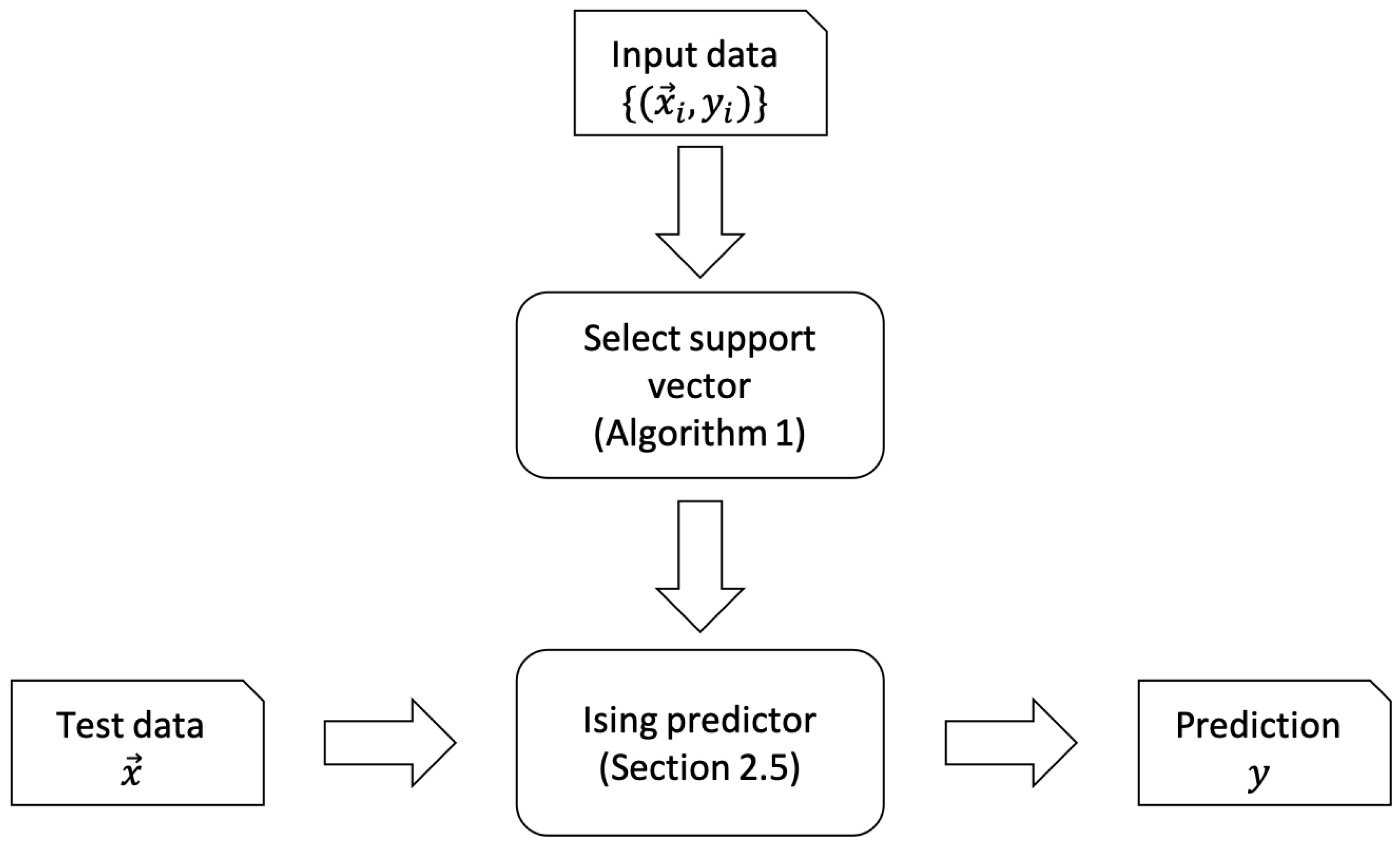
2. The Learning Algorithm
2.1. Hypothesis Set
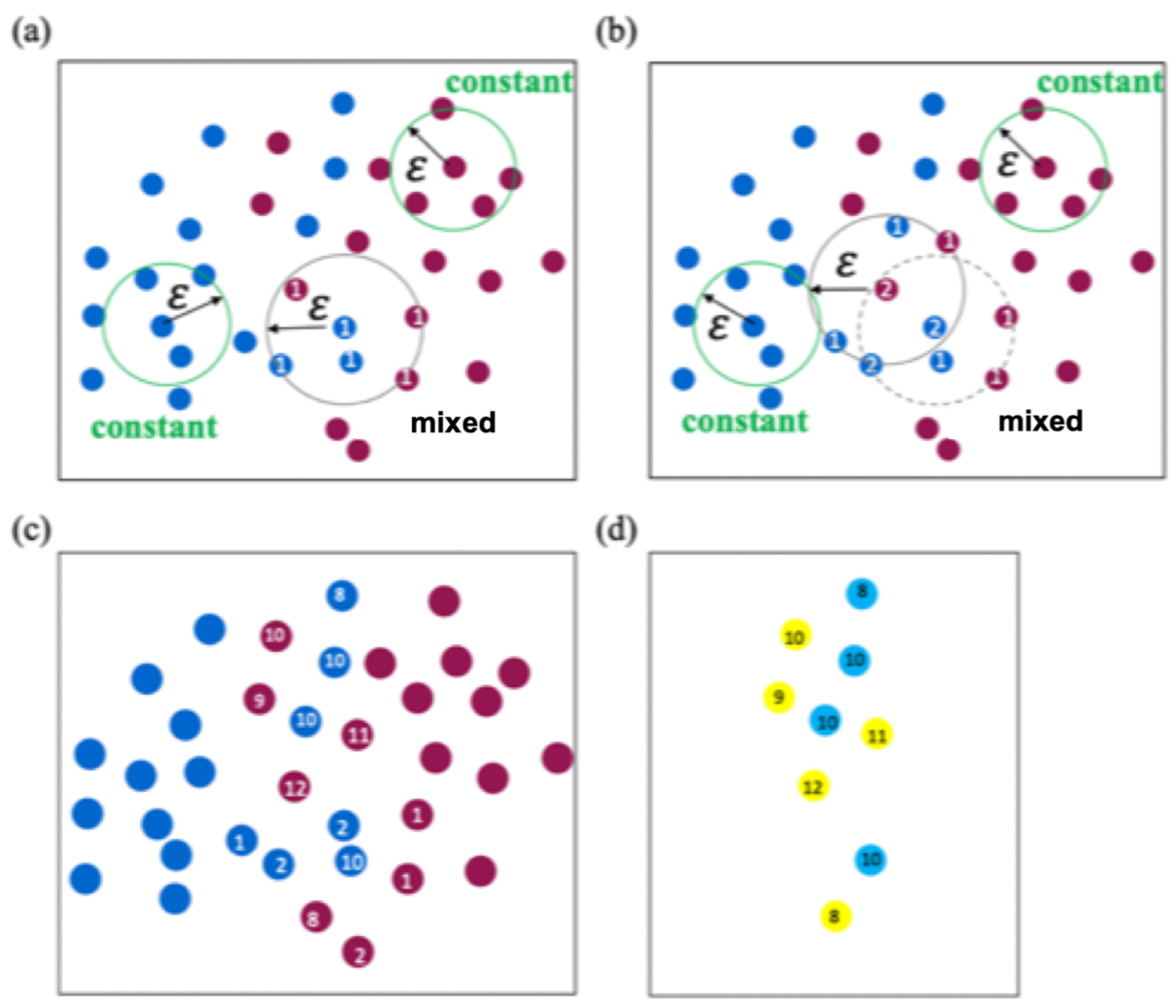
2.2. DBSCAN Algorithm for Determining the Support Vector
| Algorithm 1: The training algorithm to determine support vectors. |
 |
2.3. Integer Linear Programming Formulation
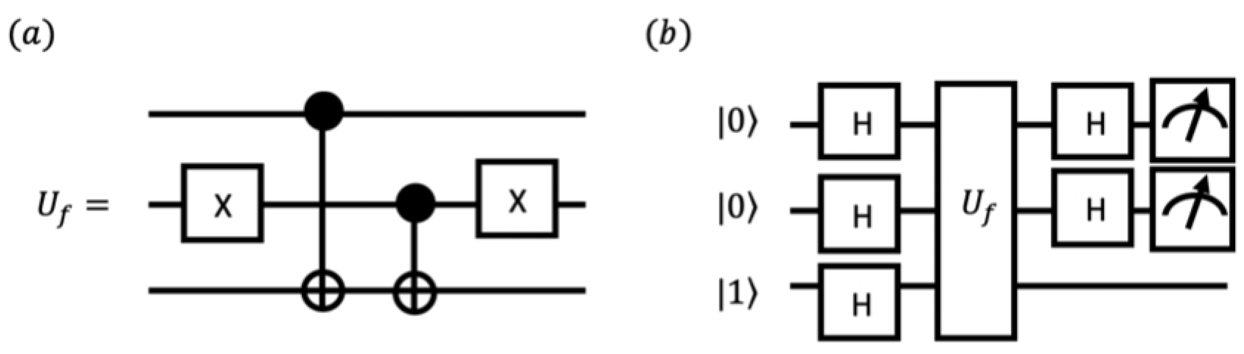
2.4. Quantum-Enhanced Algorithm with DJ
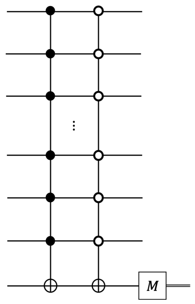
2.5. Annealing Algorithm for Data Prediction
2.6. The VC Dimension
3. Simulation Results
4. Computational Complexity
5. Conclusions
Author Contributions
Funding
Institutional Review Board Statement
Informed Consent Statement
Data Availability Statement
Acknowledgments
Conflicts of Interest
Appendix A. VC Dimension of Ising Predictor
References
- Schuld, M.; Sinayskiy, I.; Petruccione, F. An introduction to quantum machine learning. Contemp. Phys. 2015, 56, 172–185. [Google Scholar] [CrossRef] [Green Version]
- Biamonte, J.; Wittek, P.; Pancotti, N.; Rebentrost, P.; Wiebe, N.; Lloyd, S. Quantum machine learning. Nature 2017, 549, 195–202. [Google Scholar] [CrossRef] [PubMed]
- Aaronson, S. The learnability of quantum states. Proc. R. Soc. A Math. Phys. Eng. Sci. 2007, 463, 3089–3114. [Google Scholar] [CrossRef] [Green Version]
- Dumoulin, V.; Goodfellow, I.J.; Courville, A.; Bengio, Y. On the Challenges of Physical Implementations of RBMs. In Proceedings of the Twenty-Eighth AAAI Conference on Artificial Intelligence (AAAI’14), Quebec City, QC, Canada, 27–31 July 2014; pp. 1199–1205. [Google Scholar]
- Romero, J.; Olson, J.P.; Aspuru-Guzik, A. Quantum autoencoders for efficient compression of quantum data. Quantum Sci. Technol. 2017, 2, 045001. [Google Scholar] [CrossRef] [Green Version]
- Crawford, D.; Levit, A.; Ghadermarzy, N.; Oberoi, J.S.; Ronagh, P. Reinforcement Learning Using Quantum Boltzmann Machines. Quantum Inf. Comput. 2018, 18, 51–74. [Google Scholar] [CrossRef]
- Mitarai, K.; Negoro, M.; Kitagawa, M.; Fujii, K. Quantum circuit learning. Phys. Rev. A 2018, 98, 032309. [Google Scholar] [CrossRef] [Green Version]
- Chen, C.C.; Watabe, M.; Shiba, K.; Sogabe, M.; Sakamoto, K.; Sogabe, T. On the expressibility and overfitting of quantum circuit learning. ACM Trans. Quantum Comput. 2021, 2, 1–24. [Google Scholar] [CrossRef]
- Harrow, A.W.; Hassidim, A.; Lloyd, S. Quantum Algorithm for Linear Systems of Equations. Phys. Rev. Lett. 2009, 103, 150502. [Google Scholar] [CrossRef]
- Borle, A.; Elfving, V.E.; Lomonaco, S.J. Quantum Approximate Optimization for Hard Problems in Linear Algebra. arXiv 2020, arXiv:2006.15438. [Google Scholar] [CrossRef]
- Lin, L.; Tong, Y. Optimal polynomial based quantum eigenstate filtering with application to solving quantum linear systems. Quantum 2020, 4, 361. [Google Scholar] [CrossRef]
- Harrow, A.W. Small quantum computers and large classical data sets. arXiv 2020, arXiv:2004.00026. [Google Scholar]
- Aaronson, S. Read the fine print. Nat. Phys. 2015, 11, 291–293. [Google Scholar] [CrossRef]
- Nakaji, K.; Yamamoto, N. Quantum semi-supervised generative adversarial network for enhanced data classification. arXiv 2020, arXiv:2010.13727. [Google Scholar] [CrossRef]
- Preskill, J. Quantum Computing in the NISQ era and beyond. Quantum 2018, 2, 79. [Google Scholar] [CrossRef]
- Tang, E. A Quantum-Inspired Classical Algorithm for Recommendation Systems. In Proceedings of the 51st Annual ACM SIGACT Symposium on Theory of Computing (STOC 2019), Phoenix, AZ, USA, 23–26 June 2019; Association for Computing Machinery: New York, NY, USA, 2019; pp. 217–228. [Google Scholar] [CrossRef] [Green Version]
- Chia, N.H.; Li, T.; Lin, H.H.; Wang, C. Quantum-inspired sublinear algorithm for solving low-rank semidefinite programming. arXiv 2019, arXiv:1901.03254. [Google Scholar]
- Arrazola, J.M.; Delgado, A.; Bardhan, B.R.; Lloyd, S. Quantum-inspired algorithms in practice. Quantum 2020, 4, 307. [Google Scholar] [CrossRef]
- Bravyi, S.; Kliesch, A.; Koenig, R.; Tang, E. Hybrid quantum-classical algorithms for approximate graph coloring. arXiv 2020, arXiv:2011.13420. [Google Scholar]
- Chia, N.H.; Gilyén, A.; Li, T.; Lin, H.H.; Tang, E.; Wang, C. Sampling-Based Sublinear Low-Rank Matrix Arithmetic Framework for Dequantizing Quantum Machine Learning. In Proceedings of the 52nd Annual ACM SIGACT Symposium on Theory of Computing (STOC 2020), Chicago, IL, USA, 22–26 July 2020; Association for Computing Machinery: New York, NY, USA, 2020; pp. 387–400. [Google Scholar] [CrossRef]
- Cortes, C.; Vapnik, V. Support-Vector Networks. Mach. Learn. 1995, 20, 273–297. [Google Scholar] [CrossRef]
- Chang, C.C.; Lin, C.J. LIBSVM: A Library for Support Vector Machines. ACM Trans. Intell. Syst. Technol. 2011, 2, 1–27. [Google Scholar] [CrossRef]
- Pedregosa, F.; Varoquaux, G.; Gramfort, A.; Michel, V.; Thirion, B.; Grisel, O.; Blondel, M.; Prettenhofer, P.; Weiss, R.; Dubourg, V.; et al. Scikit-learn: Machine Learning in Python. J. Mach. Learn. Res. 2011, 12, 2825–2830. [Google Scholar]
- Bordes, A.; Ertekin, S.; Weston, J.; Bottou, L. Fast Kernel Classifiers with Online and Active Learning. J. Mach. Learn. Res. 2005, 6, 1579–1619. [Google Scholar]
- Wu, X.; Zuo, W.; Lin, L.; Jia, W.; Zhang, D. F-SVM: Combination of Feature Transformation and SVM Learning via Convex Relaxation. IEEE Trans. Neural Netw. Learn. Syst. 2018, 29, 5185–5199. [Google Scholar] [CrossRef] [Green Version]
- Rizwan, A.; Iqbal, N.; Ahmad, R.; Kim, D.H. WR-SVM Model Based on the Margin Radius Approach for Solving the Minimum Enclosing Ball Problem in Support Vector Machine Classification. Appl. Sci. 2021, 11, 4657. [Google Scholar] [CrossRef]
- Rebentrost, P.; Mohseni, M.; Lloyd, S. Quantum Support Vector Machine for Big Data Classification. Phys. Rev. Lett. 2014, 113, 130503. [Google Scholar] [CrossRef]
- Schuld, M.; Fingerhuth, M.; Petruccione, F. Implementing a distance-based classifier with a quantum interference circuit. EPL (Europhys. Lett.) 2017, 119, 60002. [Google Scholar] [CrossRef] [Green Version]
- Havlíček, V.; Córcoles, A.D.; Temme, K.; Harrow, A.W.; Kandala, A.; Chow, J.M.; Gambetta, J.M. Supervised learning with quantum-enhanced feature spaces. Nature 2019, 567, 209–212. [Google Scholar] [CrossRef] [Green Version]
- Ester, M.; Kriegel, H.P.; Sander, J.; Xu, X. A Density-Based Algorithm for Discovering Clusters in Large Spatial Databases with Noise. In Proceedings of the Second International Conference on Knowledge Discovery and Data Mining (KDD’96), Portland, OR, USA, 2–4 August 1996; pp. 226–231. [Google Scholar]
- Deutsch, D.; Jozsa, R. Rapid solution of problems by quantum computation. Proc. R. Soc. Lond. Ser. A Math. Phys. Sci. 1992, 439, 553–558. [Google Scholar] [CrossRef]
- Rasmussen, S.E.; Groenland, K.; Gerritsma, R.; Schoutens, K.; Zinner, N.T. Single-step implementation of high-fidelity n-bit Toffoli gates. Phys. Rev. A 2020, 101, 022308. [Google Scholar] [CrossRef] [Green Version]
- Farhi, E.; Goldstone, J.; Gutmann, S.; Sipser, M. Quantum Computation by Adiabatic Evolution. arXiv 2000, arXiv:quant-ph/quant-ph/0001106. [Google Scholar]
- Kadowaki, T.; Nishimori, H. Quantum annealing in the transverse Ising model. Phys. Rev. E 1998, 58, 5355–5363. [Google Scholar] [CrossRef] [Green Version]
- Bishop, C.M. Pattern Recognition and Machine Learning (Information Science and Statistics); Springer: Berlin/Heidelberg, Germany, 2006. [Google Scholar]
- Giri, K.; Biswas, T.K.; Sarkar, P. ECR-DBSCAN: An improved DBSCAN based on computational geometry. Mach. Learn. Appl. 2021, 6, 100148. [Google Scholar] [CrossRef]


| 00 | −1 | 0 |
| 01 | 1 | 1 |
| 10 | 1 | 1 |
| 11 | −1 | 0 |
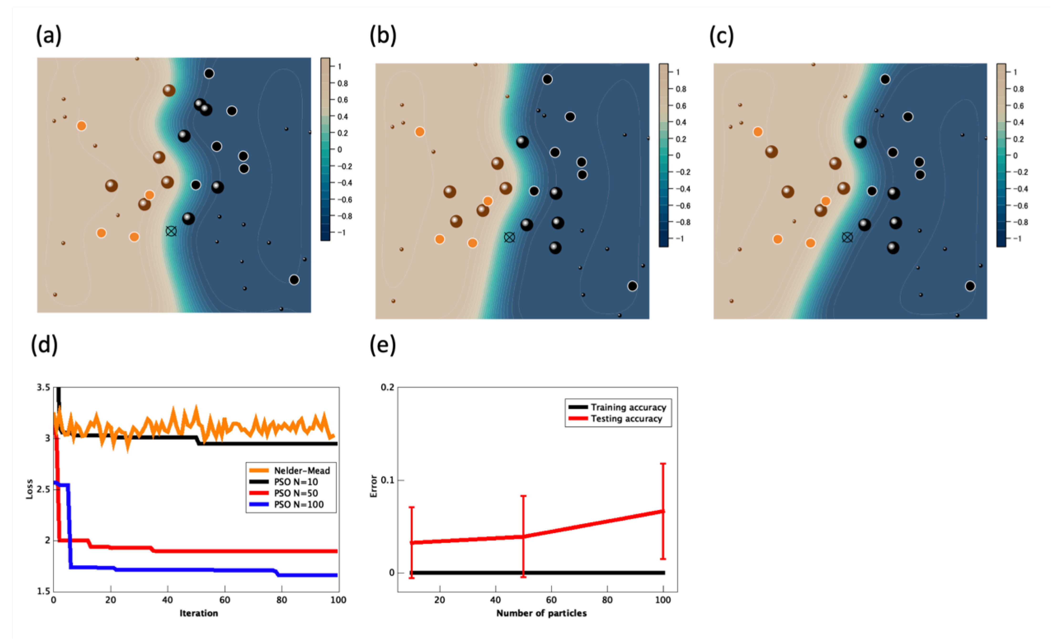
| N | Test Accuracy | |
|---|---|---|
| 10 | 1.128 | 0.9675 |
| 50 | 0.6356 | 0.9610 |
| 100 | 0.6157 | 0.9335 |
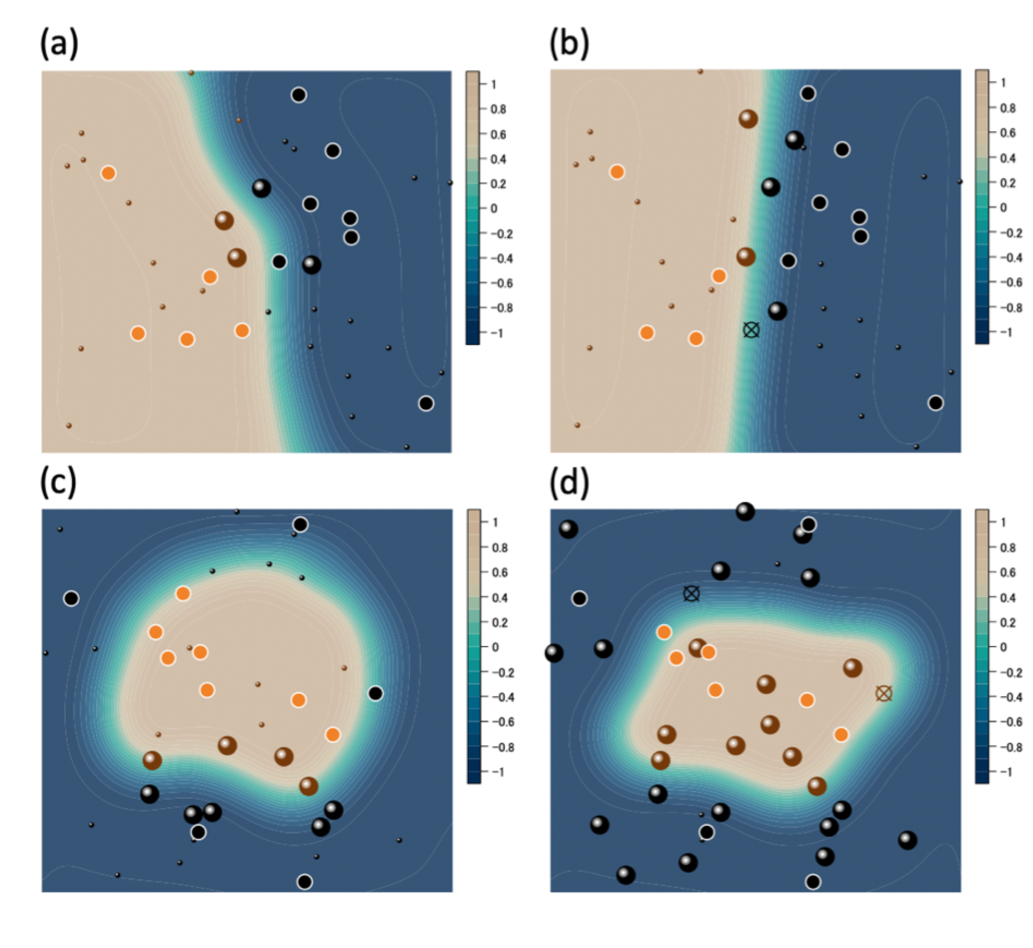
| Data | Total | +1 Label | Label |
|---|---|---|---|
| Linear Training | 28 | 13 | 15 |
| Linear Testing | 12 | 5 | 7 |
| Non-linear Training | 28 | 9 | 19 |
| Non-linear Testing | 12 | 7 | 5 |
| Training | Prediction | |
|---|---|---|
| Kernel SVM | ||
| This work |
Publisher’s Note: MDPI stays neutral with regard to jurisdictional claims in published maps and institutional affiliations. |
© 2021 by the authors. Licensee MDPI, Basel, Switzerland. This article is an open access article distributed under the terms and conditions of the Creative Commons Attribution (CC BY) license (https://creativecommons.org/licenses/by/4.0/).
Share and Cite
Shiba, K.; Chen, C.-C.; Sogabe, M.; Sakamoto, K.; Sogabe, T. Quantum-Inspired Classification Algorithm from DBSCAN–Deutsch–Jozsa Support Vectors and Ising Prediction Model. Appl. Sci. 2021, 11, 11386. https://doi.org/10.3390/app112311386
Shiba K, Chen C-C, Sogabe M, Sakamoto K, Sogabe T. Quantum-Inspired Classification Algorithm from DBSCAN–Deutsch–Jozsa Support Vectors and Ising Prediction Model. Applied Sciences. 2021; 11(23):11386. https://doi.org/10.3390/app112311386
Chicago/Turabian StyleShiba, Kodai, Chih-Chieh Chen, Masaru Sogabe, Katsuyoshi Sakamoto, and Tomah Sogabe. 2021. "Quantum-Inspired Classification Algorithm from DBSCAN–Deutsch–Jozsa Support Vectors and Ising Prediction Model" Applied Sciences 11, no. 23: 11386. https://doi.org/10.3390/app112311386