1. Introduction
Cracks are critical flaws that affect the behavior and durability of structures, which can have a negative effect on structural safety. Due to the inevitability and general of cracks on the surface of concrete structures, the search for efficient and low-cost crack detection of concrete has been important in structural damage identification. There are two main directions for the research on crack detection methods: the one is through sensors to test a static and dynamic response of the structure, based on which, the position and depth of a crack are identified [
1,
2,
3]; the other is through image processing techniques to provide the position and other information about a crack [
4,
5].
Image-based methods are simple and effective, so they have gained extensive attention. Computer image processing and vision technology, as well as the upgrading of computing hardware and image-based crack detection methods, especially those based on deep convolutional neural networks, have undergone unprecedented development.
Classical image crack detection methods, such as segmentation by a threshold [
6], the edge detection algorithm [
7,
8], and the morphological filtering method [
9], not only identify cracks effectively but also assess parameters such as crack length and width. However, their main work is focused on image processing. Crack detection remains a manual process with low efficiency.
To improve the efficiency of detection, researchers have introduced machine learning to deal with crack features and have established a classifier to realize automatic crack detection [
10,
11,
12]. Crack detection methods of traditional machine learning algorithms combined with image processing techniques have been applied in this area.
Machine learning has broadened the idea of applying computer vision methods for defect detection and condition assessment in civil engineering [
13] and has brought about new research directions for all types of detection, including crack detection. Many researchers, using these latest machine learning algorithms, have continued to propose novel image crack recognition models [
14,
15,
16,
17].
Relying on manual extraction of the characteristics of cracks to realize the crack detection of an image cannot meet the needs of a project due to the complex information contained in the actual crack images. In image- and video-based ML approaches for structural health monitoring, differences in illumination, rotation, and the angle of the camera can significantly affect the final results [
18,
19]. To meet the requirements for crack detection in practical engineering, automatic learning algorithms based on crack features, especially deep convolutional neural network algorithms, have become a research hotspot. These methods eliminate the first image processing step of most traditional methods, and, based on original crack images, can directly extract crack features and detect cracks through automatic learning models.
Hinton [
20] first proposed the concept of deep learning, which has gained extensive attention in the machine learning area. Models based on deep learning began to emerge [
21,
22,
23]. Using the same dataset, Dorafshan [
24] compared the concrete crack detection results of classic edge detection with a deep convolutional neural network (DCNN). The results showed that DCNN had advantages in terms of accuracy, detection speed, and resolution.
Based on the image segmentation algorithm, many detection methods have been proposed [
25,
26,
27,
28]. Those methods with high accuracy obtain a good detection effect, especially for crack width. However, the above methods are all based on image segmentation algorithms, which require a huge amount of work of pixel-level marking on pictures yet still do not reach the expected accuracy in some cases. A large number of diverse crack training samples are also usually required to achieve better detection results [
29].
In recent years, object detection methods based on points have been emerging. Zhou [
30] modeled an object as a single point. Hei [
31] raised corner detection, while Duan [
32] established a method through center pooling and cascade corner pooling, three of which have inspired the research on crack detection method based on key points. Although the method Lee [
33] established is still based on pixels, the detection result is more targeted at predicting crack areas rather than pixels. This method has been an inspiration for further research on crack detection based on crack key points that is effective and suitable for engineering.
Crack detection methods based on deep learning depend on the extensity of the training set and the validity of their algorithm. In terms of obtaining crack image data, the current information era ensures easy access to a huge number of surface crack images, so the crack detection methods based on deep learning are reasonably trustworthy. There are two main directions for crack detection algorithms. One regards crack detection as an object segmentation task by image segmentation algorithms to classify and predict pixels and finally output binary images [
34]. This method can precisely predict the location and width of cracks but requires detailed and accurate annotation of crack images. However, crack detection in practical engineering works does not require pixel-level positioning. Another strategy is to simplify the problem. This method partitions the crack image and detects crack individually on each patch before stitching them together to locate the cracks [
22]. This method simplifies the annotation and can use object sorting algorithms with high convergence. Nonetheless, this method causes two problems: the lack of integrity of cracks when partitioning and the loss of the global feature of the crack image, reducing the generalizability and noise immunity of the model.
Compared with the usual visual computer tasks, crack detection poses three notable challenges. Firstly, cracks are typical linear objects. Secondly, the commonly existing environmental noise causes confusion, so the crack detection results are sensitive to global features. This crack detection problem is relatively severe, influencing the detection results and invalidating the traditional image processing algorithms. Third, the task is substantially a binary classification problem with only two options, having a crack or not. Therefore, only these specificities are considered when designing and modifying a conventional deep convolutional neural network model. The accuracy and suitability of the crack detection method are therefore called into question. Some studies have also shown that the crack feature information of different scales greatly influences the crack identification effect.
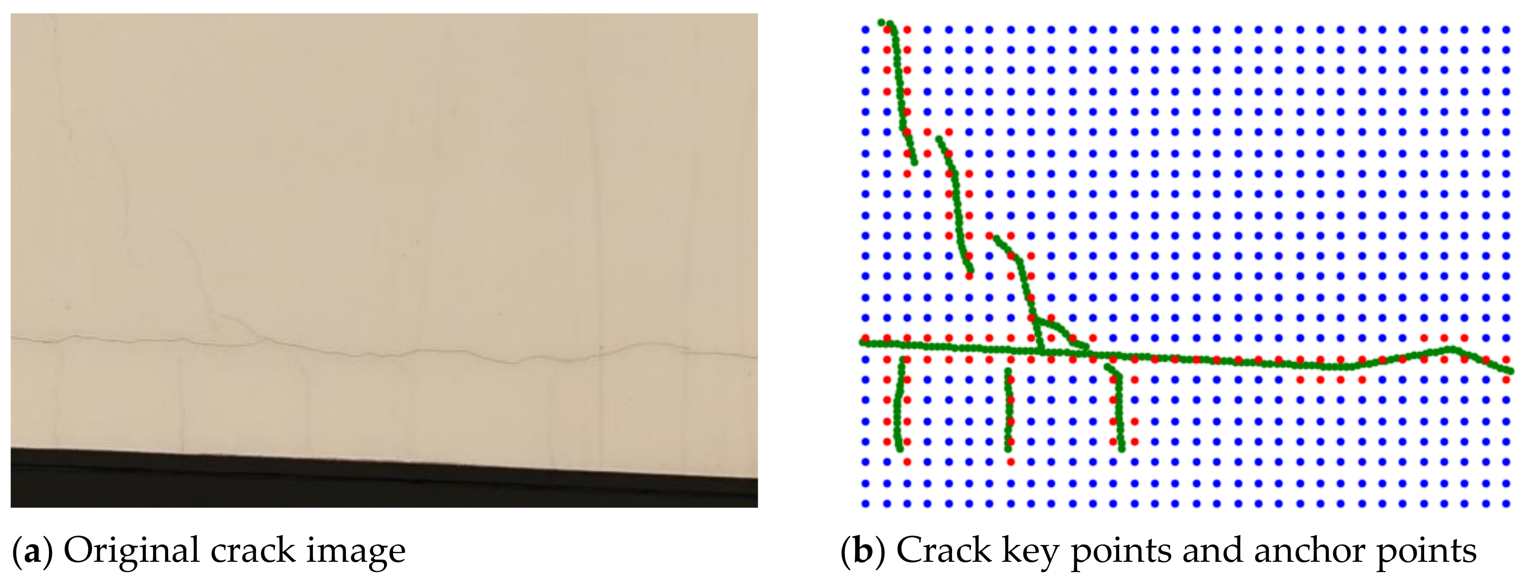
For this purpose, we established a crack detection model that considers the cracks’ linear characteristics and maximizes the use of their global characteristics. Based on the cracks’ linear characteristics, this method can identify cracks as long as the key points on the cracks are identified. Considering the network advantages of traditional computer vision tasks, this research work uses the separation and fusion of the global and local features of cracks to construct a KP-CraNet model for crack detection. Finally, evaluation criteria are set to evaluate the effectiveness and suitability of the model. The numerical experiment has proven that our crack detection model, KP-CraNet, showed a relatively strong detection ability with great potential for further improvement.
3. Crack Detection Model KP-CraNet
To consider the influence on crack detection exerted by the linear and global features of cracks, a crack detection model based on crack key point, KP-CraNet, has been built. The model contains three hierarchical submodels. The bottom submodel is a feature extraction model based on crack key points of deep convolutional neural networks, which is also called a key point feature extraction network or basic network. The second submodel uses feature pyramid fusion and a reinforce network [
38] (FPN feature fusion and reinforce network) to fuse and reinforce the features of extracted key points. The third submodel is a feature filtration network, which filters the features of crack key points, the results of which will lead to an area of a crack key point as an approximate location of a crack.
3.1. The Network Frame of KP-CraNet
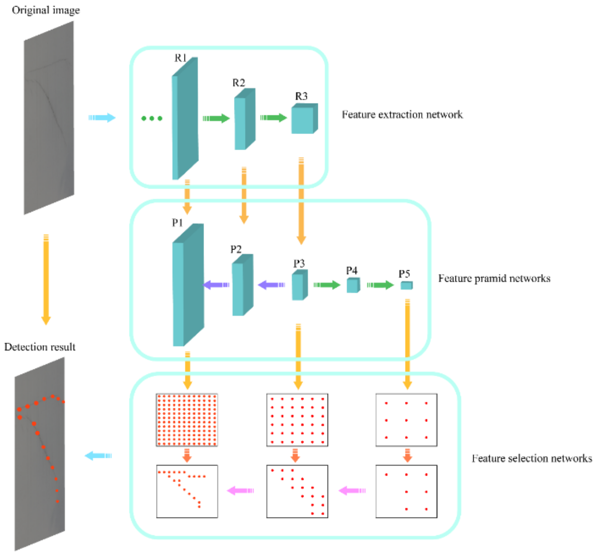
Figure 6 shows the network frame of KP-CraNet. The bottom submodel for crack key point feature extraction adopted the ResNet [
39] network framework, choosing the last three feature layers with different sizes, R1, R2, and R3, as the feature fusion input and reinforce networks. In this network, the FPN reinforcement network is used for global and local feature fusion. The output results are dominated by the current layer features, and the upper layer feature layer is incorporated into the current layer using inverse convolution, outputting a total of five layers. The first three layers have the same size as R1, R2, and R3, while the last two layers are based on the R3 layer, again convolved and downsampled to obtain a smaller layer to better express the global features. Finally, the five feature layers are subjected to feature filtering. The features of feature layers 1, 3, and 5, which are in decreasing size order, are inputted into the feature screening submodel, and the probability of predicting the anchor point as a crack key point is used to screen the positive sample points sequentially to detect cracked and noncracked areas for the final detection of cracks.
3.2. Crack Key Point Feature Extraction Network
The key point feature extraction network uses deep convolutional neural networks, usually adopting ResNet or VGG or other models commonly used in the computer vision field. Crack detection experiments show few differences between the ResNet and VGG models, even when increasing the network depth. Therefore, ResNet18, which requires lower depth, was chosen to decrease the training difficulty and improve the prediction efficiency.
The input to the lowest layer is the image, and the information contained in each pixel of it is the smallest unit of the feature, called the smallest local feature. The topmost layer feature is the crack identification result, and all intermediate result layers from the bottommost to the topmost are called feature layers. For any current layer, whether it is convolution or pooling, the feature points within the range of 3 × 3 convolution kernels or 2 × 2 pooling kernels of the current layer are weighed and summed, and the activation function is used to obtain new information about the feature points. Thus, each feature point of the next layer contains multiple feature point information of the corresponding position of the current layer. The feature information is continuously downscaled and integrated, gradually transitioning from local feature information to global feature information.
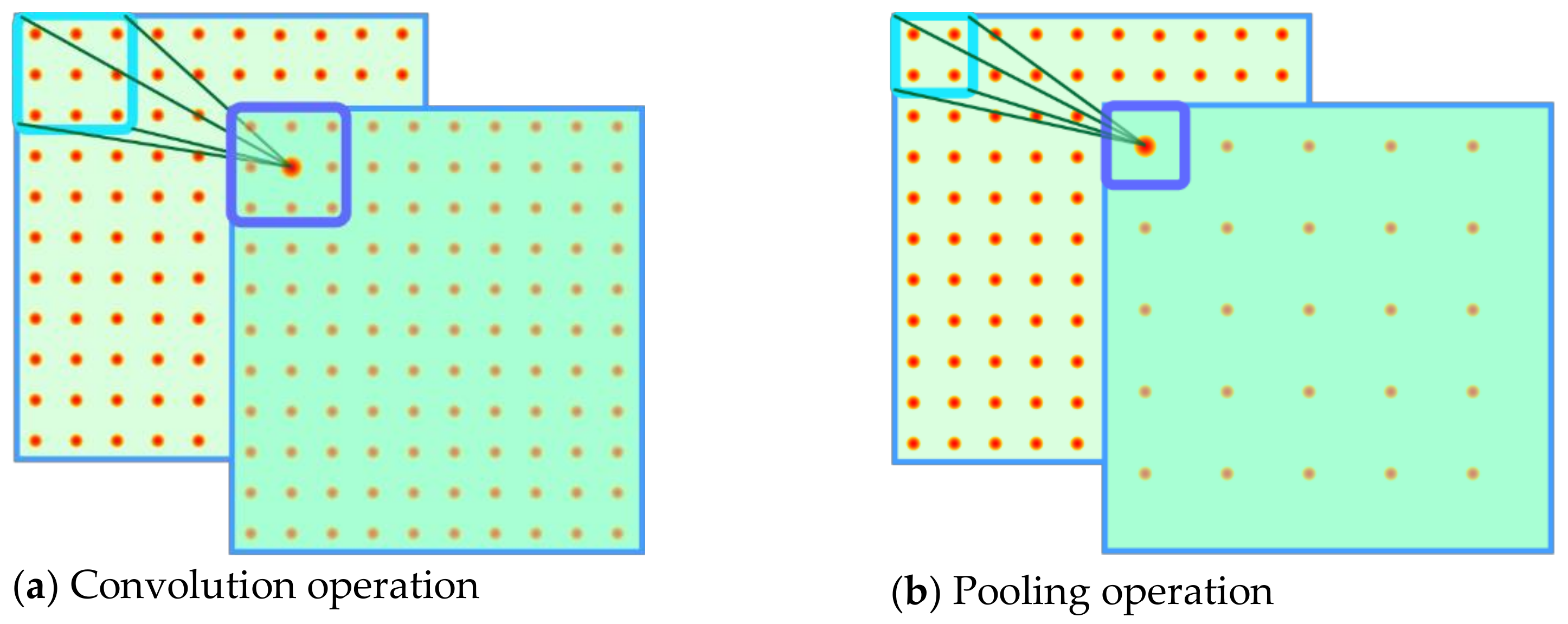
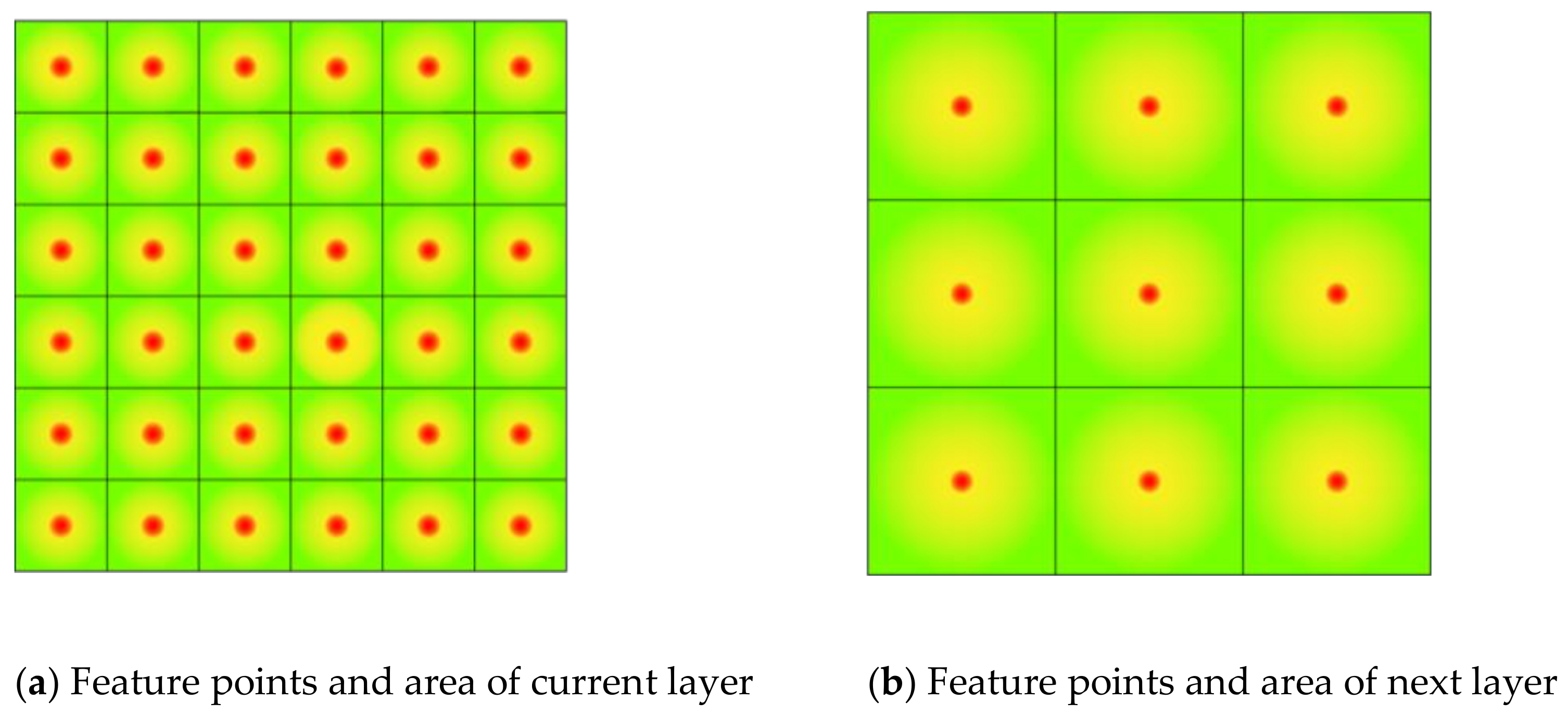
Figure 7a,b shows the convolution and pooling layers. The rear, lighter part is the current layer feature map. The front, darker part is the next layer. The images demonstrate how framed feature points in the current layer descend to the next layer, which means the next layer contains information on points in the current layer, so the local feature information is gradually integrated with the layers, adding up. As the feature layer increases, the area of information contained in feature points becomes larger. The red dots in
Figure 8 are feature points, and the yellow-green background is the feature area. In a higher-level feature map, the feature points reflect global features.
3.3. FPN Feature Fusion and Reinforce Network
Three maps of features from the feature extraction network contain both global and local feature information. Although the specific location of cracks should be precisely positioned by a local feature map, we also need global features as a reference to avoid the errors caused by tree branch shadows and stains that look similar to cracks in pictures. Although, in the feature extraction of single-track networks, higher feature layers contain some of the features of lower layers, the same layers may contain the feature information of different layers in different images because of the varying crack rate. Therefore, it is important to consider both global and local features. Feature information in different layers should be further fused and reinforced to obtain integrated feature information that contains features through all layers. FPN feature fusion and reinforce network is an effective method of feature fusion and reinforces various sizes that are extensively applied in the object detection field. After the convolution and fusion of the three feature maps extracted by the network, three new feature layers are generated, with convolution and pooling operations repeated twice to form a higher global feature layer, so the FPN feature fusion and reinforce network would generate five feature layers in total. Apart from containing more information, it can also process images of different sizes, learn the feature rules automatically, and finally, generate three reinforced feature maps and two with global feature information. We selected the first, third, and fifth layers in sequence as the final extracted feature layer with detailed local features, transition features, and global features.
3.4. Feature Filtration Network
The outputs of FPN feature fusion and reinforce network need another convolution operation for feature processing and finally output an anchor point prediction result the same size as the corresponding original feature layers. Different layers contain different numbers of local or global features, so the prediction results of each layer can be regarded as the prediction results for different features’ extent, i.e., whether the corresponding area contains a crack.
Predictions that consider global features will have higher prediction accuracy, while predictions considering local features will have higher localization accuracy. Thus, starting with global features, the feature points that do not have cracks are gradually filtered out based on the results of the current layer prediction. Finally, the identification results are obtained, and the prediction accuracy and crack location accuracy are guaranteed. The process of crack detection shown in
Figure 9 exemplifies how a feature filtration network works.
Firstly, we input the prediction results of the bottom feature layer that contains the most comprehensive global information, as shown in
Figure 9b, into the feature filtration network. Due to the relatively large distance between feature points, each feature point contains comprehensive global feature information. The prediction result of the current layer helps to distinguish between the crack area and noncrack area, as shown in
Figure 9b. We removed the feature points in noncrack areas and kept those in the crack area, as shown in
Figure 9c.
Based on this filtering result, the feature points corresponding to the next feature layer were retained. As shown in
Figure 9d, the features and anchor points of this layer were screened, and after the screening, only the anchor points of the current layer in the crack-containing area were retained again; this process was repeated continuously. According to the network structure, three times in sequence were filtered, and the points finally retained were the anchor points of the positive sample of the lowest local features at the maximum resolution set and the minimum step size. These were the key points of the identified cracks.
It is important to note that the above method is completely different from directly deciding whether an area contains cracks. The method depends totally on convolution or pooling operations, whose weight is obtained via the model’s automatic learning.
3.5. Feature Filtration Network
In model training, the input for each layer level is the anchor point prediction result of the previous layer of features and the eigenvalue of the current layer of features. The output is the anchor point prediction result of the current layer, which is used to determine whether each anchor point is a positive sample point of the current layer. Due to the different sizes of the input images at different layers, or the different sizes of the feature layers, the tolerance of the critical point determination for identifying cracks is also different. So, the thresholds , , and loss function are determined by the size of feature maps.
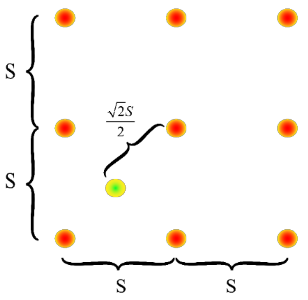
For reticulated reference anchor points at equal intervals, if their anchor point stride is S pixels, then the maximum distance between a crack key point and its nearest anchor point is
pixels. As shown in
Figure 10, the yellow and green points are fracture key points, and the furthest possible location from the nearest anchor point to that fracture key point is the four red points around it.
and
can be extracted to define positive and negative sample anchor points in every layer. When the possibility that the reference anchor point is a positive sample point is higher than the set threshold, the reference anchor points are regarded as positive sample points of the current layer.
A loss function is introduced in each layer to speed up the algorithm convergence and improve the judgment accuracy during training. For this classification problem, a binary cross-entropy loss function can generally be used. However, for image crack detection problems, because a crack occupies only a small part of the whole image, there are many more negative sample points than positive ones, which will lead to error. Therefore, a loss function in RetinaNet [
40] is applied to balance the positive and negative sample points, using the Focal Loss function as in Equation (8):
In order to balance positive and negative samples, regulatory factors α and β were introduced into the formula. is the predicted value, i.e., the possibility that reference anchor points are crack key points of the feature layer. is the actual value of the same reference anchor points: the positive sample point is 1, while the negative one is 0.
4. Model Training and Evaluation
4.1. Data Collection
The dataset used in this research was derived from the surface crack images of various wall surfaces on a university campus in Shanghai. First, we used a camera to take multiple 6720 × 4480 pixel images, divided them into 6 × 6 blocks, and used bilinear interpolation to unify each block image to a size of 1024 × 768. From these images, 1349 images containing cracks were selected; 90% of them were used as the training set and 10% as the test set (
https://github.com/csga11/craData, accessed on 24 November 2021).
4.2. Training Parameters
The crack detection model in this paper was based on the Pytorch 1.0 deep learning framework. The GPU used for training and testing was NVIDIA GTX1080. The initial parameter weights of the feature extraction network all used the weights of the Pytorch official ResNet network pretraining model. During training, the batch size was 16, the number of iterations was 100, and the learning rate was 0.0001. In order to improve the training effect and robustness of the model, conventional online dataset expansion methods, such as random inversion, filtering, and brightness enhancement, were used during the model training.
4.3. Assessment Criteria
The model assessment criteria need to be determined to evaluate whether a crack detection model is effective. For each anchor point, the distance threshold method was applied to determine whether a sample point was positive or negative. As the possibility of positive sample points was calculated as the output, a possibility threshold
had to be set for determining the sample points, i.e., the positive and negative sample point set were as in Equation (9):
where
is the predicted possibility value of the anchor point i.
The commonly used accuracy rate in the object detection area was also adopted to represent the correct prediction rate among all the image detection results as in Equation (10):
In Equation (11), represents the number of elements in the set.
Meanwhile, the introduction of another conventional indicator-recall rate, the proportion of all actual crack points that are correctly identified, describes whether all the key points of the crack are correctly identified. For any key point of a crack, as long as there is an anchor point identified as a positive sample point in the circle whose radius is step S, the key point of the crack is considered to be correctly detected. Therefore, the recall rate was defined as in Equation (11):
It can be seen that, in order to ensure accuracy, forecasts should be as few and precise as possible. However, in order to ensure the recall rate, the prediction should be as complete as possible, so the two indicators are contradictory to a certain extent. According to actual engineering needs, these two parameters can usually be adjusted. Here, the weighted balance F1 score of the two is adopted as the final identification evaluation index. The recall rate is defined as in Equation (12):
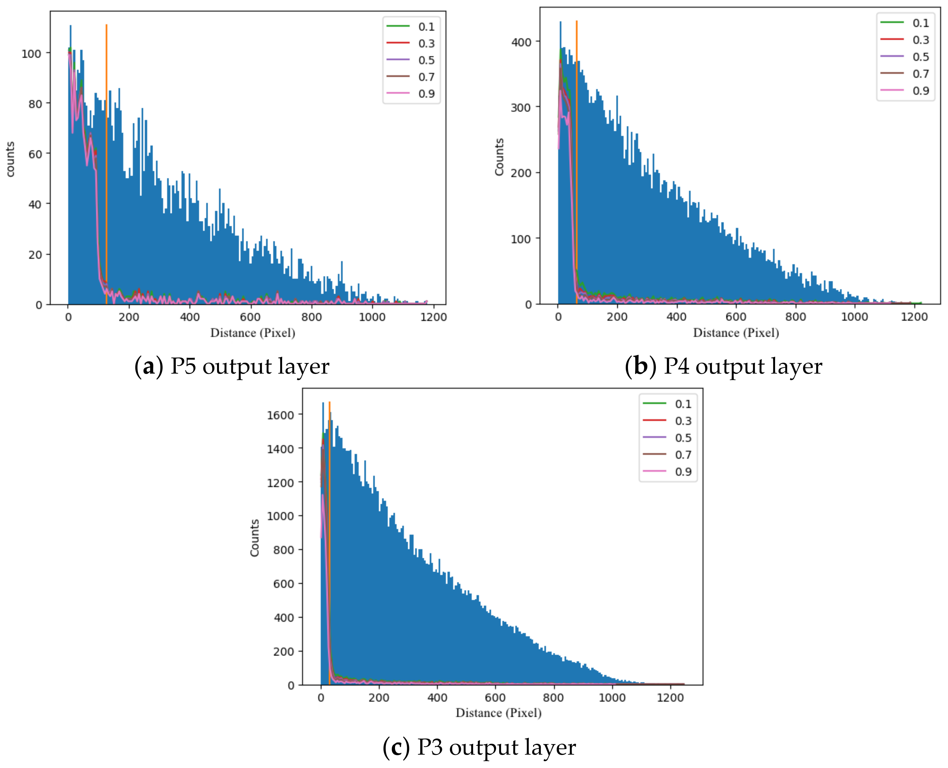
This research proposes the concept of a distance distribution map to reveal the distance distribution of the identification point from the nearest crack key point. The abscissa is the distance between the anchor point and the key point of the nearest crack, and the ordinate is the number of anchor points at the above distance. The results of all the images in the test set were plotted in one graph. The quality of crack detection was evaluated by analyzing the number of anchor points within a certain distance.
4.4. Analysis of Detection
The correctness of the model design needs to be tested first to demonstrate the effectiveness and applicability of the method. We tested three models without a feature filtration subnetwork, then output three layers, P5, P4, and P3. P5 represents the highest layer for global features. After testing the two characteristic screening subnetwork models, P5 is the screening output of P4, and P5 and P4 are the screening output of P3. We set the threshold rate using the experimental results of the above five models, as shown in
Table 1.
When the output layer is a single feature layer, and the sizes of feature layers increase (from P5 to P3), the correctness of prediction gradually drops. The F1 score decreased from 0.895 to 0.831, which showed that the global feature exerted a notable influence on crack detection. So, the global feature should be adequately considered.
However, after adding the feature screening subnetwork, comparing the results of P4 with P5 + P4 and P3 with P5 + P4 + P3 shows that the model has better detection results after adding the feature screening subnetwork. The F1 score increased from 0.853 to 0.862 and from 0.831 to 0.856.
Figure 11 presents a distance distribution map of the detection results of the single-track output layer model. The intensive blue strips are a histogram of the distance between anchor points and the nearest crack key point. This shows that, as the distance between anchor points and the nearest crack key point increases, the number of anchor points reduces. For the orange anchor point segmenting vertical lines in the image, its vertical coordinates are the threshold of positive/negative sample determination for the current feature layer: positive to the left, negative to the right. The curves in different colors are anchor point segmenting lines under different possibility thresholds, and any line divides all the anchor points (blue strips) within the distance into two parts: the upper parts represent the positive prediction points, and the lower represent the negative prediction points. Any point in the curve represents the number of positive points in the corresponding distance, which can be called a positive detection curve.
Any one of the identifying positive case curves and vertical dividing lines divides the blue area into four regions. In the upper left region, the points that are actually positive case anchors are identified as negative case anchors; in the lower left region, the points that are actually positive case anchors are identified as positive case anchors; in the upper right region, the points that are actually negative case anchors are identified as negative case anchors; and in the lower right region, the points that are actually negative case anchors are identified as positive case anchors. The percentage of points in the lower left and upper right areas should be as high as possible.
Therefore, for the P5 output layer shown in
Figure 11a, the positive prediction curves under each possibility threshold almost coincide; the threshold selection has little influence on the result, which means that the global feature exerts a relatively significant influence on model detection and the detection of the crack key point is accurate. The prediction rate of anchor points marked as positive is close to 1, while the prediction rate of anchor points marked as negative is close to 0, which is an ideal prediction result.
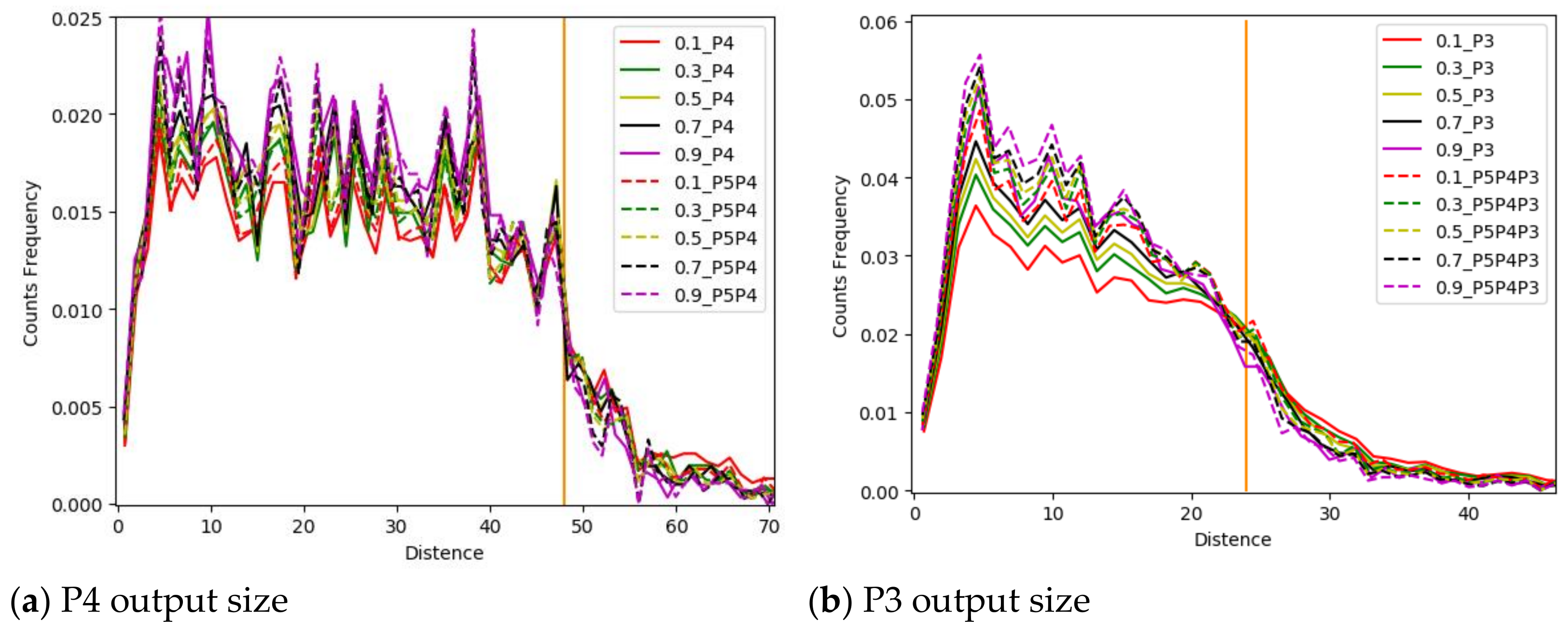
Figure 11b,c demonstrate that, with the decrease in stride, the detection result of the positive/negative sample point becomes more sensitive to the possibility threshold, and more detection errors appear, because images with high resolution emphasize the local features, leading to the misjudgment of anchor points in areas such as cracks. This illustrates that global features are more helpful for effective crack detection, yet the relatively long stride complicated the accurate location of cracks. The introduction of a filtration subnetwork requires a correction of the distance distribution map, because the number of anchor points is influenced by the feature filtration subnetwork and the size of its output. Changing the vertical ordinate from the number of anchor points to the anchor point frequency would reduce the influence of the model anchor point to an extent.
Figure 12 presents the distance distribution map of a single-track output layer and introduces the feature filtration layer under a different possibility threshold. It shows that the curves become steep near the possibility threshold after introducing the feature filtration network, especially the output of P3; more points are detected near the crack key points, and fewer are detected away from the crack key points. The figure illustrates that the feature filtration network has a significant effect, verifying the suitability of the networks we presented.
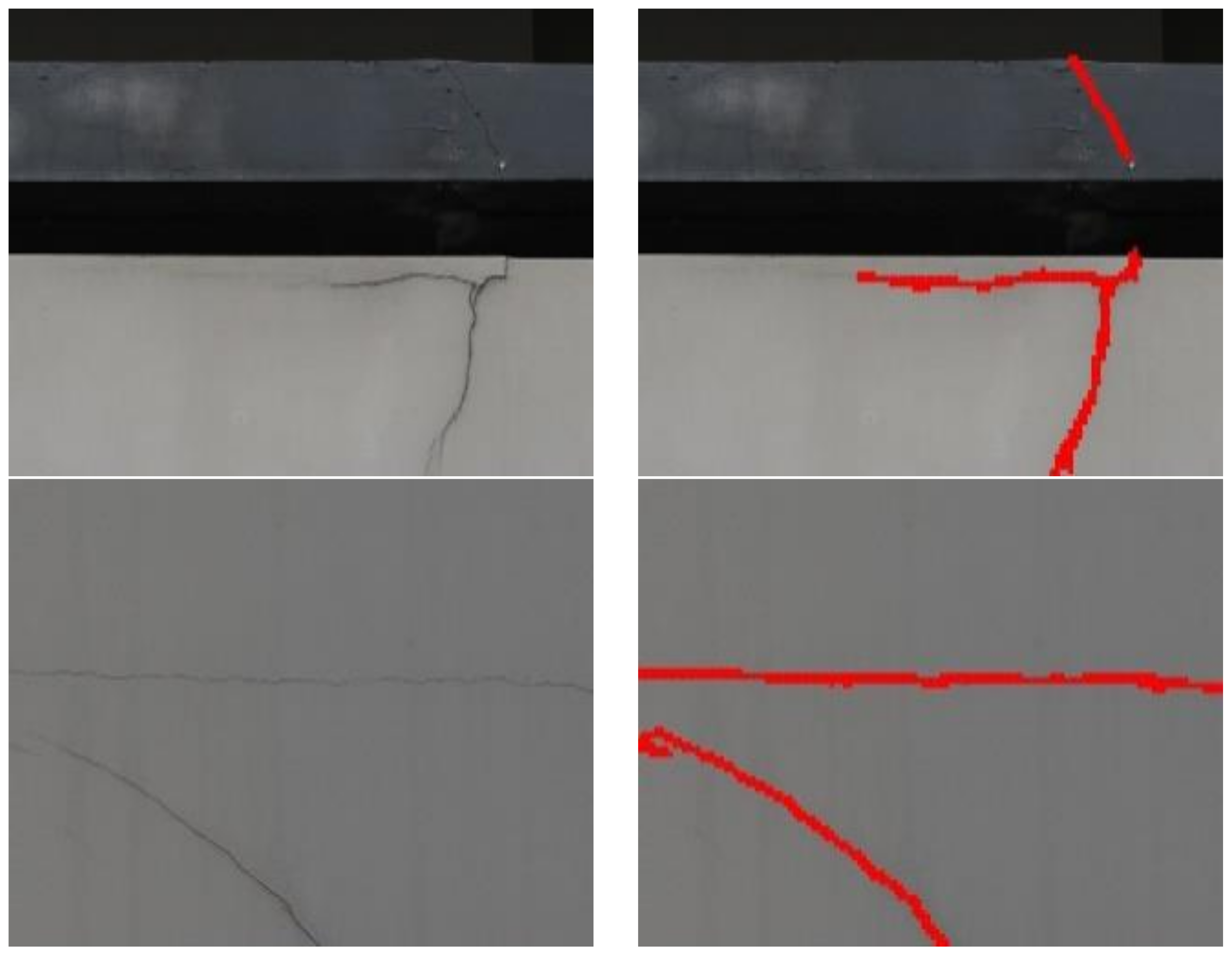
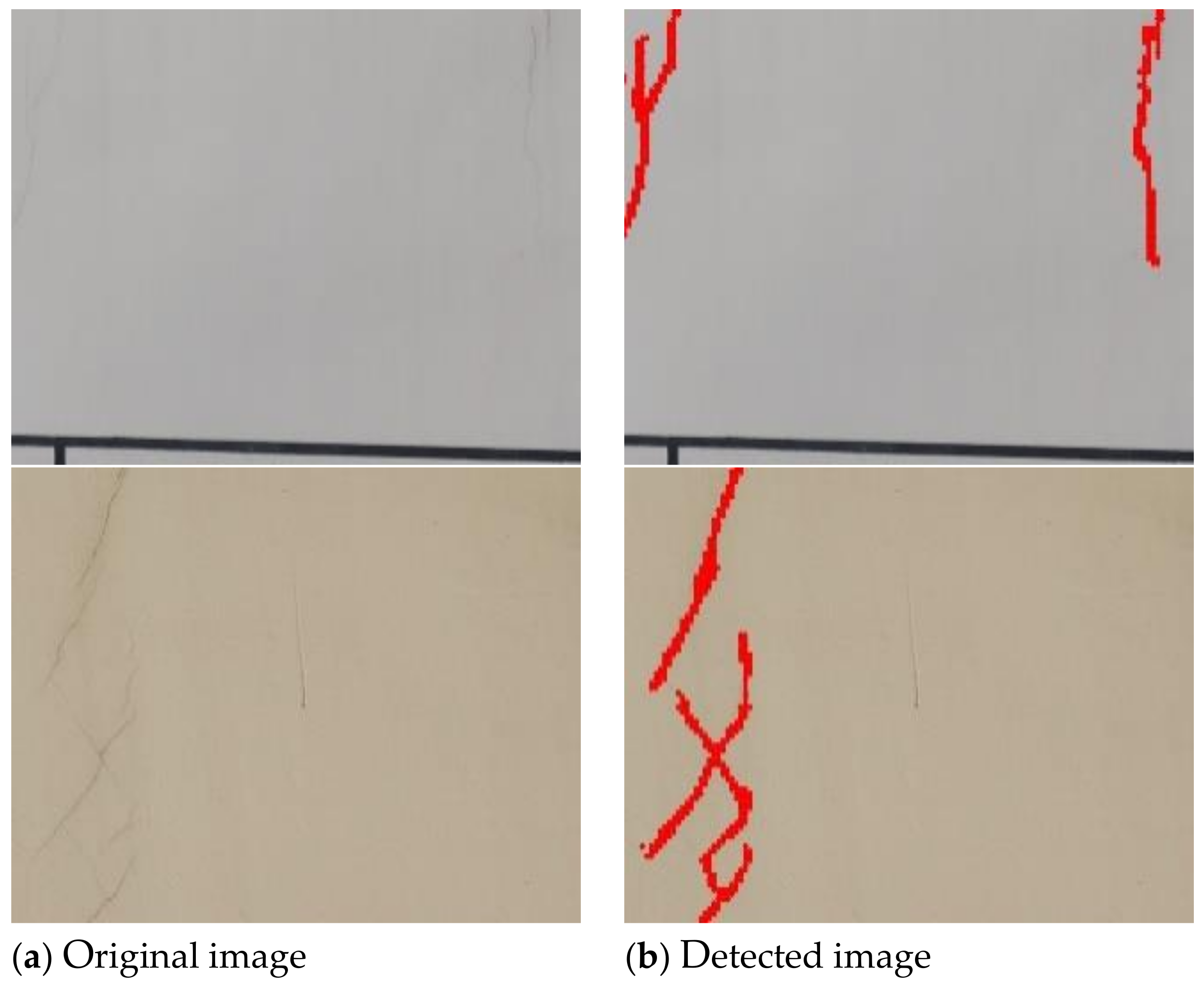
Finally, we chose P5 and P3 as feature filtration layers, while P1 was an output layer. The final results of different crack detection were as shown in
Figure 13. This figure proves that the application of our detection model can lead to satisfactory crack detection results. Moreover, the detection experiments discovered that the model had good generalizability, enabling the model to detect manual marking errors.
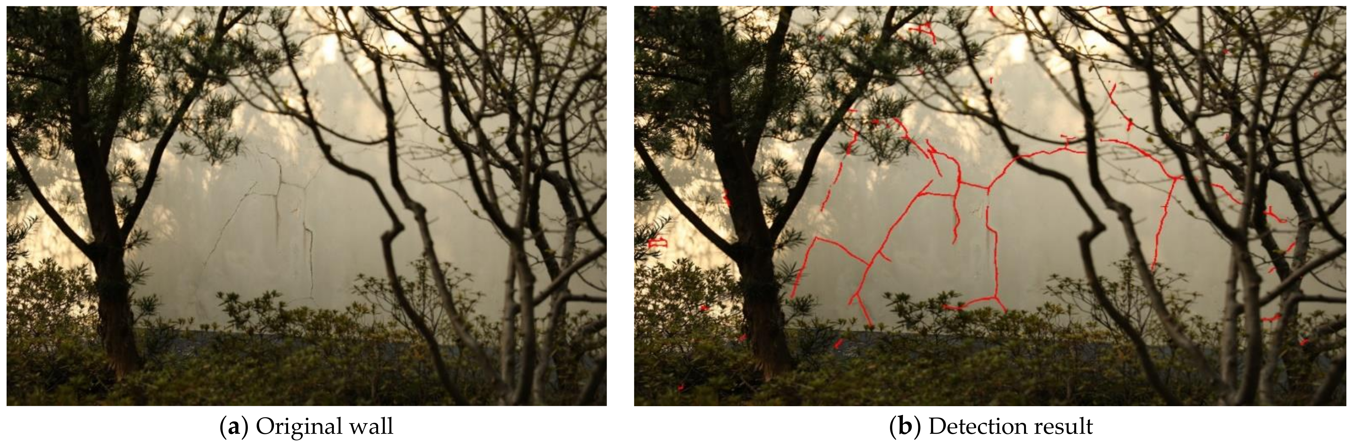
Figure 14a was used to identify cracks.
Figure 14a contains much interference, such as cracks, shadows, and numerical values. The model detection result is shown in
Figure 14b. The comparison of the two figures shows that the model can detect cracks in a complex environment and meets the basic requirements of crack identification in a practical engineering environment. The suitability of the model design proposed in this research has been verified again. It is worth mentioning that the method proposed in this paper utilizes points but not crack characteristics in the marking stage. Therefore, width recognition of cracks is not accurate enough. We should consider modifying and optimizing this method in future research.


