SAEP: A Surrounding-Aware Individual Emotion Prediction Model Combined with T-LSTM and Memory Attention Mechanism

Abstract

The future emotion prediction of users on social media has been attracting increasing attention from academics. Previous studies on predicting future emotion have focused on the characteristics of individuals’ emotion changes; however, the role of the individual’s neighbors has not yet been thoroughly researched. To fill this gap, a surrounding-aware individual emotion prediction model (SAEP) based on a deep encoder–decoder architecture is proposed to predict individuals’ future emotions. In particular, two memory-based attention networks are constructed: The time-evolving attention network and the surrounding attention network to extract the features of the emotional changes of users and neighbors, respectively. Then, these features are incorporated into the emotion prediction task. In addition, a novel variant LSTM is introduced as the encoder of the proposed model, which can effectively extract complex patterns of users’ emotional changes from irregular time series. Extensive experimental results show that the proposed approach outperforms five alternative methods. The SAEP approach has improved by approximately 4.21–14.84% micro F1 on a dataset built from Twitter and 7.30–13.41% on a dataset built from Microblog. Further analyses validate the effectiveness of the proposed time-evolving context and surrounding context, as well as the factors that may affect the prediction results.

1. Introduction

Emotions affect the status of humans physiologically and psychologically. One may make a quick decision simply because of a particular feeling. Nowadays, more and more people are used to sharing their emotions and opinions through texts on social networks. It is interesting to understand how an individual’s emotions are affected by various factors and predict his future emotion.

Individual emotion prediction aims to determine the future emotional state of a user from current and previous behavioral cues [1] and has potential applications in various fields, such as human–computer or human–robot interactions [2], market analysis [3], public opinion analysis [4], political decision-making [5], and recommendation systems [6]. In recent years, several researchers have conducted research on individual emotion prediction by using texts of users’ posts and comments.

For emotion prediction, most traditional methods use statistical models and machine learning methods. However, these methods, which are limited to binary classification, have poor performance and low effects. In recent years, deep learning has addressed the limitations of traditional approaches, which predict and classify individual emotions by modeling the time series of users’ emotions. However, existing deep learning models are relatively simple. Most of them mainly rely on the user’s own emotional development rules, while ignoring the neighbors’ effect on the user’s emotion. In fact, the way in which users share their emotions online affects not only their own emotions [7], but also the emotions of others with whom they relate [8]. Furthermore, Bond et al. [9] find that strong ties are instrumental in spreading individual emotions both in the online and practical world.

In addition, users’ posts and comments in adjacent time periods are interrelated, and it is necessary to consider the relevance and dependence between users’ posts when predicting their personal emotions. However, users optionally publish their posts and comments on social networks. Irregular time series data are common in social networks [10]. Thus, it is challenging for the individual emotion prediction task to use the time series data of user posts and comments.

This study focuses on the problem of individual’s future emotion prediction in the context of irregular time series. The problem setup is illustrated in Figure 1. Given a social network in which each vertex (A, B, C, D) represents a user, there is an undirected edge between two users if they have a social network relationship. The users’ emotion data (from users’ posts and comments) are classified into three types. It includes the observed data (green boxes and circles), missing data (red boxes and circles), and goal data (purple boxes and circles). Every user’s emotion is represented by a six-dimensional vector, composed of the probability of six basic emotion categories (i.e., happiness, sadness, anger, disgust, fear, and surprise) proposed by [11]. The goal of this paper is to predict the emotions of users A and D at timestamp 3. To predict user A’s emotion at timestamp 3, the traditional methods utilize A’s previous emotion data at timestamps 1 and 2. However, in both timestamps 1 and 2, A’s previous emotion data were missing. Interestingly, neighbors’ (users B and C) emotion data can provide clues for predicting user A’s emotions. For instance, as the number of user A’s neighbors with happy emotions increases, the probability that the user will be happy continues to increase. It turns out that happy users influence other users to feel happy as well, which means that emotions spread through social networks [12]. These relationships are refered as the surrounding influence. The first challenge is to capture this surrounding influence and model the connection between the user’s future emotion and the surrounding influence.

Returning to Figure 1, user D’s emotion also needs to be predicted. In addition to receiving the surrounding influence, the emotion of user D at timestamp 3 is affected by D’s emotion at timestamp 1 (due to the absence of the emotion of user D’s emotion at timestamp 2). These relationships are defined as time-evolving influence. In this study, the second challenge is extracting the time-evolving influence in irregular emotion time series.

To address the aforementioned challenges in individual emotion prediction, a surrounding-aware individual emotion prediction model (SAEP) is proposed, which is based on a deep encoder–decoder architecture, adopts an attention mechanism to combine the surrounding influence and time-evolving influence into the emotion prediction task. Specifically, SAEP constructs two attention networks: A time-evolving attention network and a surrounding attention network. The time-evolving attention network extracts the time-evolving context from the user’s emotion time series. The surrounding attention network obtains the surrounding context from the emotion time series of neighbors. Next, the time-evolving influence and surrounding influence are integrated to predict the user’s future emotion. Following are the main contributions of this study:

• Based on a deep encoder–decoder architecture, a surrounding-aware model is proposed to predict individual emotions in social networks, which takes into account both the influences of time-evolving and social network surrounding. First, the time-evolving and surrounding attention networks are constructed. Then, two attention context vectors are incorporated, time-evolving information and surrounding information, into the emotion prediction task.
• Aiming at the problem of irregular time series data, a variant long short-term memory (LSTM) network is introduced as the encoder of the proposed model, to extract the underlying structure in irregular time series data, allowing it to capture individual emotional changes more precisely. To the best of the authors knowledge, there is a lack of research on emotion prediction for irregular time series data based on surrounding influence and deep learning techniques.
• Extensive experiments were conducted to validate the proposed model over several baseline methods. The experimental results show that the micro F1 of SAEP can reach 60.20% and 63.33% on Twitter and Microblog datasets, respectively.

2. Related Work

2.1. Emotion Classification

Emotion classification aims to classify the sentiment polarity of a given text as positive, negative, or more fine-grained classes. Early studies on predicting emotion simply classify individual emotions as positive and negative, or just a score of well-being. With the help of emotional research, people find that more fine-grained emotions are of great significance in many fields. Ekman [11] propose six basic emotions, including happiness, sadness, anger, disgust, fear, and surprise.

In the past, emotion classification research mainly relied on high-quality emotional dictionaries. Keshavarz and Abadeh [13] combine corpora-based and lexicon-based methods to build adaptive emotion lexicons to improve the performance of emotion classification. Chekima and Alfred [14] utilize existing emotion analysis resources and tools from English along with the automated machine translation capability to automatically build a Malay emotional dictionary.

The development of machine learning has led to its gradual application to the analysis of textual emotion. Song et al. [15] use a naive bayes model to classify emotions in text, which reflects the difference of the number of positive words and negative words in calculating the weights. Liu et al. [16] provide a method for multiclass emotion classification based on an improved one-vs-one strategy, and use a support vector machine (SVM) model to classify emotion. Xie et al. [17] represent a maximum entropy model, which uses the probabilistic latent semantic analysis to extract emotional features from corpus.

Inspired by the recent success of attention-based neural networks in natural language processing, various neural network approaches have been proposed for emotion classification [18]. Wang et al. [19] propose an attention-based LSTM method to learn an aspect embedding for each aspect and made aspects participate in computing attention weights. Wang et al. [20] propose a convolutional recurrent neural network for text classification for emotion classification, which combines convolutional neural network with recurrent neural network.

2.2. Emotion Prediction

The traditional analysis of individual emotion focuses on mining individual emotions at a given time point. In contrast, the present research focuses on predicting individual emotions at some time in the future. Recently, the mining of individual emotions has attracted increasing interest. Individual emotion prediction is a new research direction, with few related citations.

Statistical methods, such as SVM and deep learning have been popular for emotion prediction [21]. Many studies have adopted different machine learning algorithms to predict a user’s emotions at the next moment. Borg and Boldt [22] adopt the linear SVM algorithm to predict the emotion of an e-mail one step ahead in the thread (based on the text in the an already sent e-mail), and the results indicate a predictable pattern in e-mail conversation that enables predicting the emotion of a not-yet-seen e-mail. Adikari et al. [23] utilize Markov chains and growing self-organizing maps to construct a comprehensive framework based on the principles of self-structuring artificial intelligence for emotion modeling. Zhang et al. [24] propose a factor graph-based emotion prediction model to predict emotions by combining emotion labels correlations, social correlations, and temporal correlations from dataset.

With the development of deep learning technology, approaches based on time series prediction have been further developed. Several studies have demonstrated the strength of deep neural networks in solving time series prediction problems [25,26]. It has also been applied to emotion-prediction tasks. Majumder et al. [27] propose a method based on recurrent neural networks (RNNs) [28], which employ three gated recurrent units (GRU) [29] to model three key aspect in the textual dialogue, thereby extracting emotional features for emotion prediction. Zhang et al. [30] design a variational learning network, which infers an appropriate emotion label based on both the dialogue context and the learned latent distribution in continuous semantic space. Lubis et al. [31] propose a hierarchical neural dialogue system with an emotion encoder to capture the emotional context of the dialogue. This information is then used in the response generation process to produce an affect-sensitive response that elicits positive emotion. Liu et al. [32] feed the semantic vector of each word with its affective vector together into the conditional variational auto-encoder model, enabling the model to learn the response’s affective distributions, thereby predict an appropriate emotion for response generation. Li et al. [33] propose a fully data-driven interactive double states emotion cell model (IDS-ECM), which has two layers. The first layer extracts the emotional features of the textual dialog, and the second layer models the change process of users’ emotions during the dialog. Tang et al. [34] propose a joint framework for emotion prediction and emotion-reason extraction by introducing a multi-level attention module and bidirectional encoder representation from transformers (BERT) [35] enhanced encoder. Sun et al. [36] adopt the emotion dictionary to predict which emotion in the dialogue, and combine reinforcement learning with emotional editing constraints to generate more meaningful emotional replies. Huang et al. [37] introduce a novel reinforcement learning network, which keeps track of the gradual emotional changes from every utterance throughout the dialogue for each utterance’s emotion detection. Ma et al. [38] represent a hierarchical attention network with residual gated recurrent unit framework for emotion prediction in conversation. Li et al. [39] propose a fast, compact and parameter-efficient party-ignorant framework named bidirectional emotional recurrent unit for conversational emotion prediction, which consists of a generalized neural tensor block and a two-channel classifier.

Despite the success of these methods, most focus on the information of the user’s emotion changing process and ignore the influence of neighbors on the user’s future emotion. In addition, many approaches require data with high continuity and integrity without the analysis of the common irregular time series of the social network platform. Therefore, in this paper, a surrounding-aware individual emotion prediction model is proposed that combines the surrounding influence and time-evolving influence with the memory-based attention mechanism and considers the irregular emotion time series.

3. Preliminaries

This section briefly describes key definitions and some notational conventions to simplify the elaboration of the following sections to help readers better understand the design ideas of the proposed model.

Notations and Definitions

Emotion Vector: Emotion vector is designed to quantify an individual’s emotion. In this study, six basic emotion categories [11] are used to express compound emotions. An individual’s emotional state is represented by using a 6-dimensional vector as follows:

$$S=\{s_{happy},s_{sadness},s_{anger},s_{surprise},s_{fear},s_{disgust}\}.$$

(1)

where $s_d$ denotes the probability of the d-th basic emotion category and it is intermediate value within the range $[0,1]$. For example, $s_1$ denotes the happiness score of the emotion vector.

Social Network: A social network represented as an undirected graph $G=\{V,E\}$, where $V=\{v_1,v_2,\cdots ,v_n\}$ is a collection of users, and $E\subseteq V\times V$ is the set of edges whose element $e_{ij}=(v_i,v_j)$ indicates that user $v_i$ and user $v_j$ are friends in the social network.

Emotion Time Series: Emotion time series depicts the process of an individual’s emotion changes in a period of time. Given a user $v_i$, their emotion time series are defined as $X=\{x_1,x_2,\cdots ,x_T\}\in {\mathbb{R}}^{T\times \left|S\right|}$, where $\left|S\right|$ is the dimension of the emotion vector. For each time stamp $t\in \{1,2,\cdots ,T\}$, $x_t$ represents the emotion vector of user $v_i$ at time stamp t.

Masking Series: Masking series marks valid data in emotion time series. A user $v_i$’s masking series is represented as $M=\{m_1,m_2,\cdots ,m_T\}$, where $m_t=0$ if the value of $x_t$ is missing; otherwise, $m_t=1$.

Observed Series: Observed series is composed of the valid values in the emotion time series. For each user $v_i$, the valid values are extracted from the emotion time series and concatenated to construct the observed series $X^{{}^{\prime }}=\{x_1^{{}^{\prime }},x_2^{{}^{\prime }},\cdots ,x_u^{{}^{\prime }}\}$, where u denotes the number of valid emotion vectors in the emotion time series.

Time Interval Series: Time interval series represents the elapsed time between adjacent valid values in the emotion time series. For each user $v_i$, the time interval series is defined as $\Delta T=\{\Delta t_1,\Delta t_2,\cdots ,\Delta t_u\}$, where u is the number of valid emotion vectors in the emotion time series. The time interval $\Delta t_u$ is calculated as follows:

$$\Delta t_u=\left\{\begin{array}{cc}1,\hfill & \hfill u=1\\ t_u-t_{u-1},\hfill & \hfill u\ne 1\end{array}\right.$$

(2)

where $t_u$ represents the timestamp of u-th valid emotion vector.

An example of the emotion time series X, observed series $X^{{}^{\prime }}$, masking series M, and time interval series $\Delta T$ is shown in Figure 2.

4. Observations

Before describing the proposed model for predicting individual future emotions, a data-driven method was used to conduct a series of analyses on the trend of individual emotions in social networks, and validate that the individual emotions are affected by time-evolving as well as surrounding influences.

For individual emotional states, the proposed model considers Ekman’s six emotions [11]. The evolution of individual emotions over time and the influence of neighbors’ emotions are two crucial factors. To determine the relationships between temporal evolution, surrounding influence, and individual emotions in online social networks, this paper focuses on the following two aspects:

• The association of individual emotional states in the adjacent times, including the continuity of the same individual emotions and the transference of different emotions.
• When neighbors share their individual emotions, these individual emotions influence the other’s individual emotions in social networks.

The Microblog dataset used here represents the posts and emotions of 4474 users from January to April 2018. (See Section 6.1 for more details on the dataset).

4.1. Time-Evolving Influence Observation

This subsection aims to explore the correlation between the user’s emotional states at two adjacent times. Tang et al. [40] used a mobile network dataset to quantify the individual emotional states, and their work showed that there is a strong dependency between one’s current emotional state and her emotional state in the recent past. However, their findings were based on emotion polarity analysis. The proposed model focuses on more fine-grained emotions.

An individual emotional state transition matrix (Figure 3) was obtained by analyzing the users’ individual emotional changes on the Microblog social network, which confirms the temporal correlations of the individual emotional states on the Microblog dataset. As the individual emotional state transition matrix is shown in Figure 3, the element in the i-th row and j-th column represents the conditional probability that the user’s individual emotion at time $t-1$ is x and that at time t is y.

As shown in Figure 3, when a user feels happy at time $t-1$, the probability that he feel happy at time t is 60%. For some negative emotions, such as sadness and anger, users in the Microblog social network tend to overcome their negative emotions in the next moment. This causes the adjustment of users’ subjective psychology. In addition, when users feel disgusted at time $t-1$, they are more likely to stay in the same emotional state at the next time t, and the probability that users will feel happiness is only 35%.

Figure 3 illustrates that the users’ future emotions are strongly dependent on their past emotions. When a user feels happiness, they are more likely to continue to feel happiness than others. This confirms the temporal inheritance of the emotional states in social networks.

4.2. Surrounding Influence Observation

With the prevalence of online social networks, users can easily share emotions and influence each other. This subsection aims to explore the correlation between neighbors’ emotions and their impact on the user’s individual emotion. Specifically, users’ historical posts on the Microblog social network are mined. Then, their emotions in terms of what they share are analyzed. Futhermore, given a user v, when the emotion of the user’s neighbors at time $t-1$ is e, the probability that the user’s emotion is e at time t is computed. The results are shown in Figure 4.

As illustrated in Figure 4, as the number of happy neighbors increases, so does the probability that the user will be happy. This means that the user’s emotions are affected by their neighbors. Moreover, there is an interesting pattern about emotion contagion, where a user tends to become more negative when a friend or two is in negative emotion (e.g., fear, sadness). However, when the number of negative neighbors is more than three, the probability of the user being negative decreases significantly. This phenomenon is called “soothing” [41]. When neighbors are depressed, they comfort each other to adjust their negative emotions.

To briefly summarize, this paper have the following intuitions:

• One’s future individual emotional states are related to their past individual emotional states.
• One’s future individual emotional states are influenced by their neighbor individual emotional states.

5. Surrounding-Aware Individual Emotion Prediction Model

5.1. Architecture

The proposed model aims to predict individuals’ emotions in the future for a given social network. Figure 5 shows the basic process of the proposed model. As shown in Figure 5, the proposed model consists of two main modules: A time-evolving attention network and a surrounding attention network.

In a time-evolving attention network, the time-aware LSTM (T-LSTM) is used to extract the memory representation from the user’s emotion time series, and then use the current hidden state of the LSTM encoder with the memory representation to generate the time-evolving context. In the surrounding attention network, a T-LSTM network is also used to extract the fixed-size memory representations of the neighbors and obtain the surrounding context by concatenating them with the current hidden state of the LSTM encoder. Finally, the time-evolving context and the surrounding context are concatenated to predict the target user’s future individual emotion in the fully connected layer and softmax layer.

5.2. T-LSTM Network

LSTM [42] was designed to capture long- and short-term dependencies while overcoming the vanishing gradient problem. However, a standard LSTM network implicitly assumes that the time intervals between the elements of an input sequence are the same, which means that LSTM has difficulty in handling irregular time series data with missing values.

In recent years, to use LSTM network to capture information in irregular series data, more innovative solutions have been proposed [43]. One method involves imputing data to make the time intervals between the elements of the input sequence to be regular. Based on this idea, many studies have estimated missing data by treating imputed values as trainable variables. However, the limitation of this method lies in the fact that the estimated missing data are evidently different from reality.

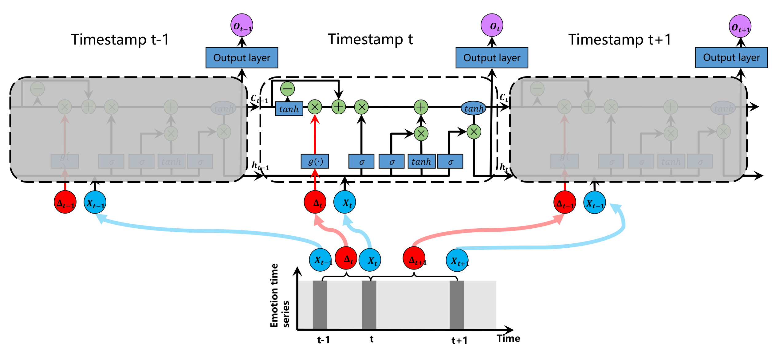
Another method to solve the time irregularity is to adjust the memory unit of LSTM by using the short-term memory discount. This method of using time gaps to adjust memory is called T-LSTM [44]. The T-LSTM architecture is presented in Figure 6. Blue boxes denote networks, and green circles indicate point-wise operators. T-LSTM takes time series and time intervals as input. The major component of the T-LSTM architecture is the subspace decomposition applied to the memory of the previous time stamp, which decomposes the previous memory into long-term and short-term components, and uses the time interval (${\Delta }_t$) to discount the short-term influences.

First, using the memory of the previous moment, the short-term memory is obtained through the network. Note that this decomposition operation is data-driven, and its parameters are learned at the same time as the rest of the network parameters by back-propagation. After the short-term memory $c_t^s$ is computed, considering that the effect of short-term memory is also related to the time gap, a time decay function $g(\Delta t)$ is used to calculate the weight and adjust short-term memory to obtain the discounted short-term memory ${\overline{c}}_t^s$. Finally, to compose the adjusted previous memory back $c_{t-1}^{*}$, the complement subspace of the long-term memory $c_{t-1}^L$ is combined with the discounted short-term memory. The detailed mathematical expressions of the T-LSTM network in Figure 6 are given by Equations (3)–(8) [44].

$$c_{t-1}^s=tanh(W_d{c}_{t-1}+b_d)$$

(3)

$${\overline{c}}_t^s=c_{t-1}^s·g(\Delta t)$$

(4)

$$c_{t-1}^L=c_{t-1}+c_{t-1}^s$$

(5)

$$c_{t-1}^{*}=c_{t-1}^L+{\overline{c}}_{t-1}^s$$

(6)

$$\overline{c}=tanh(W_c{x}_t+U_c{h}_{t-1}+b_c)$$

(7)

$$c_t=f_t·c_{t-1}^{*}+i_t·\overline{c}$$

(8)

where $h_{t-1}$ is the previous hidden state. $c_t$ and $c_{t-1}$ represent the current and previous cell states, respectively. $\Delta t$ is the time interval, and $g(·)$ is a heuristic decay function, so the larger the value of $\Delta t$, the less the effect of short-term memory. Different types of $g(·)$ can be chosen according to the application requirements. For example, $g(\Delta t)=1/\Delta t$ is preferred for less time-consuming datasets, and $g(\Delta t)=1/log(\Delta t+e)$ can be selected for more time-consuming datasets. After the experimental analysis, a better performance of $g(\Delta t)=1/\Delta t$ is used in the proposed SAEP model.

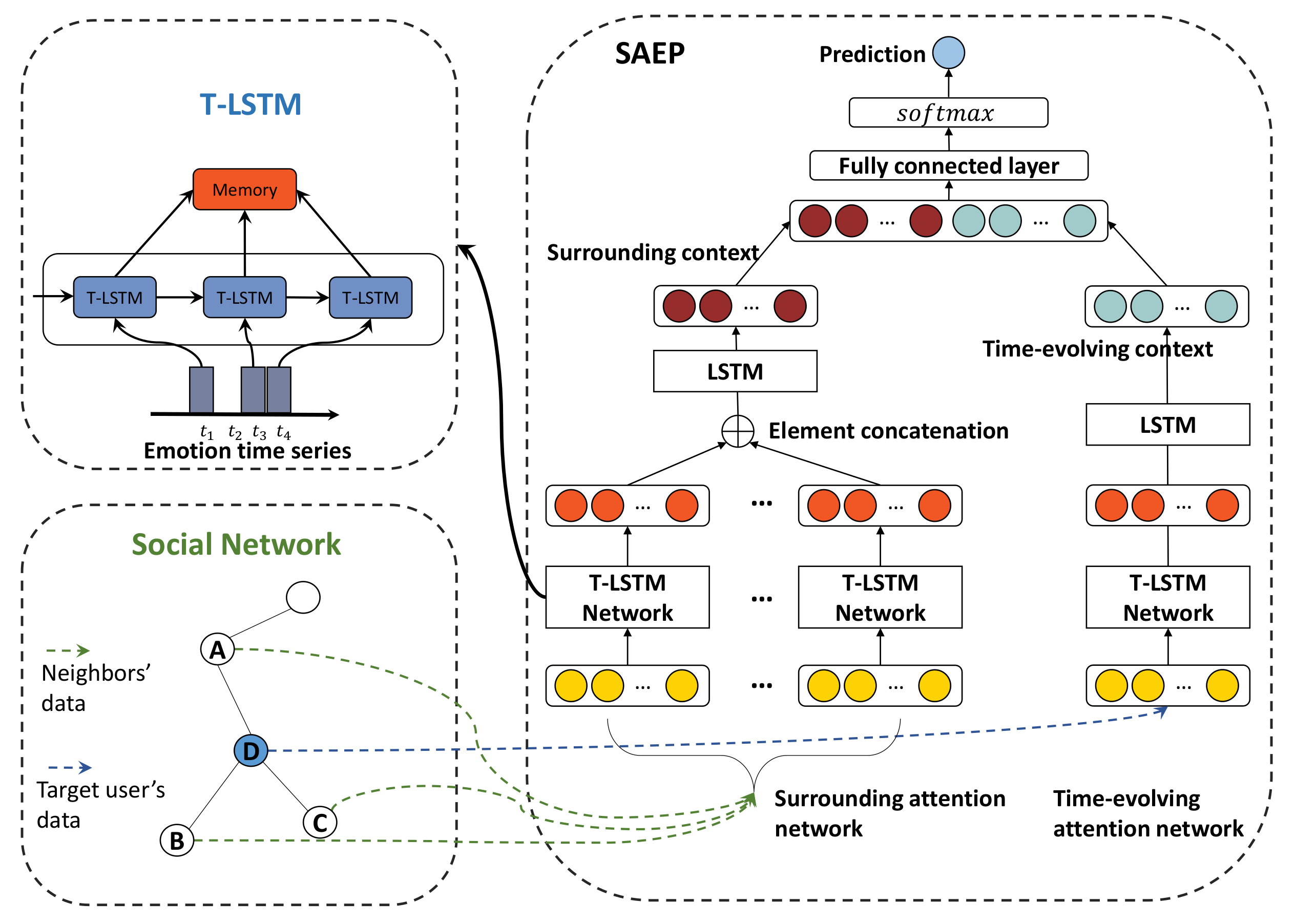
5.3. Time-Evolving Attention Network

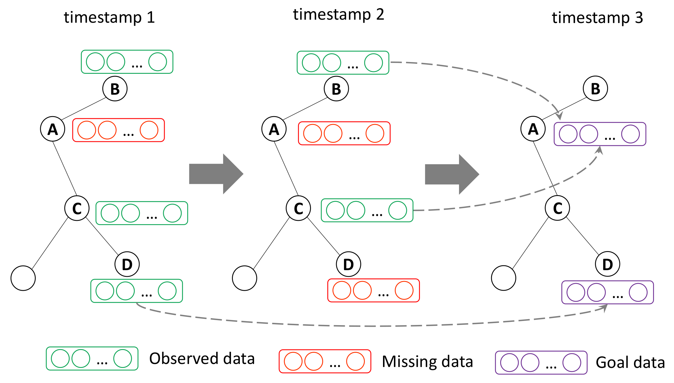
An important factor that should be considered for individual emotion prediction is the time-evolving influence, that is, how a user’s historical behaviors and individual emotional states can be related to the individual future emotional states. To capture this temporal correlation of users’ emotional states, a memory-based attention network is constructed in the proposed model, called time-evolving attention network.

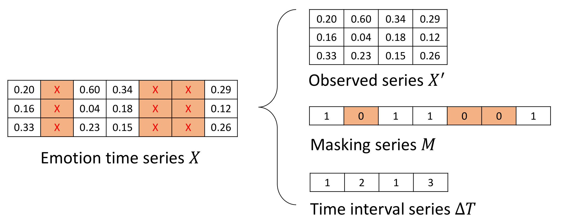
Given a user $v_i$, their emotion time series X is used to extract the observed series $X^{{}^{\prime }}$ and time interval series $\Delta T$. In the encoding phase, the goal is to use a T-LSTM network to capture information in an irregular time series. A T-LSTM network is used to encode the information of the user’s individual emotional change trend in the form of a T-LSTM hidden state, which takes the observed series $X^{{}^{\prime }}$ and time interval series $\Delta T$ as input data. The iterative process is expressed by Equation (9).

$$h_u,c_u=T-LSTM(x_u^{{}^{\prime }},\Delta t_u,h_{u-1},c_{u-1})$$

(9)

where $c_u$ and $h_u$ respectively are cell adjusted state and hidden state.

Many approaches capture contextual information in a time series. The most popular method is based on the encoder–decoder architecture consisting of two RNNs and an attention mechanism that aligns the target to the source tokens [45]. The attention mechanism used in these methods calculates the attention context by analyzing the encoder and decoder at each step. However, such calculations are expensive. Britz et al. [46] present a memory-based attention approach, and they demonstrate the efficiency of their model in experiments. In this paper, a memory-based attention approach is used to efficiently compute the time-evolving context.

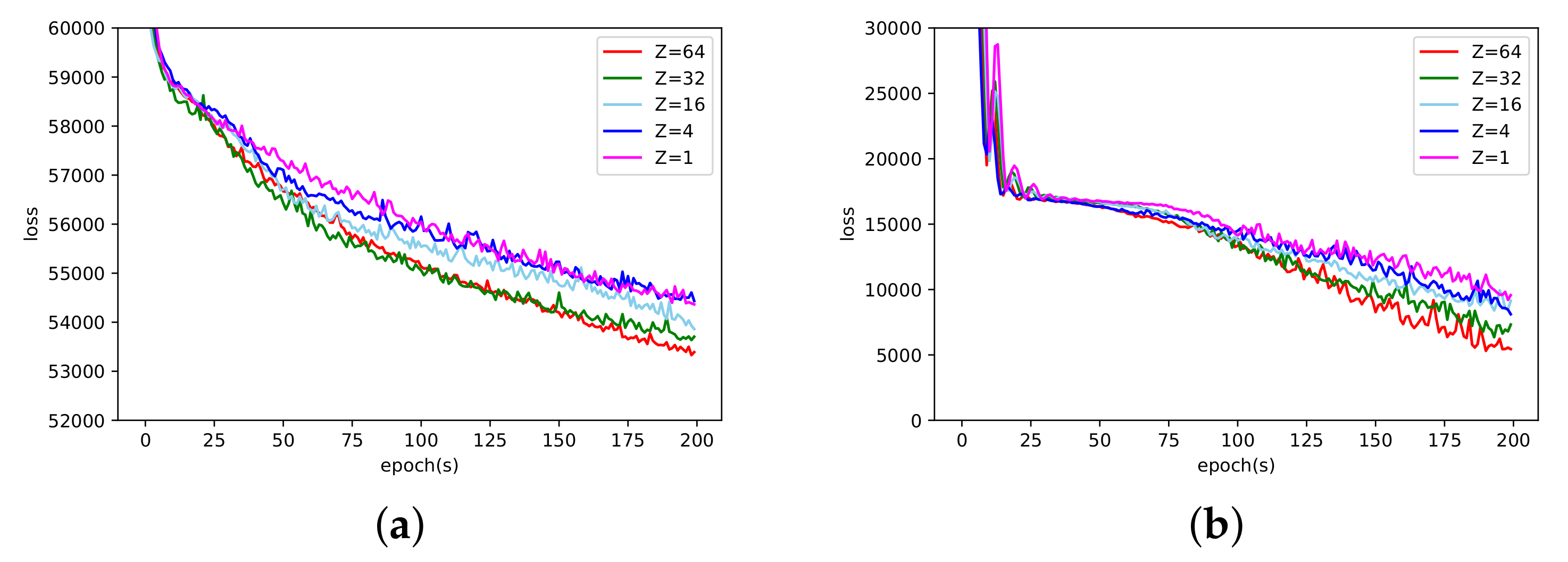
During encoding, a fixed-size memory representation $C\in {\mathbb{R}}^{Z\times D}$ is computed, where Z is a hyperparameter that indicates the number of time-evolving context vectors in the SAEP model, and D is the dimensionality of the cell states. A score vector ${\alpha }_u\in {\mathbb{R}}^Z$ is predicted at each encoding time step u, and the memory representation C in Equation (10) as a linear combination of the encoder states weighted by a score vector ${\alpha }_u$.

$$C_z=\sum _{u=0}^{\left|U\right|}{\alpha }_{uz}{h}_u$$

(10)

$${\alpha }_{uz}=softmax(h_u{W}_{\alpha }\circ l_u)$$

(11)

where $W_{\alpha }$ is a parameter matrix in ${\mathbb{R}}^{Z\times D}$. $l_u$ represents position encoding, which ensures that the context information learned is different. More specifically, because $C_i$ is not necessarily different from $C_{j\ne i}$, the predictions of the context vectors may be symmetric. To enable the model to learn different context information, the position encodings enforce the first few context vectors $C_1,C_2,\cdots$ to focus on the start of the series, and the last few context vectors $\cdots ,C_{Z-1},C_Z$ to focus on the end of the series. To obtain the position encoding $l_u$, it is necessary to compute a constant matrix L. Mathematically, each element of L can be expressed as shown in Equation (12).

$$L_{zu}=(1-\frac{z}{Z})(1-\frac{u}{U})+\frac{z}{Z}\frac{u}{U}$$

(12)

where $z\in \{1,2,\cdots ,Z\}$ denotes the context vector index, and U is the maximum series length across all emotion time series.

In the proposed SAEP model, a standard LSTM network is used as the decoder, which can employ memory representations to reconstruct the original emotion time series. Similar to the encoding phase, a score vector $\beta \in {\mathbb{R}}^Z$ is computed at each decoding step. Then, the time-evolving context vector $\mathbf{a}$ is finally obtained by using Equation (13), which is a linear combination of memory representations weighted by a score vector $\beta$ (Equation (14)).

$$\mathbf{a}=\sum _{z=0}^Z{\beta }_z{C}_z$$

(13)

$$\beta =softmax\left(h^{*}{W}_{\beta }\right)$$

(14)

where $h^{*}$ denotes the current hidden state of the decoder, and $W_{\beta }$ represents the learned parameter matrix. To obtain the current hidden state of the decoder $h_t^{*}$ and the current cell state $c_t^{*}$, with the previous hidden state $h_{t-1}^{*}$, the previous cell state $c_{t-1}^{*}$, and earlier output $x_{t-1}^{*}$ as the input data for the decoder, $h_t^{*}$ is calculated using Equation (15).

$$h_t^{*},c_t^{*}=LSTM(x_{t-1}^{*},h_{t-1}^{*},c_{t-1}^{*})$$

(15)

Algorithm 1 outlines the calculation process for the time-evolving context. First, in the encoding stage, the encoder processes the observed series to obtain the current encoder hidden state $h_u$. Then, a fixed-size memory representation C is obtained, which is a linear combination of the encoder states $h_u$ weighted by the score vector $\alpha$. Finally, in the decoding phase, the memory representation C is weighted by the score vector $\beta$ to obtain the time-evolving context $\mathbf{a}$.

Algorithm 1: Time-evolving context vector calculation

Input: Observed series $X^{{}^{\prime }}$, Time interval series $\Delta T$, Number of time-evolving context vector Z, Dimensionality of the cell states D

Output: Time-evolving context $\mathbf{a}$

1: //Encoding phase

2: Obtain encoder hidden state $h_u$ according to Equation (9).

3: Compute position encoding matrix L by Equation (12);

4: Compute score vector $\alpha$ according to Equation (11).

5: for z from 1 to Z do

6:    Compute fixed-size memory representation $C_z$ by using Equation (10).

7:end for

8: //Decoding phase

9: Obtain decoder hidden state $h^{*}$ by using Equation (15).

10: Calculate score vector $\beta$ according to Equation (14).

11: Compute time-evolving context $\mathbf{a}$ by using Equation (13);

5.4. Surrounding Attention Network

Another important factor is the influence of the social network environment, that is, how neighbor individual emotional states influence each other. In this section, the surrounding attention network, a memory-based attention network similar to the time-evolving attention network, is used to explore the influence of neighboring individual emotional states.

Given a specific user $v_i$, the emotion time series set of their neighbors $\widehat{v}=\{{\widehat{v}}_{\left(1\right)},{\widehat{v}}_{\left(2\right)},$$\cdots ,{\widehat{v}}_{\left(n\right)}\}$ is denoted by $\widehat{X}=\{{\widehat{X}}_{\left(1\right)},{\widehat{X}}_{\left(2\right)},\cdots ,{\widehat{X}}_{\left(n\right)}\}$. Then, the collection of neighbors’ observed series ${\widehat{X}}^{{}^{\prime }}=\{{\widehat{X}}_{\left(1\right)}^{{}^{\prime }},{\widehat{X}}_{\left(2\right)}^{{}^{\prime }},\cdots ,{\widehat{X}}_{\left(n\right)}^{{}^{\prime }}\}$, and the set of time interval series of neighbors $\widehat{\Delta T}=\{{\widehat{\Delta T}}_{\left(1\right)},{\widehat{\Delta T}}_{\left(2\right)},\cdots ,{\widehat{\Delta T}}_{\left(n\right)}\}$ are obtained. For each neighbor ${\widehat{v}}_{\left(n\right)}$, a T-LSTM network encodes their individual emotion time series with the observed series ${\widehat{X}}_{\left(n\right)}^{{}^{\prime }}$ and the time interval series ${\widehat{\Delta T}}_{\left(n\right)}$ as the input data, and obtains the set of encoder’s hidden states $\widehat{h}=\{{\widehat{h}}_{\left(1\right)},{\widehat{h}}_{\left(2\right)},\cdots ,{\widehat{h}}_{\left(n\right)}\}$ by the means of following Equation (16).

$${\widehat{h}}_{u\left(n\right)},{\widehat{c}}_{u\left(n\right)}=T-LSTM({\widehat{x}}_{u\left(n\right)}^{{}^{\prime }},{\widehat{\Delta t}}_{u\left(n\right)},{\widehat{h}}_{u-1\left(n\right)},{\widehat{c}}_{u-1\left(n\right)})$$

(16)

where ${\widehat{h}}_{u\left(n\right)}$ and ${\widehat{c}}_{u\left(n\right)}$ are the hidden state and cell-adjusted state of user $\widehat{v_n}$, respectively. It is important that all parameters in the surrounding attention network are shared by all neighbors.

In the encoding step, the set of neighbors’ memory representations $\widehat{C}=\{{\widehat{C}}_{\left(1\right)},{\widehat{C}}_{\left(2\right)},$$\cdots ,{\widehat{C}}_{\left(n\right)}\}$ is updated, the element ${\widehat{C}}_{\left(n\right)}\in {\mathbb{R}}^{Z\times D}$ is a fixed-size memory representation of the neighbor ${\widehat{v}}_{\left(n\right)}$, where Z is the number of time-evolving context vectors, and D is the size of the cell states. First, a score vector ${\widehat{\alpha }}_{\left(n\right)}$ is obtained by predicting the Z scores at each encoding step. The memory representation ${\widehat{C}}_{\left(n\right)}$ in Equation (17) is then calculated as a weighted sum over a score vector ${\widehat{\alpha }}_{u\left(n\right)}$ (Equation (18)).

$${\widehat{C}}_{z\left(n\right)}=\sum _{u=0}^{\left|U\right|}{\widehat{\alpha }}_{zu\left(n\right)}{\widehat{h}}_{u\left(n\right)}$$

(17)

$${\widehat{\alpha }}_{zu\left(n\right)}=softmax({\widehat{h}}_{u\left(n\right)}{W}_{\widehat{\alpha }}\circ l_u)$$

(18)

where $W_{\widehat{\alpha }}\in {\mathbb{R}}^Z$ denotes a parameter matrix, and $l_u$ is a vector of position encodings that can make the learning attention context different. $l_u$ was calculated using Equation (12). Note that in the surrounding attention network, $W_{\widehat{\alpha }}$ is shared by all neighbors.

The decoding phase of the surrounding attention network is aimed at obtaining the surrounding context vector $\widehat{\mathbf{a}}$. There are slight differences from the calculation of time-evolving context vector in the Section 5.3, the memory representations of the neighbors are used as input, rather than the fixed-size memory representation of a single user. Therefore, the neighbors’ memory representations $\widehat{C}=\{{\widehat{C}}_{\left(1\right)},{\widehat{C}}_{\left(2\right)},\cdots ,{\widehat{C}}_{\left(n\right)}\}$ are concatenated, called surrounding memory representation $\tilde{C}$.

To compute the surrounding context vector $\widehat{\mathbf{a}}$, a score vector $\widehat{\beta }\in {\mathbb{R}}^Z$ is predicted at each decoding step similarly. The surrounding context vector, $\widehat{\mathbf{a}}$ (Equation (19)) is a linear combination of the rows in the surrounding memory representation $\tilde{C}$ weighted by using a Score vector $\widehat{\beta }$ in Equation (20).

$$\widehat{\mathbf{a}}=\sum _{z=0}^Z{\tilde{C}}_z{\widehat{\beta }}_z$$

(19)

$$\widehat{\beta }=softmax\left({\widehat{h}}^{*}{W}_{\widehat{\beta }}\right)$$

(20)

where ${\widehat{h}}^{*}$ is the current hidden state of the decoder, and $W_{\widehat{}\beta }$ is a learned parameter matrix. Similarly, the decoder current hidden state ${\widehat{h}}_t^{*}$ and the current cell state ${\widehat{c}}_t^{*}$ are computed by using Equation (21) and taking the previous hidden state ${\widehat{h}}_{t-1}^{*}$, the previous cell state ${\widehat{c}}_{t-1}^{*}$, and earlier output ${\widehat{x}}_{t-1}^{*}$ as input data:

$${\widehat{h}}_t^{*},{\widehat{c}}_t^{*}=LSTM({\widehat{x}}_{t-1}^{*},{\widehat{h}}_{t-1}^{*},{\widehat{c}}_{t-1}^{*})$$

(21)

Algorithm 2 shows the calculation process for the surrounding context. Initially, for each neighbor ${\widehat{v}}_{\left(n\right)}$, the fixed-size memory representation ${\widehat{C}}_{\left(n\right)}$ is computed. Subsequently, the memory representations of all the neighbors are concatenated to obtain the surrounding memory representation $\tilde{C}$. Then, the surrounding memory representation $\tilde{C}$ is weighted by the score vector $\widehat{\beta }$ to obtain the surrounding context $\widehat{\mathbf{a}}$.

Algorithm 2: Surrounding context vector calculation

Input: The set of observation series $\{{\widehat{X}}_{\left(1\right)}^{{}^{\prime }},{\widehat{X}}_{\left(2\right)}^{{}^{\prime }},\cdots ,{\widehat{X}}_{\left(n\right)}^{{}^{\prime }}\}$, The set of time interval series $\{{\widehat{\Delta T}}_{\left(1\right)},{\widehat{\Delta T}}_{\left(2\right)},\cdots ,{\widehat{\Delta T}}_{\left(n\right)}\}$, Number of time-evolving context vector Z, Dimensionality of the cell states D

Output: Surrounding context vector $\widehat{\mathbf{a}}$

1: //Encoding phase

2: for each neighbor ${\widehat{v}}_{\left(n\right)}$ do

3:     Obtain encoder hidden state ${\widehat{h}}_{u\left(n\right)}$ according to Equation (16);

4:     Compute position encoding matrix L by using Equation (12);

5:     Compute score vector $\widehat{\alpha }$ according to Equation (18);

6:     for z from 1 to Z do

7:         Compute fixed-size memory representation ${\widehat{C}}_{z\left(n\right)}$ by Equation (17);

8:     end for

9: end for

10: Concatenate the neighbors’ memory and obtain surrounding memory representation $\tilde{C}$;

11: //Decoding phase

12: Obtain decoder hidden state ${\widehat{h}}^{*}$ by using Equation (21);

13: Calculate score vector $\widehat{\beta }$ according to Equation (20);

14: Compute surrounding context vector $\widehat{\mathbf{a}}$ by using Equation (19);

The typical attention mechanism used in previous approaches generates a new attention context at each decoding step. In this model, instead of accessing the encoder state at each encoder step, the SAEP model only need to obtain the pre-computed fixed-size memory representation during encoding, which leads to a smaller computational complexity.

5.5. Learning and Prediction

The goal of the present work is to use information from online social networks and time-evolving data to predict future individual emotions. Therefore, the surrounding context vector $\widehat{\mathbf{a}}$ and the time-evolving context vector $\mathbf{a}$ are concatenated. Then, concatenation O is sent to the full connection layer and pass through softmax. The implementation can be expressed by Equations (22) and (23), respectively:

$$O=[\widehat{\mathbf{a}},\mathbf{a}]$$

(22)

$$o^{*}=softmax\left(O{W}_o\right)$$

(23)

where $W_o$ denotes the weight matrix of the fully connected layer. The output $o^{*}$ of the softmax layer is the probability distribution of the final individual emotion category, where the individual emotion category with the highest probability is considered as the individual emotion prediction label. Consequently, the total loss $\mathcal{L}$ is expressed as follows:

$$\mathcal{L}=\sum _{n=1}^N[\sum _{d=1}^D{(o^{d\left(n\right)}-o^{*d\left(n\right)})}^2\times m^{\left(n\right)}]$$

(24)

where N denotes the number of users in the network, and D is the dimensionality of the emotion vector. $o^{d\left(n\right)}$ and $o^{*d\left(n\right)}$ are the predicted and actual emotion vector elements, respectively. $m^{\left(n\right)}$ represents the elements of the masking series.

In the model training phase, SAEP model keeps track of the latest hidden state and all outputs. The last hidden state of the network as the first hidden state of the decoder. A hybrid input strategy is used to feed the data into the feed encoder to speed up the convergence of the model and reduce overfitting. In particular, for some emotion vectors, the actual emotion vector is used as the next input data, if not missing data; otherwise, the decoder’s estimate will be used as the next input data. For the missing emotion vector, the proposed model directly considers the estimated value of the decoder as an alternative value.

Well-trained models can be used to predict individual emotions. Similar to the learning stage, the user’s original individual emotion time series and the neighboring individual emotion time series are processed into the encoder, and obtain the surrounding memory representation and the individual memory representation. In the decoding stage, when an element is not missing, the original individual emotion vector is given; otherwise, the estimated vector is given in order to use as much information as possible from the original emotion time series.

Algorithm 3 summarizes the training and prediction algorithms for SAEP.

Algorithm 3: Training and prediction algorithm for SAEP

Input: Social network $G=(V,E)$, The set of emotion time series $X=\{X_1,X_2,\cdots ,X_n\}$, Number of time-evolving context vector Z, Dimensionality of the cell states D, The number of samples in each batch, The number of epoch

Output:Emotion label

1: Initializing the network structure parameters;

2: for for numbers of training epochs do

3:     for numbers of iteration times do

4:         draw a mini-batch of sequences X and their corresponding neighbors’ context sequence sets $\widehat{X}$;

5:         //forward pass to encoder network

6:         Compute surrounding context vector $\widehat{\mathbf{a}}$;

7:         Compute time-evolving context vector $\mathbf{a}$;

8:         Concatenate surrounding context and time-evolving context by using Equation (22);

9:         Predict emotion by using Equation (23);

10:        Compute the loss function $\mathcal{L}$ according to Equation (24).

11:        //backward pass

12:         Compute gradients;

13:         Update parameters;

14:     end for

15: end for

16: for user $v_i$ in G do

17:     Compute surrounding context vector $\widehat{\mathbf{a}}$;

18:     Compute time-evolving context vector $\mathbf{a}$;

19:     Concatenate surrounding context and time-evolving context by using Equation (22);

20:     Predict emotion by using Equation (23);

21: end for

6. Experiments

6.1. Dataset Description

Experiments on two real-world social network datasets (i.e., Twitter (https://archive.org/details/twitter-iran, accessed on 10 October 2021) and Microblog) were conducted to evaluate the performance of the proposed model. All the datasets and codes are publicly available online (https://github.com/Geoyk96/SAEP, accessed on 10 October 2021). The statistics of the two datasets are shown in

Table 1. Summary of Twitter and Microblog datasets.

Datasets	$\left|\mathit{V}\right|$	$\left|\mathit{E}\right|$	$\mathit{PN}$	$\mathit{RN}$
Twitter	5136	27,142	451,029	705,018
Microblog	5068	12,036	66,480	158,240

( $\left|V\right|$ and $\left|E\right|$ indicate the number of vertices and edges in graph $G=(V,E)$, while $PN$ is the total number of ordinal posts and $RN$ is the total number of reposts).

• Twitter: This dataset sample from 1 November 2015 to 5 March 2016, in which the entire time period has been divided into several time slices in day. For each time slice, the last post from the user within that time (the user’s emotion is influenced by the neighbor and the time-evolving) is saved. In this dataset, the emotion time series size of each user was $125\times 6$. Because users’ post time is irregular, it causes the emotion time series to be missing. The missing data rate of this dataset was $46.70\%$.
• Microblog: The Microblog API is used to randomly download a dataset from Microblog, from 23 January 2018 to 28 April 2018. The same method is used as the Twitter dataset to preprocess and split the Microblog dataset. In this dataset, the emotion time series size of each user was $96\times 6$. The missing data rate of this dataset was $32.64\%$.

6.2. Data Preparation

The basic of this research was to measure emotions. Faced with massive posts, manual tagging is powerless. Instead, tags for automatic post labeling were used, which is a common method in previous studies [47,48]. First, WordNet (http://wordnet.princeton.edu/, accessed on 1 May 2021) and HowNet (http://www.keenage.com/, accessed on 1 May 2021) dictionaries were used to obtain an average of more than 200 synonyms for each basic emotion category and manually verified them.

For the Twitter dataset, a pre-trained RNN [18] was adopted to extract the emotion vectors from the user posts. For each post, the appearances of each emotion synonym category in the texts are computed. If the most frequent emotion corresponds to the emotion vector of the post, then the emotion vector is regarded as the ground truth. Otherwise, it was verified manually. Each post will be reviewed by three different volunteers to eliminate personal bias; then, all the volunteers are required to have a discussion to reach an agreed conclusion. The emotion distribution of this dataset is shown in Figure 7a.

For the Microblog dataset, similar to the Twitter dataset, a pre-trained LSTM [49] was utilized to extract the emotion vectors from users’ posts. The emotion distribution of this dataset is shown in Figure 7b.

6.3. Baseline Methods

• Conditional Random Field (CRF) [47]: It is a graphical model based on conditional random field. The model predicts emotions by combining social correlations with emotional features.
• LSTM [50]: An RNN model with a LSTM cell is trained to predict users’ emotions, which impute the missing data with mean values in emotion time series.
• GRU-D [51]: GRU-D is a novel deep learning model based on GRU. It takes two missing data patterns, masking and time intervals, to extract long-range temporal missing patterns in the time series and capture the informative missing data. GRU-D utilizes long-term temporal dependencies to achieve a better prediction performance.
• Stacked Auto-Encoder (SAE) [52]: SAE is a famous deep learning model, which uses auto encoders as the basic components of deep network. It predicts emotions by learning temporal correlations in the emotion time series.
• Temporal Convolutional Network (TCN) [53]: TCN is a forecasting framework based on convolutional neural network. TCN constructs stacked residual blocks based on dilated causal convolutional networks to capture the temporal dependencies of the emotion time series.

6.4. Hyperparameter Settings

This section discusses the hyperparameter settings. The proposed model uses a 1-layer 32-unit T-LSTM encoder and a 1-layer 32 unit LSTM decoder. The memory size, Z, is 32. The model is optimized using an Adam optimizer with a learning rate of $1\times {10}^{-3}$ in the encoder and $5\times {10}^{-3}$ in the decoder. The batch size was set to 256 and the dropout rate was set to 0.9.

6.5. Evaluation Measures

Multiple criteria are used to evaluate SAEP model, including accuracy ($Acc$) and micro F1 ($Micro\_F1$) [54], which are widely used for evaluating emotion prediction [12,40,55]. Accuracy describes how many of the predicted specific emotion examples were correct. Micro F1 can still make a reasonable evaluation of the classifier in the case of unbalanced samples, which is defined as follows.

$$Precisio{n}_{micro}=\frac{{\sum }_{d=1}^{\left|S\right|}T{P}_d}{{\sum }_{i=1}^{\left|S\right|}T{P}_i+{\sum }_{d=1}^{\left|S\right|}F{P}_d}$$

(25)

$$Recal{l}_{micro}=\frac{{\sum }_{d=1}^{\left|S\right|}T{P}_d}{{\sum }_{d=1}^{\left|S\right|}T{P}_d+{\sum }_{d=1}^{\left|S\right|}F{N}_d}$$

(26)

$$Micro\_F1=2·\frac{Precisio{n}_{micro}·Recal{l}_{micro}}{Precisio{n}_{micro}+Recal{l}_{micro}}$$

(27)

where $Precisio{n}_{micro}$ is micro precision, and $Recal{l}_{micro}$ is micro recall. $T{P}_d$ is the number of emotions correctly predicted as d-th emotion. $F{P}_d$ indicates the number of emotions not labeled as d-th emotion but predicted as d-th emotion. $F{N}_d$ represents the number of emotions incorrectly predicted as d-th emotion. $\left|S\right|$ is the dimension of the emotion vector.

6.6. Performance Comparison

To illustrate the effectiveness of the SAEP model, the performance of the proposed model is compared with that of serval other models, presented in Section 6.3.

Table 2. Performance comparison of emotion prediction of SAEP with five baseline approaches on two datasets.

Dataset	Method		Accuracy
		Anger	Disgust	Fear	Happiness	Sadness	Surprise
Twitter	CRF	79.52	81.25	88.42	72.41	78.28	71.63
	LSTM	80.31	87.75	94.72	74.65	89.17	27.60
	GRU-D	75.92	88.90	93.28	67.52	89.33	74.35
	SAE	72.09	88.58	92.96	55.42	88.67	67.10
	TCN	78.76	81.42	89.09	72.69	85.14	66.00
	SAEP	81.49	83.54	94.49	77.77	89.56	76.44
Microblog	CRF	80.33	81.94	79.36	71.52	82.27	69.38
	LSTM	77.59	87.03	79.68	67.96	82.78	58.83
	GRU-D	76.87	84.87	82.02	67.78	85.00	57.92
	SAE	77.47	87.47	81.76	67.78	84.62	58.19
	TCN	80.91	81.74	80.11	76.32	87.10	64.31
	SAEP	91.31	83.48	91.81	89.23	90.29	87.35

and Figure 8 show the comparative results of different approaches when predicting emotions, and the overall performances of the different approaches on the two datasets are shown in Figure 9. The results for the two datasets show that SAEP model is more competitive.

Table 2 and Figure 9 demonstrate that, although CRF considers some correlation features (the influence between users and neighbors), this method failed to extract the underlying structure in irregular time series data. LSTM can capture the temporal relationships of users’ emotional changes, but LSTM fails to handle irregular time series data, and replacing missing data with average values harms prediction performance. GRU-D designs a recurrent architecture that uses time intervals and masking information to update the missing data. However, it ignores the importance of global temporal background contextual information. SAE is a good approach for predicting emotion, which considers the temporal correlations of emotion changes inherently, but it lacks the modeling of neighbors’ influence. TCN is a kind of convolutional network for time series data, which is with less computation consuming, better ability in capturing individual emotion time-evolving regularities, and higher adaptability for non-linear data. However, it also lacks the modeling of surrounding-influence in social networks. The best comprehensive performance of the SAEP model on two datasets indicates that combining social and temporal contextual information is helpful for predicting users’ future emotions.

As shown in Figure 9, the proposed model significantly outperforms all the baseline methods by achieving the highest micro F1 on the two datasets. The SAEP model improves by 4.21–14.84% and 7.30–13.41% on Twitter and Microblog in terms of micro F1, respectively. The first reason for the better performance of the SAEP model is that the T-LSTM network is employed as the encoder to process irregular time series data, which can better capture the time dependence of emotional states. Second, the proposed model considers the influence of neighbors’ on users’ emotions, which can assist in exploring the changes in emotions between users’ interactions.

6.7. Ablation Analysis

This subsection aims to illustrate the effectiveness of different parts of the proposed model. The SAEP model considers multiple factors that influence users’ emotions in social networks: time-evolving influence and surrounding influence. Moreover, the T-LSTM network is introduced as the encoder of the proposed model to handle irregular emotion time series. Here, this subsection investigated the time-evolving influence, surrounding influence, and T-LSTM encoder to help improve the prediction performance. The contributions of each key component are tested by removing it from the proposed model and comparing their performances. Some variants of the proposed model are listed:

• SAEP: This is the proposed complete model. The parameter settings for this model are described in Section 6.4.
• SAEP-s: This model removes the surrounding attention network.
• SAEP-s-t: This variant removes both surrounding and time-evolving attention networks in the proposed model, meaning it is an RNN with a LSTM cell.
• SAEP-TLSTM: This model employs the standard LSTM as the encoder instead of T-LSTM. The remaining settings for this model are the same as for SAEP model.

The experimental results for the different variants are summarized in

Table 3. Ablation analysis on two datasets.

Dataset	Method		Accuracy
		Anger	Disgust	Fear	Happiness	Sadness	Surprise
Twitter	SAEP-s	80.45	79.6	94.23	75.89	54.96	65.34
	SAEP-s-t	79.84	80.46	94.11	72.2	58.93	71.57
	SAEP-TLSTM	74.42	82.86	93.66	73.67	82.99	64.97
	SAEP	81.49	83.54	94.49	77.77	89.56	76.44
Microblog	SAEP-s	74.85	69.66	88.43	81.58	83.82	65.22
	SAEP-s-t	83.2	68.26	85.62	69.16	85.46	61.15
	SAEP-TLSTM	78.21	67.54	86.94	80.62	87.33	48.84
	SAEP	91.31	83.48	91.81	89.23	90.29	87.35

. Figure 10 further compares the experimental results with the corresponding micro F1. Table 3 illustrates that for most emotion categories, the prediction performance will be lower when each of the three key components is removed.

Previous studies have revealed that social information plays a crucial role in image-based emotion prediction tasks [47,48]. The experimental results further verify that the surrounding influence can also help improve the performance of text-based tasks, especially on the Microblog dataset. Table 3 indicates that the performance of SAEP model is better than that of SAEP-s on two datasets, which indicates that the surrounding attention network can effectively model the surrounding influence. SAEP-s outperforms SAEP-s-t model in terms of micro F1 on the two datasets. This is because the time-evolving attention network can capture the complex patterns of emotions that evolve over time.

In addition, the performance of SAEP-TLSTM is not as good as that of the proposed complete model SAEP, which illustrates the decrease in the micro F1 when using the standard LSTM network as the encoder of the SAEP model. Evidently, T-LSTM as the encoder can effectively process irregular time series data, and in this way, the model performance is improved significantly. It is easily concluded that by using T-LSTM network to process irregular time series data and fusing time-evolving and surrounding influences, the SAEP model achieves the best prediction performance. Figure 10 suggests that the overall performances of the proposed complete model (SAEP) are better than that of the variants.

6.8. Parameter Analysis

To achieve the optimal prediction performance of the SAEP model, this subsection explored how different hyperparameters affect the performance of the proposed model. These include cell size D and memory size Z, which are hyperparameters related to model tuning. Extensive experiments were conducted by adjusting only the relevant hyperparameters to achieve the best performance while keeping the other hyperparameters unchanged.

6.8.1. Effect of Cell Size for Prediction Accuracy

The impact of D is explored, which is an important hyperparameter on the prediction performance of SAEP. Figure 11 shows the effect of D on model prediction performance on two datasets. In Figure 11, the prediction performance changes as the hyperparameter varies. It should be noted that in Figure 11, if the cell size D is too small or too large, the prediction micro F1 of SAEP tends to worsen. This indicates that selecting a proper cell size D is crucial for model performance.

6.8.2. Effect of Memory Size for Predict Accuracy

This subsection aims to evaluate the influence of memory size Z. This study examines the trade-off between computational time and representational power. A large Z allows the model to calculate complex source representations, whereas $Z=1$ limits the source representation to a single vector. The influence of Z on the prediction performance is shown in Figure 12. It can be seen that within a certain range, the performance of the proposed model improves.

6.8.3. Effect of Memory Size for Learning Procedure

Here, an experiment was conducted to observe the effect of varying values of the hyperparameter Z on the learning process. Figure 13a,b show the learning curves. It can be seen that the proposed model has a faster convergence while memory size Z increases on both datasets. Specifically, notice that $Z=1$ fails to fit the data distribution. When the Z value increases, the SAEP model representation ability is enhanced, which significantly speeds up the inference process.

6.9. Visualization

Finally, the emotion prediction results of different methods are visualized. Figure 14 shows the comparison of the seven methods on Microblog dataset. Figure 14a depicts the true emotions of users in Microblog social network in the future. Figure 14b represents the visualization result obtained by the proposed model. Figure 14c–g shows the results of the other five approaches. In terms of the micro F1 of emotion prediction, SAEP, CRF, LSTM, GRU-D, SAE, TCN reached 63.33%, 52.75%, 49.92%, 50.74%, 54.50%, and 56.03%, respectively.

Figure 14b intuitively illustrates that the emotions predicted by the SAEP model are more in line with the real situation. Differences occur in the prediction performance between these baseline methods and the proposed model, and these differences can be explained from two aspects. First, SAEP not only considers the changing trend of the user’s emotions, but also considers the influence of the emotions of the user’s neighbors on the user. Second, the proposed model introduces a T-LSTM network to handle irregular emotion time series, which can effectively extract the underlying structure in the irregular emotion time series. In addition, Figure 14a indicates that neighboring users have a greater probability of similar emotions. This can be explained by the emotional influence of the neighbors.

7. Conclusions

The widespread use of social media has facilitated people’s communication as well as the emotion propagation in social networks greatly, and is therefore bringing the enormous impacts on social psychological cognition and group behaviors than ever before. This issue of emotion prediction on social media has become a new concerning hot point in social media analytics.

This paper aims to predict individuals’ future emotions and a surrounding-aware individual emotion prediction model-based deep encoder–decoder architecture is proposed for individual future emotion prediction by considering the influence of time-evolving and individual’s neighbors. Based on individual emotion time series, the time-evolving attention network extracts the memory representation of an individual to obtain the time-evolving context to better capture the individual emotional change rule and emotional preference. The surrounding attention network obtains the surrounding context from the set of neighbors’ emotion time series to better learn the influence of neighbors’ emotions.

Experiments on two datasets (from two social networks) demonstrate that the SAEP model achieves good results and outperforms several baseline methods for emotion prediction. In addition, this paper validated the effectiveness of the proposed time-evolving influence and surrounding influence by means of ablation experiments, which proves the importance of surrounding influence and time-evolving influence in predicting individuals’ future emotions. Futhermore, research findings in ablation experiments indicated that T-LSTM network as the basic component of SAEP model to encode an irregular time series have significant impacts on the model performance. Moreover, to explore the influence of different hyperparameters on the model performance and minimize system load, parameter analysis experiments are conducted. The emotion prediction results of different methods on Microblog are visualized to intuitively understand the effectiveness of the SAEP model.

In the future, more effective patterns in social networks to predict individual emotions will be explored, such as changes in user relationships and user interactions. Simultaneously, a new neural network technology will be used to enhance performance. Furthermore, whether the method can be applied in other heterogeneous networks needs to be further explored.

References

1. Shahriar, S.; Kim, Y. Audio-Visual Emotion Forecasting: Characterizing and Predicting Future Emotion Using Deep Learning. In Proceedings of the 2019 14th IEEE International Conference on Automatic Face Gesture Recognition, Lille, France, 14–18 May 2019; pp. 1–7. [Google Scholar] [CrossRef]
2. Yamane, H.; Mori, Y.; Harada, T. Humor meets morality: Joke generation based on moral judgement. Inf. Process. Manag. 2021, 58, 102520. [Google Scholar] [CrossRef]
3. Ge, Y.; Qiu, J.; Liu, Z.; Gu, W.; Xu, L. Beyond negative and positive: Exploring the effects of emotions in social media during the stock market crash. Inf. Process. Manag. 2020, 57, 102218. [Google Scholar] [CrossRef]
4. Du, Y.; Zhou, Q.; Luo, J.; Li, X.; Hu, J. Detection of key figures in social networks by combining harmonic modularity with community structure-regulated network embedding. Inf. Sci. 2021, 570, 722–743. [Google Scholar] [CrossRef]
5. Gong, C.; Du, Y.; Li, X.; Chen, X.; Li, X.; Wang, Y.; Zhou, Q. Structural hole-based approach to control public opinion in a social network. Eng. Appl. Artif. Intell. 2020, 93, 103690. [Google Scholar] [CrossRef]
6. Li, Y.; Wang, S.; Pan, Q.; Peng, H.; Yang, T.; Cambria, E. Learning binary codes with neural collaborative filtering for efficient recommendation systems. Knowl.-Based Syst. 2019, 172, 64–75. [Google Scholar] [CrossRef]
7. Lomanowska, A.M.; Guitton, M.J. Online intimacy and well-being in the digital age. Internet Interv. 2016, 4, 138–144. [Google Scholar] [CrossRef] [Green Version]
8. Hill, A.L.; Rand, D.G.; Nowak, M.A.; Christakis, N.A. Emotions as infectious diseases in a large social network: The SISa model. Proc. R. Soc. B 2010, 277, 3827–3835. [Google Scholar] [CrossRef]
9. Bond, R.M.; Fariss, C.J.; Jones, J.J.; Kramer, A.D.I.; Marlow, C.; Settle, J.E.; Fowler, J.H. A 61-million-person experiment in social influence and political mobilization. Nature 2012, 489, 295–298. [Google Scholar] [CrossRef] [Green Version]
10. Neil, D.; Pfeiffer, M.; Liu, S.C. Phased LSTM: Accelerating Recurrent Network Training for Long or Event-Based Sequences. In Proceedings of the 30th International Conference on Neural Information Processing Systems, Barcelona, Spain, 5–10 December 2016; pp. 3889–3897. [Google Scholar]
11. Ekman, P. An argument for basic emotions. Cogn. Emot. 1992, 6, 169–200. [Google Scholar] [CrossRef]
12. Yang, Y.; Jia, J.; Wu, B.; Tang, J. Social Role-Aware Emotion Contagion in Image Social Networks. In Proceedings of the 30th AAAI Conference on Artificial Intelligence, Phoenix, AZ, USA, 12–17 February 2016; pp. 65–71. [Google Scholar]
13. Keshavarz, H.; Abadeh, M.S. ALGA: Adaptive lexicon learning using genetic algorithm for sentiment analysis of microblogs. Knowl.-Based Syst. 2017, 122, 1–16. [Google Scholar] [CrossRef] [Green Version]
14. Chekima, K.; Alfred, R. Non-English Sentiment Dictionary Construction. Adv. Sci. Lett. 2018, 24, 1416–1420. [Google Scholar] [CrossRef]
15. Song, J.; Kim, K.; Lee, B.; Kim, S.; Youn, H. A novel classification approach based on Naive Bayes for Twitter sentiment analysis. KSII Trans. Internet Inf. Syst. 2017, 11, 2996–3011. [Google Scholar] [CrossRef]
16. Liu, Y.; Bi, J.W.; Fan, Z.P. A method for multi-class sentiment classification based on an improved one-vs-one (OVO) strategy and the support vector machine (SVM) algorithm. Inf. Sci. 2017, 394–395, 38–52. [Google Scholar] [CrossRef] [Green Version]
17. Xie, X.; Ge, S.; Hu, F.; Xie, M.; Jiang, N. An Improved Algorithm for Sentiment Analysis Based on Maximum Entropy. Soft Comput. 2019, 23, 599–611. [Google Scholar] [CrossRef]
18. Colnerič, N.; Demšar, J. Emotion Recognition on Twitter: Comparative Study and Training a Unison Model. IEEE Trans. Affect. Comput. 2020, 11, 433–446. [Google Scholar] [CrossRef]
19. Wang, Y.; Huang, M.; Zhao, L.; Zhu, X. Attention-based LSTM for Aspect-level Sentiment Classification. In Proceedings of the 2016 Conference on Empirical Methods in Natural Language Processing, Austin, TX, USA, 1–5 November 2016; pp. 606–615. [Google Scholar]
20. Wang, R.; Li, Z.; Cao, J.; Chen, T.; Wang, L. Convolutional Recurrent Neural Networks for Text Classification. In Proceedings of the 2019 International Joint Conference on Neural Networks, Budapest, Hungary, 14–19 July 2019; pp. 1–6. [Google Scholar] [CrossRef]
21. Cambria, E. Affective Computing and Sentiment Analysis. IEEE Intell. Syst. 2016, 31, 102–107. [Google Scholar] [CrossRef]
22. Borg, A.; Boldt, M. Using VADER sentiment and SVM for predicting customer response sentiment. Expert Syst. Appl. 2020, 162, 113746. [Google Scholar] [CrossRef]
23. Adikari, A.; Gamage, G.; de Silva, D.; Mills, N.; Wong, S.M.J.; Alahakoon, D. A self structuring artificial intelligence framework for deep emotions modeling and analysis on the social web. Future Gener. Comput. Syst. 2021, 116, 302–315. [Google Scholar] [CrossRef]
24. Zhang, X.; Li, W.; Ying, H.; Li, F.; Tang, S.; Lu, S. Emotion Detection in Online Social Networks: A Multilabel Learning Approach. IEEE Internet Things J. 2020, 7, 8133–8143. [Google Scholar] [CrossRef]
25. Wang, Y.; Han, L. Adaptive time series prediction and recommendation. Inf. Process. Manag. 2021, 58, 102494. [Google Scholar] [CrossRef]
26. Luo, Y.; Yao, C.; Mo, Y.; Xie, B.; Yang, G.; Gui, H. A creative approach to understanding the hidden information within the business data using Deep Learning. Inf. Process. Manag. 2021, 58, 102615. [Google Scholar] [CrossRef]
27. Majumder, N.; Poria, S.; Hazarika, D.; Mihalcea, R.; Cambria, E. DialogueRNN: An attentive rnn for emotion detection in conversations. In Proceedings of the 33rd AAAI Conference on Artificial Intelligence, Honolulu, HI, USA, 27 January–1 February 2019; pp. 6818–6825. [Google Scholar] [CrossRef] [Green Version]
28. Ma, J.; Tang, H.; Zheng, W.L.; Lu, B.L. Emotion Recognition Using Multimodal Residual LSTM Network. In Proceedings of the 27th ACM International Conference on Multimedia, Nice, France, 21–25 October 2019; pp. 176–183. [Google Scholar] [CrossRef]
29. Cho, K.; van Merriënboer, B.; Gulcehre, C.; Bahdanau, D.; Bougares, F.; Schwenk, H.; Bengio, Y. Learning Phrase Representations using RNN Encoder–Decoder for Statistical Machine Translation. In Proceedings of the 2014 Conference on Empirical Methods in Natural Language Processing, Doha, Qatar, 25–29 October 2014; pp. 1724–1734. [Google Scholar] [CrossRef]
30. Zhang, R.; Wang, Z.; Huang, Z.; Li, L.; Zheng, M. Predicting Emotion Reactions for Human—Computer Conversation: A Variational Approach. IEEE Trans.-Hum.-Mach. Syst. 2021, 51, 279–287. [Google Scholar] [CrossRef]
31. Lubis, N.; Sakti, S.; Yoshino, K.; Nakamura, S. Positive Emotion Elicitation in Chat-Based Dialogue Systems. IEEE/ACM Trans. Audio Speech Lang. Process. 2019, 27, 866–877. [Google Scholar] [CrossRef]
32. Liu, M.; Bao, X.; Liu, J.; Zhao, P.; Shen, Y. Generating emotional response by conditional variational auto-encoder in open-domain dialogue system. Neurocomputing 2021, 460, 106–116. [Google Scholar] [CrossRef]
33. Li, D.; Li, Y.; Wang, S. Interactive double states emotion cell model for textual dialogue emotion prediction. Knowl.-Based Syst. 2020, 189, 105084. [Google Scholar] [CrossRef]
34. Tang, H.; Ji, D.; Zhou, Q. Joint multi-level attentional model for emotion detection and emotion-cause pair extraction. Neurocomputing 2020, 409, 329–340. [Google Scholar] [CrossRef]
35. Devlin, J.; Chang, M.W.; Lee, K.; Toutanova, K. BERT: Pre-training of Deep Bidirectional Transformers for Language Understanding. In Proceedings of the 2019 Conference of the North American Chapter of the Association for Computational Linguistics: Human Language Technologies, Minneapolis, MN, USA, 2–7 June 2019; pp. 4171–4186. [Google Scholar]
36. Sun, X.; Li, J.; Wei, X.; Li, C.; Tao, J. Emotional editing constraint conversation content generation based on reinforcement learning. Inf. Fusion 2020, 56, 70–80. [Google Scholar] [CrossRef]
37. Huang, X.; Ren, M.; Han, Q.; Shi, X.; Nie, J.; Nie, W.; Liu, A.A. Emotion Detection for Conversations Based on Reinforcement Learning Framework. IEEE Multimed. 2021, 28, 76–85. [Google Scholar] [CrossRef]
38. Ma, H.; Wang, J.; Qian, L.; Lin, H. HAN-ReGRU: Hierarchical attention network with residual gated recurrent unit for emotion recognition in conversation. Neural Comput. Appl. 2021, 33, 2685–2703. [Google Scholar] [CrossRef]
39. Li, W.; Shao, W.; Ji, S.; Cambria, E. BiERU: Bidirectional emotional recurrent unit for conversational sentiment analysis. Neurocomputing 2022, 467, 73–82. [Google Scholar] [CrossRef]
40. Tang, J.; Zhang, Y.; Sun, J.; Rao, J.; Yu, W.; Chen, Y.; Fong, A. Quantitative Study of Individual Emotional States in Social Networks. IEEE Trans. Affect. Comput. 2012, 3, 132–144. [Google Scholar] [CrossRef]
41. Gökdağ, C. How does interpersonal emotion regulation explain psychological distress? The roles of attachment style and social support. Personal. Individ. Differ. 2021, 176, 110763. [Google Scholar] [CrossRef]
42. Hochreiter, S.; Schmidhuber, J. Long Short-Term Memory. Neural Comput. 1997, 9, 1735–1780. [Google Scholar] [CrossRef]
43. Weerakody, P.B.; Wong, K.W.; Wang, G.; Ela, W. A review of irregular time series data handling with gated recurrent neural networks. Neurocomputing 2021, 441, 161–178. [Google Scholar] [CrossRef]
44. Baytas, I.M.; Xiao, C.; Zhang, X.; Wang, F.; Jain, A.K.; Zhou, J. Patient Subtyping via Time-Aware LSTM Networks. In Proceedings of the 23th ACM SIGKDD International Conference on Knowledge Discovery and Data Mining, Halifax, NS, Canada, 13–17 August 2017; pp. 65–74. [Google Scholar] [CrossRef]
45. Ji, Y.; Zhang, H.; Zhang, Z.; Liu, M. CNN-based encoder–decoder networks for salient object detection: A comprehensive review and recent advances. Inf. Sci. 2021, 546, 835–857. [Google Scholar] [CrossRef]
46. Britz, D.; Guan, M.; Luong, M.T. Efficient Attention using a Fixed-Size Memory Representation. In Proceedings of the 2017 Conference on Empirical Methods in Natural Language Processing, Copenhagen, Denmark, 9–11 September 2017; pp. 392–400. [Google Scholar] [CrossRef] [Green Version]
47. Wang, X.; Jia, J.; Tang, J.; Wu, B.; Cai, L.; Xie, L. Modeling Emotion Influence in Image Social Networks. IEEE Trans. Affect. Comput. 2015, 6, 286–297. [Google Scholar] [CrossRef] [Green Version]
48. Yang, Y.; Jia, J.; Zhang, S.; Wu, B.; Chen, Q.; Li, J.; Xing, C.; Tang, J. How Do Your Friends on Social Media Disclose Your Emotions? In Proceedings of the 28th AAAI Conference on Artificial Intelligence, Québec City, QC, Canada, 27–31 July 2014; pp. 306–312. [Google Scholar]
49. Yuan, Z.; Purver, M. Predicting Emotion Labels for Chinese Microblog Texts. In Proceedings of the 1st International Workshop on Sentiment Discovery from Affective Data, Bristol, UK, 28 September 2012; Volume 917, pp. 40–47. [Google Scholar]
50. Yang, B.; Sun, S.; Li, J.; Lin, X.; Tian, Y. Traffic flow prediction using LSTM with feature enhancement. Neurocomputing 2019, 332, 320–327. [Google Scholar] [CrossRef]
51. Che, Z.; Purushotham, S.; Cho, K.; Sontag, D.; Liu, Y. Recurrent Neural Networks for Multivariate Time Series with Missing Values. Sci. Rep. 2018, 8, 6085. [Google Scholar] [CrossRef] [Green Version]
52. Lv, Y.; Duan, Y.; Kang, W.; Li, Z.; Wang, F.Y. Traffic Flow Prediction With Big Data: A Deep Learning Approach. IEEE Trans. Intell. Transp. Syst. 2015, 16, 865–873. [Google Scholar] [CrossRef]
53. Chen, Y.; Kang, Y.; Chen, Y.; Wang, Z. Probabilistic forecasting with temporal convolutional neural network. Neurocomputing 2020, 399, 491–501. [Google Scholar] [CrossRef] [Green Version]
54. Yang, T.; Li, F.; Ji, D.; Liang, X.; Xie, T.; Tian, S.; Li, B.; Liang, P. Fine-grained depression analysis based on Chinese micro-blog reviews. Inf. Process. Manag. 2021, 58, 102681. [Google Scholar] [CrossRef]
55. Li, Y.; Huang, X.; Zhao, G. Micro-expression action unit detection with spatial and channel attention. Neurocomputing 2021, 436, 221–231. [Google Scholar] [CrossRef]
Figure 1. Illustration of the surrounding-aware individual emotion prediction problem.
Applsci 11 11111 g001
Figure 2. Example of the emotion time series X, observed series X , masking series M, time interval series Δ T .
Applsci 11 11111 g002
Figure 3. Individual emotional state transition matrix.
Applsci 11 11111 g003
Figure 4. Correlation between neighbors’ emotions and user’s future emotion.
Applsci 11 11111 g004
Figure 5. Basic process of SAEP model.
Applsci 11 11111 g005
Figure 6. Illustration of the time-aware long-short term memory (T-LSTM) unit.
Applsci 11 11111 g006
Figure 7. Percent of per emotion category on two datasets. (a) Twitter; (b) Microblog.
Applsci 11 11111 g007
Figure 8. Comparison of the accuracy of different emotion categories with different methods (a) Anger (b) Disgust (c) Fear (d) Happiness (e) Sadness (f) Surprise.
Applsci 11 11111 g008
Figure 9. Emotion prediction results “micro F1” on two datasets. (a) Twitter; (b) Microblog.
Applsci 11 11111 g009
Figure 10. Ablation analysis results “micro F1” on two datasets. (a) Twitter; (b) Microblog.
Applsci 11 11111 g010
Figure 11. Model parameter analysis (cell size D).
Applsci 11 11111 g011
Figure 12. Model parameter analysis (Memory size Z).
Applsci 11 11111 g012
Figure 13. Comparison concerning varying memory size Z for the training loss curve on two datasets. (a) Twitter; (b) Microblog.
Applsci 11 11111 g013
Figure 14. Visualization of emotion prediction with different methods on Microblog (a) Original (b) SAEP (c) CRF (d) LSTM (e) GRU-D (f) SAE (g) TCN.
Applsci 11 11111 g014