Attention to Fires: Multi-Channel Deep Learning Models for Wildfire Severity Prediction

Abstract

Wildfires are one of the natural hazards that the European Union is actively monitoring through the Copernicus EMS Earth observation program which continuously releases public information related to such catastrophic events. Such occurrences are the cause of both short- and long-term damages. Thus, to limit their impact and plan the restoration process, a rapid intervention by authorities is needed, which can be enhanced by the use of satellite imagery and automatic burned area delineation methodologies, accelerating the response and the decision-making processes. In this context, we analyze the burned area severity estimation problem by exploiting a state-of-the-art deep learning framework. Experimental results compare different model architectures and loss functions on a very large real-world Sentinel2 satellite dataset. Furthermore, a novel multi-channel attention-based analysis is presented to uncover the prediction behaviour and provide model interpretability. A perturbation mechanism is applied to an attention-based DS-UNet to evaluate the contribution of different domain-driven groups of channels to the severity estimation problem.

1. Introduction

In the last decade, the attention to environmental problems significantly increased to safeguard natural resources [1,2], preserve flora and fauna and the different ecosystems, and prevent catastrophic events and natural disasters. Among such natural disasters, forest fires demonstrated an increasing trend in recent years [3,4], causing large losses and damages to ecosystems and municipalities. In this paper, we focus our attention on the increasing problem of forest fires, which are causes of both short- and long-term damages: economical loss, environmental damages  [5,6], and high risk for living beings, but also higher risk of soil erosion  [7] and high recovery time due to reforestation. As a consequence of such disasters, the importance and the ability to monitor forests and affected areas are becoming crucial in decision-making processes led by authorities and governments  [8]. As such, the need for proper tools and data is indeed relevant to the field: open data, aerial data acquisitions through aircraft, drones, and satellite imagery represent important ways to timely collect data and evaluate critical information, especially in times of natural disasters.

Thanks to the availability of high-resolution images from Sentinel-1 and Sentinel-2 missions, the adoption of satellite acquisitions by the scientific community is growing. As an example, the work in  [9] analyzed the problem of tree mortality leveraging on satellite imagery and forest surveys, whereas the work in [10] proposed the integration of multispectral satellite data for rapid assessment of forest damage caused by extreme events, such as storms. Therefore, the implementation of machine learning and deep learning models combined with large scale satellite imagery enables the research community and public authorities to analyze areas at a continental scale in a short amount of time, providing useful insights to decision-makers. More specifically, convolutional neural networks (CNNs) for satellite image analyses proved to be extremely effective in detecting forest wildfires and burnt area detection [11,12,13].

In this paper, we focus on the adoption of state-of-the-art deep learning segmentation models applied to satellite acquisition to automatically detect areas damaged by previous forest wildfires and provide a discrete severity level estimation within fixed ranges. In particular, we investigate multi-channel explainability strategies driven by the introduction of an attention mechanism in the segmentation models. To the best of our knowledge, no previous works introduced an attention-driven mechanism to support the interpretability of multi-channel deep learning models in the field of automatic burned area detection, providing benefits in decision support systems and supporting local authorities’ operations during the environmental monitoring processes.

The novel contributions of the current work can be summarized as follows:

• Extensive experimental comparison of a wide range of model architectures and loss functions for deep learning wildfire severity prediction models on real-world satellite data.
• Application of state-of-the-art deep-learning models to a very large dataset (24 GB) for wildfire severity prediction.
• Extension of a state-of-the-art Double-Step deep learning Framework (DSF) by introducing an attention mechanism to the UNet segmentation model.
• Analysis of multi-channel model interpretability by exploiting both the newly introduced attention-based mechanism and domain knowledge.

The paper is structured as follows. Section 2 introduces the related works. Section 3 describes the proposed state-of-the-art Double-Step deep learning Framework (DSF) and all its components. Section 4 describes the dataset, the experimental design, and discusses the results. Finally, Section 5 presents conclusions and future developments.

2. Related Work

In this section, we first review previous works on different strategies for wildfire prediction. Then, moving to the CNN solutions, we analyze the state-of-the-art architectures addressing semantic segmentation problems, and we focus on applying these techniques to our task, highlighting the differences with our proposed solution. Finally, in Section 2.1, we provide an overview of the available explainability techniques suitable for the computer vision domain.

Burnt area delineation is a well-known problem in remote sensing literature. Many approaches address this task by exploiting different satellite indexes techniques [14,15], eventually assessing a severity level estimation [16,17]. Satellites collect information across multiple bandwidths which are sensitive to different land features. Therefore, combinations of specific acquisition channels can be used to detect the presence of water bodies [18], vegetation [19], burnt areas [20], snow, and, in principle, any kind of terrain [21,22,23,24] with the application of thresholding strategies [25] such as the Otsu’s method [26,27]. These combinations of acquisition channels are known in the literature as indexes.

Normalized Burn Ratio (NBR) [28,29] and Burned Area Index for Sentinel-2 (BAIS2) [20] are some of the aforementioned indexes specifically designed for burned area detection. Considering the 12 bandwidths available from Sentinel-2 L2A products, NBR is the normalized difference between the Near-Infrared (NIR) and the short wavelength infrared (SWIR) channels (8 and 12, respectively). BAIS2 instead combines vegetation properties obtained from a band ratio in the red-edge spectral domain (bands 6 and 7) and a band ratio involving bands 8A and 12, recognized to be efficient in determining burnt regions. Further indexes can be obtained by comparing pre-fire and post-fire acquisitions, as for delta Normalized Burn Ratio (dNBR) [16], computed as $\mathrm{dNBR}={\mathrm{NBR}}_{PRE}-{\mathrm{NBR}}_{POST}$. Then, the dNBR can be quantized to generate a severity scale. This approach is computationally fast and is generally considered very accurate. Therefore, it is still largely adopted by the scientific community [17,30]. The European Forest Fire Information Service (EFFIS) of Copernicus program itself provides, in fact, an adjusted threshold for dNBR to identify four different severity levels [31].

Severity prediction based on manual or automatic thresholding of these indexes is addressed with a wide range of techniques [25,32,33]. However, dNBR also requires acquisitions taken before the wildfire event, which might be difficult to obtain. Depending on season and weather conditions, atmosphere, foliage, and ground morphology can sensibly change. Moreover, cloud coverage can affect the visibility of the areas of interest (AoI), making the comparison between pre- and post-fire images difficult overall. Summing up, generated maps such as the ones provided by Copernicus EMS requires several days to be completed and an eventual manual intervention, as the homogeneity between the two events is not guaranteed. Some mapping operations are performed based on in situ information, such as the Composite Burned Index (CBI) [34], but these are time-consuming and require a large amount of extra data such as the evaluations of the soil and vegetation conditions for the entire AoI.

These limitations offer the opportunity to investigate many different approaches, eventually involving machine learning and deep learning-based techniques, such as in [35,36]. Deep learning strategies have been largely adopted in the past to address many kinds of predictions concerning wildfire events. Some techniques, such as those in [37,38], can, for instance, be used to monitor the evolution of wildfires during the event to support domain experts. Moving to the damaged region analysis, our proposed solutions solve the aforementioned issues by only considering post-fire images and applying a supervised prediction approach on pre-labeled severity maps. Specifically, we treat the wildfire delineation and the severity prediction as image segmentation tasks. Such a problem is highly present in the medical imaging field, in which the literature proposes a series of neural network architectures [39,40,41]. Many works in remote sensing make large use of networks such as U-Net [42], which is particularly suitable for analysis on small datasets. Li et al., in [43], use this architecture on Sentinel-2 images to map salt marsh along the coasts, while others apply similar techniques to the segmentation of forests [44] or cloud coverage [45]. Concerning wildfire detection, different works as those in [11,46] address the task via CNN models, but they lack to answer the damage level assessment question.

Among many other semantic segmentation architectures which have been proposed in literature [47,48,49], the works in [50,51] demonstrated the U-Net architecture to be a valuable choice for the wildfire damage severity estimation problem. The state-of-the-art solution proposes a Double-Step U-Net architecture, addressing the wildfire delineation and the severity prediction tasks separately. This double-step configuration relies on the Binary Cross-Entropy (BCE) loss function on the first stage and on the Mean Squared Error (MSE) loss on the second stage to estimate the final severity level. It is a straightforward fact that a proper choice of model and loss functions can significantly improve the performance of the models, as shown in [52,53]. For this reason, the goal of this work is to validate and extend the results in [54], testing the proposed models to a widely extended set of images, and introducing a multi-channel interpretability analysis by exploiting both domain knowledge and a newly added attention-based mechanism. Analyzing the contribution of different channels to the prediction provides insights into the contributions of each channel to the deep learning model reasoning, a task which is typically addressed in Explainable Artificial Intelligence.

2.1. Explainable Artificial Intelligence

Despite the high accuracy of deep neural networks such as CNN on image classification and segmentation tasks, their complex architecture hides their decision-making process. The lack of comprehensibility increases the need to explain and understand their decisions. This has led to the growth of a new research area called eXplainable Artificial Intelligence (XAI).

The different literature explainability techniques can be classified according to various criteria [55]. The first possible classification is by the scope of the explanation: (i) local explanation and (ii) global explanation. The former aims to explain single predictions of the model, while the latter explains the model at a global level. Then, the explanations can be classified as intrinsic if they are obtained by approximating them with an interpretable white-box model, and in post hoc, if they analyze the model after training. A further classification is (i) model-agnostic and (ii) model-specific. Model-agnostic methods can be applied to any model, while model-specific techniques are limited to specific model architectures. Finally, explanation methodologies can be classified by how they are produced, and the most common are: (i) gradient-based and (ii) perturbation-based explanations.

Gradient-based explanations [56,57] are powerful methods that measure the spatial importance of a particular class in images by exploiting the gradients of the outputs over inputs and class activation mapping (CAM) [58] to show relevant portions of the input images. Other similar techniques instead exploit saliency maps [59,60,61]. In contrast, perturbation-based explanations evaluate how the outputs are affected by inputs’ changes. For instance, the work in [62] uses a model-agnostic perturbation-based technique that produces local explanations by training a simpler interpretable model that approximates the prediction locally. Instead, the work in [63] produces local explanations of deep convolutional neural networks by a process of perturbation over interpretable features extracted from the hypercolumns. The authors of [64] propose a model-agnostic explainability technique based on a game-theoretic approach that iteratively removes combinations of inputs features to measure the features’ importance.

Both gradient- and perturbation-based methods usually exploit heatmaps or similar techniques to visualize the relevant pixels on the RGB channels to produce explanations. However, most of these techniques were originally intended to explain classification models. A first attempt to perform explainability on segmentation models was proposed in [65]. It implements various gradient-based visualization methods helping to understand and visualize different layers of neural networks to explain its predictions. In our case, landing data for wildfire severity prediction is composed of complex multi-channel inputs with different bands besides RGB, making human understandability difficult. Moreover, the aggregations of different channels have different and important domain-driven meanings.

This increases the need to analyze inputs based on the domain semantics. Therefore, an explanation that visualizes only RGB channels would not be effective, especially for domain experts.

Differently from previous works, in this paper, we combine a model-aware attention-driven post hoc perturbation technique with landing wildfire domain knowledge to globally explain deep convolutional segmentation models by understanding the most relevant inputs macro-bands. To the best of our knowledge, this is the first attempt to interpreting and explaining the segmentation of deep neural networks for wildfire severity prediction.

3. Double-Step Deep-Learning Framework (DSF)

In this section, we recall the Double-Step deep learning Framework (DSF) in [54] as a state-of-the-art approach addressing the wildfire severity prediction problem. The DSF splits the task between a first wildfire binary detection and a consequent severity prediction. Such a framework allows complete customization of both training loss functions and backbone neural networks. The main building blocks of the DSF, separated into the two tasks, are depicted in Figure 1 and are described in terms of functionalities in the following section. Such backbones can be customized to obtain different configurations.

3.1. Wildfire Detection Task (First Step)

Binary-class backbone. This building block takes the satellite images and assigns to each pixel a binary label (i.e., burnt or unburnt) regardless of the severity values of the wildfire. Its output is a probability map with values in the range [0, 1]. The actual components taken into account are summarized in Section 3.3.

Binary loss. The first backbone training is performed using an intermediate loss function, constructed to compare the probability output with the ground-truth binary mask. At this stage, among all the possible alternatives in the literature, we focus on different standard and custom prediction loss functions depending on the features we want to emphasize. The selection has been performed among the state-of-the-art alternatives in image segmentation, as presented in [66]. In particular, Binary Cross-Entropy (BCE, shortened B), Dice (shortened D), sIoU (shortened S), and two compound loss functions (B + D, B + S) are considered. BCE is used to prioritize a per-pixel adhesion between the prediction and the ground truth, while Dice and IoU involve higher-order correlations between them. Consequently, the compound loss functions are developed to require both features from the network output. They are defined as a weighted sum of the previous functions as this strategy has been shown to improve neural network training in certain domains [66]. In this work we inspected the effectiveness of B + D = 0.5 · BCE + 0.5 · Dice, and B + S = 0.5 · BCE + 0.5 · L_sIoU.

Binary threshold. The binary-class backbone output is then passed through a sigmoid function to get a probability map, which is then thresholded to obtain the final binary mask. The choice of the threshold can increase or reduce the number of false-positive of the prediction. Then, it enforces the trade-off between a high recall and a high precision. As we have no evidence that privileging one of the metrics more than the other could improve the performances, we decided on a balanced value fixed to 0.5. In the following, we will provide more intuitions on the effects of an asymmetrical choice on this point.

3.2. Severity Prediction Task (Second Step)

Regression backbone. This second-step network in the pipeline is intended to derive the actual severity map within the pixels in the region identified as burned by the first-step network. The desired output is a map associating each pixel with a damage intensity level between 0 and 4. This goal is performed by providing the satellite images masked by the first backbone output binary mask as input. Predicted unburnt areas are suppressed to reduce the data variability, obtaining a second backbone focusing mainly on the prediction on the severity levels greater than 1 (i.e., above threshold).

An excessively permitting binary mask (i.e., a small threshold) would pass to the second network a greater portion of the satellite image, reducing the benefits of the DFS. On the other hand, with a too strict mask (i.e., a higher threshold), the second backbone would be definitely unable to see and so identify relevant portion of the input images. Then, accurate binary masks are fundamental to provide only the information related to regions affected by wildfires as, in this way, the variability of the input data to learn is reduced. For this reason, false-positive predictions (i.e., unburnt areas classified as burnt) result in a reduction of network performance.

Regression loss. After the training process of the binary-class backbone, an extra loss function is used to train the regression backbone. During this second step, the weights of the previous backbone are kept constant.

As this second task can both be viewed as a classification and a regression problem, our decision in selecting optimal loss functions aims at minimizing the relevant KPIs of the two. In this sense, the experiments of the following sections inspect the results obtained with the Mean Squared Error (MSE), a generalization of the sIoU to a multiclass case, and a combination of the MSE and the ${\mathrm{F}}_1$ score. The last two proposed alternatives intend to give relevance to the network ability to exactly find the target severity class instead of just minimize the distance.

The complete list of configurations tested in the experiment is summed up in Figure 2. Each column specifies the identifier name, the binary loss, and the regression loss of the referring configuration, respectively.

3.3. Backbone Architectures

The binary-class and the regression backbones can be implemented with a custom encoder–decoder neural network. The network in the binary-class backbone is set up with a sigmoid activation function in the output layer to generate the one-layered probability map. In contrast, for the regression backbone, we do not use any activation function in the last stage as the output values may range in [0, 4]. Therefore, to get the final result with the five severity scale, we clip the network output within this range and round the values to the nearest integer.

As the target damage severity level is an ordinal categorical variable with increasing severity as the numerical value grows, we chose a regression backbone instead of a second classification backbone to enforce such behavior. By using loss functions such as the MSE, errors are penalized differently: classifying a completely destroyed (target severity 4) area as not affected (predicted severity 0) is different compared to classifying the same area as a severely damaged one (predicted severity 3). Thus, the adoption of a second classification backbone would result in the absence of ordinal information during the learning process of the backbone under analysis.

We propose four different alternative modules as backbone architectures. Specifically, we selected the U-Net [42] as baseline and some variations, namely, U-Net++ [67], SegU-Net [68], and Attention-U-Net. The last alternative introduces a Spatial Attention block in the U-Net model.

When choosing one among the proposed backbone architectures, the same architecture is used for both binary-class and regression backbones, ending up with four alternative models. In the next sections, we refer to them with the names Double-Step U-Net (DS-UNet), Double-Step U-Net++ (DS-UNet++), Double-Step SegU-Net (DS-SegU), and Double-Step AttU-Net (DS-AttU).

DS-UNet. This is the state-of-the-art solution to address the severity prediction from [50]. Such architecture is exactly reproduced by our framework when choosing the DS-UNet configuration.

DS-UNet++. This configuration maintains the same working principles of the previous one, differing only by the selected neural network. Specifically, U-Net++ enhances the structure of the standard U-Net by adding convolutional layers in correspondence of the skip connections between the encoder and the decoder.

DS-SegU. This configuration exploits one more variation of the standard U-Net, inspired by another standard encoder–decoder architecture, SegNet [69]. As its main feature, this network connects encoder and decoder via pooling indices, proper of SegNet architecture, and skip-connections typical of the U-Net.

DS-AttU. Finally, this last configuration introduces an attention-based CNN. In particular, AttentionUNet presents the same structure of the U-Net in the formulation proposed in [70] with the addition of up to four spatial attention layers inspired from the work in [71].

The operation of the Attention layer is exemplified in Figure 3 in a U-Net-like architecture with four scale levels, i.e., four encoder/decoder blocks joined with the skip connections. The layer of the scale s operates on the low-level feature vector $x_s^l$ of the corresponding scale of the encoder and on the high-level one $x_{s+1}^h$ from the decoder at scale $s+1$, such that both of them have the same dimensions $H\times W\times C$. The two signals are merged in a series of convolutional operations ending up in an attention map $\alpha$ of dimension $H\times W$ made of values between 0 and 1. Such operation is repeated 2 times in parallel, merging the results in one resulting map to improve stability and robustness of the result before applying to form the feature map of the level after.

While from one side, the values assumed by these layers can improve network performance, making it more capable of focusing on specific portions of the input images during the training phase, from the other side, they can also work as an Explainable AI tool in inspecting the predictions.

Regardless of model and loss configuration, the logic behind the DSF strategy is summarized in Algorithm 1. Once defined the model, all the blocks of the binary-class backbone are indicated as “model-B”, while “model-R” stays for the regression backbone. The chosen binary threshold is represented as $thr$ and the $early\_stopping$ condition is fulfilled as mentioned before. The “train” statements indicated a complete set of feed-forward and backward operations on the full dataset X.

Algorithm 1 Pseudocode for the DFS pipeline.

freeze model-R

$epoch\leftarrow 0$

while $epoch<max\_epochs$ and not $early\_stopped$ do

train model

$epoch\leftarrow epoch+1$

freeze model-B

un-freeze model-R

$epoch\leftarrow 0$

$X\leftarrow X·\left[\mathrm{model-B}\right(X)>thr]$

while $epoch<max\_epochs$ and not $early\_stopped$ do

train model

$epoch\leftarrow epoch+1$

4. Experimental Results

In this section, we discuss the experimental results for all the state-of-the-art architectures and configurations described in Section 3.

The next subsections are organized as follows. Section 4.1 describes the proposed dataset, Section 4.3 defines the experimental setting, and Section 4.4 shows the results of the different configurations of the DSF. In Section 4.5, we compare the performance of the different architectures. Finally, Section 4.6 provides a multi-channel analysis of the learning process by exploiting the attention levels of the DS-AttentionUNet.

4.1. Dataset Description

The proposed dataset consists of 73 Areas of Interest (AoI) gathered from different European Regions by Copernicus EMS, which provides severity prediction and wildfire delineation. For each of them, the service provides the four geographical coordinates which define the AoI and the corresponding reference date. Such information has been used to retrieve and select the most suitable satellite acquisitions from SentinelHub service [72]. Accepted regions are selected if the following constraints are satisfied [50]: (i) the satellite acquisition must stay within the accepted range of the reference date, (ii) the data acquisition must be available for at least the $90\%$ of the desired AoI, and (iii) cloud coverage must not exceed $10\%$ of the AoI. Specifically, we define the accepted range of dates as the time interval ranging from one month prior to one month following the activation date, a date made available by Copernicus EMS. Thus, the accepted time interval is 2 months. Furthermore, an extra analysis of coherence between the acquisition and the delineation map has been performed by calculating the delta Normalized Burnt Ratio (dNBR) between the pre-fire and post-fire images.

At this point, note that it is uncommon that some labeled wildfires take into account information not totally contained in satellite images. For instance, this can happen when the delineation map refers to recent events but neglects older ones that are still visible in the AoI. Moreover, also concerning severity estimation, human annotators join information obtained both from satellite images and from on-site patrols. Ignoring this consideration may lead to treating both the effective networks’ mistakes and situations in which predictions differ from the ground truth as errors of the same importance but they are still coherent with the satellite inputs.

To reduce this problem, only AoIs having a sensible correlation between dNBR (calculated through the guidelines from [31] and filtering water as described in [73]) and grading map are considered in the construction of the dataset.

In the so-constructed dataset, each AoI, identified by a conventional product name, is associated with pre- and post-fire images collected from Sentinel-1, Sentinel-2, and the corresponding Digital Elevation Model (DEM). In this paper, only Sentinel-2 (L2A products) post-fire acquisitions are considered for the analysis, which consists of 12 channels for each image. Therefore, network inputs represent terrain areas with matrices of size $W\times H\times \mathrm{D}$, where W and H are respectively width and height (with dimensions up to $5000\times 5000$), and D = 12 represents the 12 channels acquired by satellite sensors. Finally, each sample presents the pixel-wise ground-truth grading map with 5 severity levels, corresponding to the damage intensity caused by the wildfire, ranging from 0 (no damage) to 4 (completely destroyed).

As the image resolutions are too high to be directly used to train the neural networks, they are split into square tiles of size $480\times 480$ and passed to the neural network in batches of size 16. Moreover, only tiles containing at least one burnt pixel are taken into account, ending up with a total number of 475 tiles. Assuming that acquisitions belonging to neighboring regions typically share the same morphology, data are split into folds based on the geographical proximity of the AoIs. This choice has been made to reduce the leakage effect in the training phase. In this way, we formed 7 different folds that we indicated with color names. We adopt this separation for further cross-validation.

As shown in Figure 4, the so-defined folds present different distributions of pixels from the 5 severity levels, which in any case are not equally distributed even in the complete dataset. Moreover, different folds present significantly different distributions of the severity levels, which confirms the difficulty of the prediction task. Furthermore, the plot shows that class 0 (i.e., no damage) is highly predominant over all the others.

4.2. Hardware and Software Setting

The entire framework was developed in Python 3, the neural network models exploit the PyTorch [74] framework. Further software packages that were used in this work are Pandas [75], NumPy [76], and MatPlotLib [77]. To allow total reproducibility of the experiments, the full source code, software versions, and the specific dataset information are provided in the GitHub repository at https://github.com/dbdmg/rescue (accessed on 19 November 2021).

Experimental results are obtained using the computing cluster of HPC@PoliTO [78], using a single NVIDIA Tesla V100 SXM2 GPU. On this hardware configuration, the training time distribution has an average of 50 min, independently of the architecture. Models with higher-time outliers converge within 2 h. The full dataset has a size of 24 GB and is reachable through the GitHub repository.

4.3. Experimental Design

Results are obtained via 7-fold cross-validation on the full dataset. For each dataset fold, separated as described in the previous section, one run consists of a training phase on all the other 6 folds. Among them, one is kept as validation set, while 5 folds compose the actual training set. Given a test fold, the validating one is selected in such a way as to have a minimum cardinality equal to $20\%$ of the remaining dataset. For each model configuration, cross-validations are repeated multiple times, averaging the results, to make performance independent from the starting conditions.

Motivated by the limited dataset size and the class imbalance, data augmentation techniques have been applied on the training set to increase the variability of the data at each epoch, performing random rotations, horizontal/vertical flips, and random shears. The two backbones of the DSF are trained separately, freezing one network’s weights when the other is being trained. After applying data augmentation, the binary-class backbone is trained on the set images organized in batches of 16. Adam optimizer is used with a fixed learning rate of $1\times {10}^{-4}$. Then, the regression backbone training is performed with the same parameters. We chose such parameters after applying a grid search on possible values within specified ranges. We observed no relevant changes in model performance when moving to learning rates of the same order of magnitude as the proposed one. Results instead rapidly decrease when moving to higher or lower values. Concerning batch size, we chose the highest one allowing our hardware settings to train all the models, although slightly different values are observed to make no significant variations in the results. Each of the processes is terminated either after 50 epochs or by means of an early-stopping mechanism with a patience of 5 epochs and a tolerance of $1\times {10}^{-3}$ evaluated on the validation loss. We observe that most of the models training phases of the models get stopped before the 30th epoch. Within this range, no signals of overfitting were found in the loss function trend curves, suggesting that our configuration effectively prevents related issues.

The evaluation metrics we adopted are Root Mean Squared Error (rMSE) for the severity prediction and IoU on the intermediate step. Due to dataset class imbalance, the first metric is computed separately for each severity level for a proper evaluation. Specifically, we compute the rMSE between all the ground-truth pixels with the target level and the corresponding pixel on the neural network predictions.

4.4. Loss Function Selection

To assess the performance of the overall framework, an evaluation of different proposed loss functions is needed. In particular, we evaluated 5 different loss functions for the binary backbone, as introduced in Section 3. This first step of the proposed solution tackles the binary segmentation problem, i.e., burned area delineation.

Table 1. Performances in terms of IoU for the binary-class backbones trained with different loss functions. The best loss configuration for each model is highlighted in bold.

Model	BCE	Dice	B + D	B + S	sIoU
DS-UNet	0.75	0.43	0.55	0.12	0.20
DS-UNet++	0.74	0.57	0.46	0.21	0.20
DS-SegU	0.65	0.26	0.24	0.17	0.18
DS-AttU	0.72	0.45	0.44	0.29	0.22

shows the performance achieved by all the considered architectures with the aforementioned loss functions. We chose the IoU evaluation metric to compare the binary backbones with the considered loss functions. Models with higher IoU scores perform better. The best performance is achieved by the BCE loss in all the models: 0.75 IoU for the DS-UNet (being the best overall), 0.74 for the DS-UNet++, 0.65 for the DS-SegU, and finally 0.72 for the attention-based model.

Given the performance of the binary segmentation model, we now evaluate the quality of the predictions made by the entire framework in the severity estimation problem in terms of rMSE, considering the seven loss configurations presented in Section 3. More specifically, the rMSE metric was evaluated only for the pixels whose severity level was greater than 0, i.e., only damaged areas. The reason behind this decision is twofold: (i) undamaged areas are mainly filtered by the binary backbone, for which we already assessed the performance, and (ii) undamaged areas represent the most frequent class, thus leading to possible incorrect evaluation of the results in terms of rMSE.

Table 2. Performances in terms of rMSE. Results on burnt-areas only, with different loss functions, for the final regression backbone. The best loss configuration for each model is highlighted in bold.

Model	BCE MSE	Dice MSE	B + D MSE	B + S MSE	BCE MSE·F1	sIoU sIoU	sIoU MSE
DS-UNet	1.32	1.30	1.42	1.83	1.33	2.26	1.73
DS-UNet++	1.41	1.41	1.39	1.55	1.40	2.23	1.61
DS-SegU	1.66	1.82	1.88	2.05	1.79	2.97	2.17
DS-AttU	1.38	1.47	1.41	1.45	1.35	2.62	2.18

lists the performance achieved by the considered models with different combinations of loss functions. The metric was evaluated by computing the average value of rMSE for the four different classes. Lower rMSE indicates better performances.

Differently from the binary segmentation problem, no loss function demonstrated to be the best performing one across the different models. Instead, among the four considered models, sIoU-based loss functions always performed the worst and second-to-worst (except for DS-UNet architecture trained with sIoU-MSE losses). Such low performance is motivated by the performance achieved in terms of IoU in the delineation task: in these cases, the binary backbone is not able to correctly identify burned areas and thus the quality of the severity estimation task is negatively affected.

4.5. Double-Step Architecture Comparison

In this section, a comparison of the four proposed architectures is performed: DS-UNet, DS-UNet++, DS-SegU, and DS-AttU. For simplicity, the comparisons in the binary context are performed by considering only the BCE loss, while no clear winner can be identified within the severity estimation context.

In the burned areas delineation problem (Table 1), the DS-UNet and DS-UNet++ models were demonstrated to be the best performing architectures in terms of IoU, followed by DS-AttU model. Instead, SegNet-based UNet achieved the worst performance with the BCE loss.

Subsequently, analyzing the regression problem and the resulting average value of rMSE obtained by the four considered architectures (Table 2), it is possible to observe that no architecture outperforms the others, independently from the loss functions used for the training process. An exception is the DS-SegU model, which always performs the worst or second-worst with every considered loss configuration. Computing the mean and median rankings on the rMSE scores achieved by the three remaining architectures, we obtained the following:

• DS-UNet: 1.857 (mean), 2 (median);
• DS-UNet++: 1.857 (mean), 2 (median);
• DS-AttU: 2.429 (mean), 2 (median);

Consequently, no clear advantage of one architecture concerning the others can be observed as the loss functions changes, especially between DS-UNet and DS-UNet++ architectures. According to rMSE metric, the four most performant configurations are DS-UNet with Dice-MSE, BCE-MSE, and BCE-MSE·F₁, followed by DS-AttU with BCE-MSE·F₁ configuration. All the mentioned models with the corresponding loss functions achieved an rMSE score lower than 1.5. Thus, the DSF achieves good-quality results over the entire dataset, making in general mistakes from one class to neighboring ones, considering the severity level, e.g., a completely destroyed pixel may be classified as severely damaged, or vice versa. Such a result could provide beneficial information to first responders and an initial estimation of damage severity through remote sensing for recently extinguished wildfires.

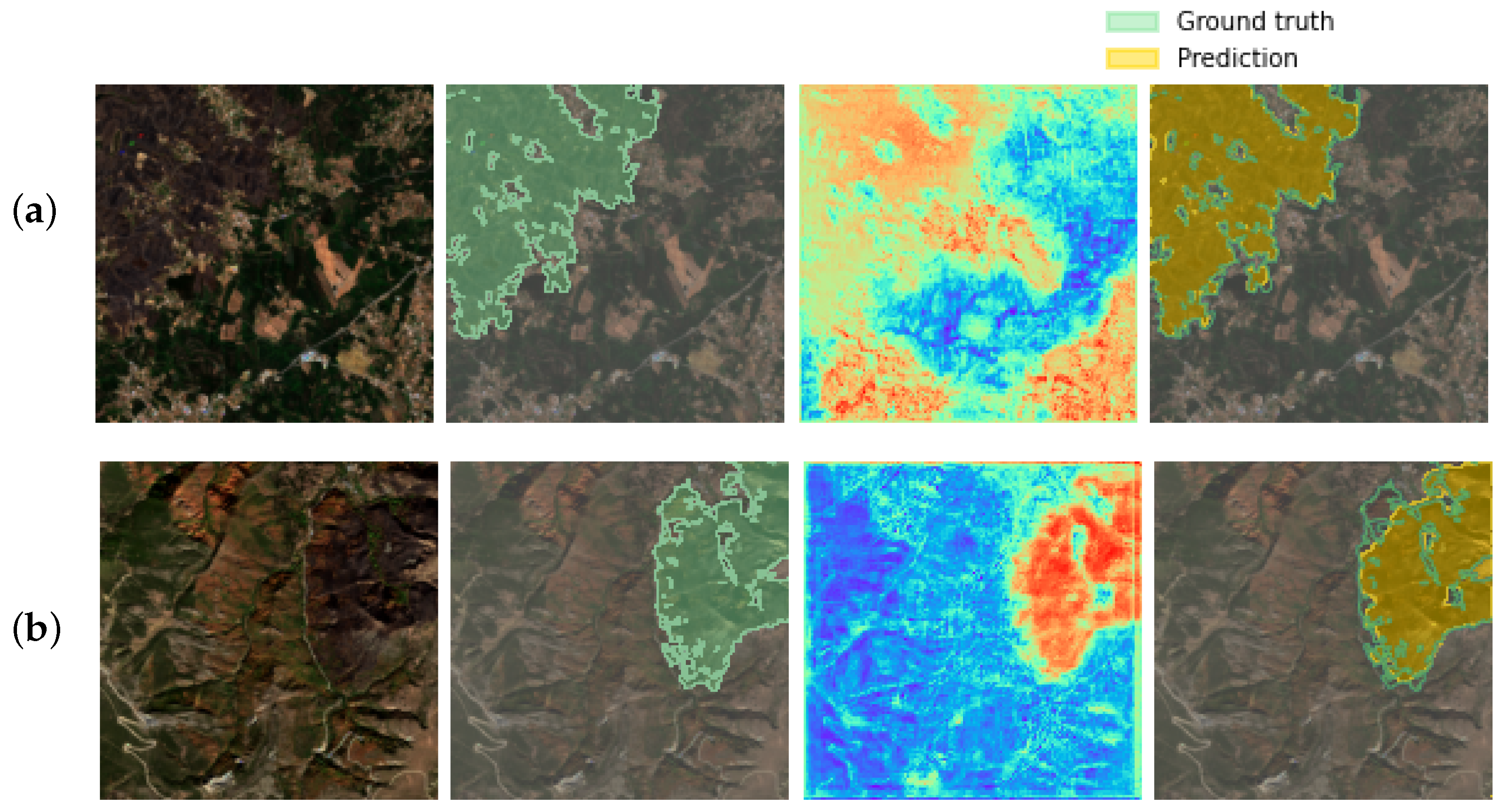
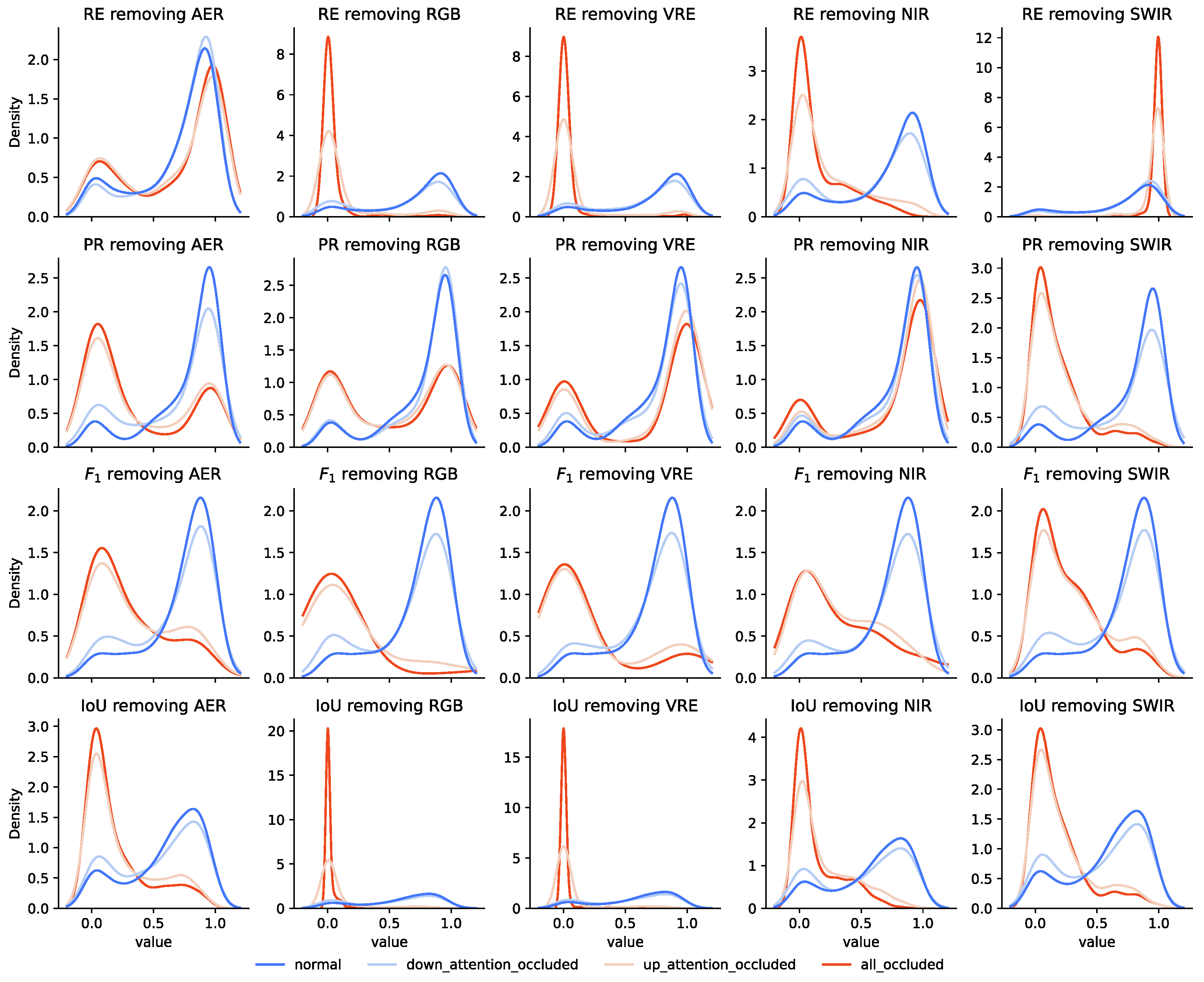
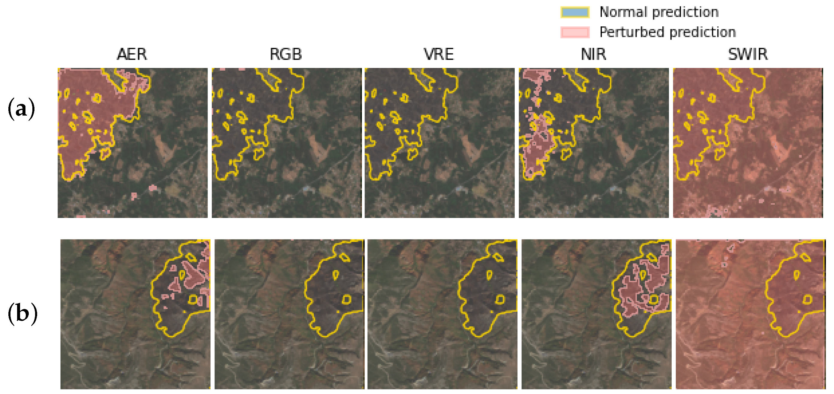
4.6. Multi-Channel Attention-Based Analysis

To address the interpretability of the trained models, in the following we focus on a multi-channel analysis of the DS-AttU architecture. All the following evaluations refer to the attention-based model trained with the BCE-MSE·F₁ losses. As shown in the previous sections, the AttentionUNet backbone is characterized by the presence of some attention layers in different points of the architecture. These components are built in such a way as to allow the detection of the areas in which the network is concentrating the most attention. The patterns of model attention can drive the investigation of the correctness of the learning process of the model. Even though the DS-AttU presents four attention layers for each backbone, we concentrate our analyses on the last layer. In this way, we intend to investigate the most complete set of information the network gets before making the final prediction.

Two examples of binary-class backbone output with the relative attention map are shown in Figure 5. The attention map is shown in the third column. Red pixels highlight higher values, while blue pixels highlight lower values of attention. Figure 5a shows that the attention layer output emphasizes a region that is larger than the final prediction, recalling that this mechanism has to be intended as a correlated but different process with respect to the actual network output. In the following, we inspect such a process to find relations to the network input and the resulting performance.

We know from domain experts that not all the 12 channels of Sentinel-2 L2A input images share the same importance in wildfire detection. An ideal solution should focus its attention both on the right position and on the most relevant input channels. Moreover, satellite channels carry information depending on the central wavelength they are sensible at. Therefore, it could be misleading to consider each channel separately since they can be grouped using the associated spectral bands. Particularly regarding wildfire detection, the work in [79] shows how reflectance in vegetation zones presents peaks separating the electromagnetic spectrum, as the satellite channels, into peculiar ranges. From these considerations, we propose to analyze the channels’ impact on the network by considering them grouped into domain-driven macro-bands as reported in

Table 3. Band aggregations following the common responses to terrain bodies.

Group	Sentinel-2 L2A Band	Central Wavelength (nm)
AER	Band 1—Coastal aerosol	442.7
RGB	Band 2—Blue	492.4
	Band 3—Green	559.8
	Band 4—Red	664.6
VRE	Band 5—Vegetation red edge	704.1
	Band 6—Vegetation red edge	740.5
	Band 7—Vegetation red edge	782.8
NIR	Band 8—NIR	832.8
	Band 8A—Narrow NIR	864.7
	Band 9—Water vapour	945.1
SWIR	Band 11—SWIR	1613.7
	Band 12—SWIR	2202.4

.

The first group (AER) consists of Band 1, which is generally used for analysis on water bodies [80] and atmosphere. Even though its central wavelength is close to bands 2, 3, and 4, we consider Band 1 in a separate group, as it is not in the range of visible wavelengths. The three RGB channels are the only ones in the human-eye visible range. They recall, with different order, the usual 3 channels of an RGB image, thus the name of the second group. The third multi-band collects all the channels in the Vegetation Red Edge (VRE) range, which is a Near-Infrared region characterized by a rapid change in reflectance of vegetation. Then, the fourth group collects the other Near-Infrared (NIR) channels and the band 9. Finally, the last group collects the remaining channels in the Short-Wave Infrared (SWIR) region.

To investigate the network’s ability to identify the most significant features, we performed a new test pipeline, alternatively presenting to the trained network input images obtained after an occlusion-perturbation process of some portions: such portions of the image are set to zero for each group of channels. We chose zero as perturbation value because it was already used in case of unavailable or invalid data: in the case of missing data from satellites, invalid pixels were encoded with zeros. Furthermore, such encoding is also used by the binary-class backbone, which masks the identified non-burned areas with zero-valued pixels. Hence, the usage of zero-valued pixels for the occlusion-perturbation mechanism in the analysis of the attention-guided explainability is motivated by the pre-existing encoding of invalid and to-be-ignored pixels.

Specifically, we applied three different types of perturbations:

• The all_occlusion perturbation sets to zero all the pixels belonging to the given macro-band group (i.e., all its channels/bands).
• The up_attention_occlusion perturbation sets to zero all the pixels belonging to the given macro-band and with an attention value greater than a defined threshold.
• The down_attention_occlusion perturbation, instead, sets to zero all the pixels belonging to the given macro-band and with an attention value lower than a defined threshold.

For instance, for the RGB Group, the all_occlusion perturbation sets to 0 all the pixels of the R, G, B channels; the up_attention_occlusion perturbation only the pixels of the R, G, B channels with attention greater than the threshold; and down_attention_occlusion perturbation only the pixels of the R, G, B channels with attention lower than the threshold (for all inputs in the dataset). The process is repeated and produces a new perturbed version of the dataset for each group and for each perturbation type.

The model’s performance on the entire original dataset is compared with each perturbed version of the dataset and may be affected by the perturbation in one of the following cases:

• If the performance decreases, the perturbation negatively affected the model, and therefore the original perturbed inputs were positively impacting on the original correct model’s predictions.
• If the performance remains the same, the perturbed inputs were neutral for the model.
• Finally, if the performance increases, the perturbed inputs were negatively impacting the model’s behavior on the original inputs.

We expect that the most relevant macro-bands groups would significantly affect performance as they are supposed to be fundamental in the prediction. In contrast, the least significant macro-bands groups would not considerably affect performance. Finally, if the perturbation of some macro-bands groups will increase the performance, then the model learned some pattern related to those groups incorrectly.

Moreover, we expect that a totally unreliable attention layer would present comparable performance when excluding high-attention and low-attention zones. Instead, an effective attention layer would be associated with a moderate loss in performance between the original images and the ones obtained by removing low-attention points and a high loss in performance between the original images and the ones with the perturbation of high-attention points.

In the following, we apply this strategy to the DS-AttU with the best loss configuration. While this procedure can be used for all four attention levels of the network, we decided to analyze the last one for each of the backbones, expecting that such positions would reflect the highest single-network degree of learning. Then, the high-low attention threshold has been selected by looking at the median value of the distribution of all the values of the attention feature maps get when spanning all the dataset images. Despite the two layers present different median distributions, as shown in Figure 6, we decide to fix a single threshold for both. As the second network result depends on the first one, we chose this value as the binary-class backbone distribution median, namely 0.43.

Finally, Figure 7 reports the binary step results. As for performance evaluation metrics, Recall, Precision, F1 score, and IoU were used for the binary classification step. Each plot represents the distribution of the results compared when using normal images, full-channel occlusion ones (marked as all_occluded) and the ones obtained by removing the high-attention (up_attention_occluded) and the low-attention points (down_attention_occluded). A detailed discussion is provided in Section 4.6.1.

To measure the channel’s relevance in the attention-guided prediction, we also evaluate the distance between the results distributions obtained considering the up- and down-threshold pixels. We focus this analysis on the first step of the architecture because the second step’s results strongly depend on the first network’s performance. To this aim, we can define P as the probability distribution associated with the results in terms of IoU obtained from the neural network without occlusions in the input. Analogous distributions trying to approximate the first one after a loss of information would be the ones obtained after the up_attention, down_attention, and all occlusions, which we can define as $Q^{+}$, $Q^{-}$ and $Q^{\mathrm{all}}$. To quantify the distance between them, we can introduce the Kullback–Leibler divergence ${\mathrm{D}}_{\mathrm{KL}}$, which is usually adopted in information theory and mathematical statistics to evaluate the distance between a real data probability distribution P and its approximation Q [81]. This metric, given the distributions P, Q and the associated densities $p\left(x\right)$, $q\left(x\right)$ with domain $\chi$, is defined as

$${\mathrm{D}}_{\mathrm{KL}}\left(P\right|\left|Q\right)={\int }_{\chi }dxp\left(x\right)log\left(\frac{p\left(x\right)}{q\left(x\right)}\right).$$

(1)

In our case, the density functions $p\left(x\right)$ and $q^{*}\left(x\right)$ (where * stays for all, up and down) can be estimated from the discrete samples using Kernel density estimation (KDE) algorithm. The domain of the functions derived in this way is ideally the set of all the real values, but we know that metrics generated from the confusion matrix can assume values from 0 to 1. Therefore, the densities are negligible when evaluated far from this range and we can truncate them. For this reason, all the integrals are evaluated between the aforementioned values with padding of half of the distance between the left and right limit on both sides, obtaining for the first step of the double-step analysis ${\chi }_{\mathrm{bin}}=x\in [-0.5,1.5]$.

Finally, starting from the ${\mathrm{D}}_{\mathrm{KL}}$, which by definition is always greater or equal to 0, we can derive a metric to evaluate the goodness of the attention layer as the variation between this metric calculated when removing the high- and down-attention pixels, namely,

$$\begin{array}{cc}\hfill \Delta {\mathrm{D}}_{\mathrm{KL}}& ={\mathrm{D}}_{\mathrm{KL}}\left(P\right||Q^{+})-{\mathrm{D}}_{\mathrm{KL}}\left(P\right||Q^{-})\hfill \\ \hfill & ={\int }_{x}dxp\left(x\right)log\left(\frac{p\left(x\right)}{q^{+}\left(x\right)}\right)-{\int }_{x}dxp\left(x\right)log\left(\frac{p\left(x\right)}{q^{-}\left(x\right)}\right)\hfill \\ \hfill & ={\int }_{x}dxp\left(x\right)log\left(\frac{q^{-}\left(x\right)}{q^{+}\left(x\right)}\right).\hfill \end{array}$$

(2)

As we assume a greater distance between $Q^{+}$ and P than between the down counterpart, we want this metric to be greater or equal to one for an effective attention layer. In the following sections, we present the results of this analysis for the first Backbone network and the direct consequences on the second one.

4.6.1. Binary Backbone

The plots shown in Figure 7 collect the results of the occlusion strategy described in the previous section, applied to the last level of the binary-class backbone. Every row of the graph represents the comparison between the performance distributions in terms of Recall (RE), Precision (PR), ${\mathrm{F}}_1$ Score, and Intersection over Union (IoU). The analysis is repeated for each channel group as the column changes.

Table 4. Divergences for the ${\mathrm{F}}_1$ score distributions. The first column shows the difference between the up- and down-attention occlusion as in Equation (3). The other ones are the values are the ${\mathrm{D}}_{\mathrm{KL}}\left(P\right||Q^{*})$ where ∗ stays for −, + and all.

Multi-Band	$\mathit{\delta }{\mathrm{D}}_{\mathbf{KL}}$	${\mathrm{D}}_{\mathbf{KL}}^{-}$	${\mathrm{D}}_{\mathbf{KL}}^{+}$	${\mathrm{D}}_{\mathbf{KL}}^{\mathbf{all}}$
AER	0.75	0.02	0.64	0.83
RGB	0.60	0.04	1.36	2.19
VRE	0.73	0.03	0.97	1.30
NIR	0.81	0.04	0.74	0.87
SWIR	0.78	0.03	0.95	1.17

collects instead the ${\mathrm{D}}_{\mathrm{KL}}$ of the ${\mathrm{F}}_1$ score distribution for the three occlusion alternatives and a normalized version of the $\Delta {\mathrm{D}}_{\mathrm{KL}}$, normalized with respect to the ${\mathrm{D}}_{\mathrm{KL}}^{\mathrm{all}}$ for the different channel groups. This last parameter is presented in order to investigate the effect of the attention-guided perturbation in terms of the maximum divergence of the group. The resulting measure is then calculated as the ratio

$$\delta {\mathrm{D}}_{\mathrm{KL}}=\frac{\Delta {\mathrm{D}}_{\mathrm{KL}}}{{\mathrm{D}}_{\mathrm{KL}}^{\mathrm{all}}}.$$

(3)

From these results, we can state that the less relevant Multi-band is AER, as it gets the lowest value of ${\mathrm{D}}_{\mathrm{KL}}^{\mathrm{all}}$ in terms of ${\mathrm{F}}_1$ score. Looking at the Recall distribution, we observe that the all_occluded distribution is particularly close to the normal one. This indicates that most of the detected burnt pixels are preserved after the perturbation. The worsening of the Precision curve shows instead that the unburnt pixel detection ability is not preserved. Then we could say that the network without the AER band tends to identify more wildfires than with the full information, resulting in an overall decreasing in performance as shown in ${\mathrm{F}}_1$ score and IoU distributions.

Moving to the RGB Multi-band, it appears as the most significant one, as the ${\mathrm{D}}_{\mathrm{KL}}^{\mathrm{all}}$ presents the maximum value among the groups. The associated Recall curve, which is highly peaked at 0, suggests that most of the wildfires are not detected anymore with this kind of perturbation. On the other side, as shown in the Precision curve, the degradation is not mitigated by the detection of 0-labeled pixels, then a general prediction in this way would probably present a high number of unburnt pixels and most of the burnt ones pointing to wrong areas. In contrast with the significance of the Multi-band, we can also observe that the $\delta {\mathrm{D}}_{\mathrm{KL}}$ is the lowest among the resulting values. Therefore, the network selects these channels as relevant information, as shown by the absolute values of the single divergences, but a higher focus is probably given to other groups.

VRE and NIR present similar trends with respect to each other and, still having slightly better performance, to the previous one. Therefore, we again expect a general prediction with a higher presence of correctly identified unburnt pixels than burnt ones. Anyway, this degradation is less pronounced when perturbing the NIR group in both the Precision and the Recall performance.

Finally, the perturbation on the SWIR channels ends up in a reversed scenario, in which the precision drastically decrease, but this happens in association with a significant improvement of the Recall. This trend can be explained if the network identifies as burnt almost every pixel of the perturbed images. As a last remark, Table 4 shows that the highest $\delta {\mathrm{D}}_{\mathrm{KL}}$ values appears for NIR and SWIR Multi-bands. Even though they are not the most relevant groups after the all-occlusion perturbation, this is an interesting result, as both bands composing the NBR index (namely, 8 and 12) came from these spectral ranges. Then, regarding the wildfire delineation phase, the network attention is effectively watching where a domain expert would have looked at.

The interpretations of the results as the perturbed Multi-band changes is recalled in Figure 8, in which the input images are the same of Figure 5. In both the examples we can observe that removing AER, and NIR results in a limited performance loss with respect to the normal prediction (the yellow line in the figures). This observation is in accordance to domain knowledge, since AER channel is the less significant when analyzing the spectral response. Instead, predictions from the perturbation on the RGB, VRE, and SWIR groups are close to an all-unburnt and all-burnt maps, respectively.

4.6.2. Regression Backbone

Moving to the second step network, it is important to recall the network operation, in order to understand how the first backbone errors can affect the final computation. In particular, the second network input is obtained as the entering satellite image masked by the first network binary map. Therefore, when an input perturbation results in an empty mask, as a full-of-zeros middle input from the intermediate step, we could imagine that the outcoming regression prediction would be dominated by noise. In the previous section we observed that the predictions obtained by perturbing RGB and VRE Multi-bands is expected to present for most of the inputs such a situation. As shown in Figure 9, the final prediction in the proposed examples are again empty masks. On the other side, the SWIR channels occlusion ends up in an all-burnt prediction. This behavior could suggests that, even though the second network gets most of the input information after the first backbone masking, the missing channels are still necessary to perform the regression.

Summing up, the result obtained at the end of the second step is strongly related to the information shared through the first. Therefore the only occlusion operation we can expect to give acceptable results would be the AER and the NIR. The proposed examples effectively reproduce this effect.

5. Conclusions and Future Works

This paper presents an extensive experimental evaluation of a double-step CNN solution in predicting areas damaged by forest wildfires and their damage assessment without the need of pre-fire images. Experimental results on a very large real-world satellite dataset demonstrate the power of the Double-Step deep learning Framework: most of the proposed network-loss combinations obtain high-quality results across the whole dataset. The most performant DSF achieved an rMSE score of 1.30 on burnt classes, leading in the majority of cases to mean errors of one severity (neighboring) class, thus providing useful information for preliminary analyses of areas affected by wildfires through remote sensing images. We further emphasize the fact that the aforementioned rMSE value is computed considering only burnt regions.

The Attention-based network we introduced has been shown to maintain high performance in the prediction in association with the possibility to inspect the deep learning model’s behavior. Domain knowledge has been applied to aggregate the satellite input channels and investigate their effects on the network learning process. The multi-channel attention-based analysis allowed us to identify groups of channels with different importance with respect to the prediction task. To this aim, we also introduced an attention-based occlusion method to increase the network interpretability. This strategy allows a whole-dataset measure of the network attention strength. An extension to this procedure is the implementation of such layers to an image- or pixel-wise magnitude. This means the possibility to provide to domain experts both a prediction of the damaged region and a clearer explanation of the process the network made to give such a result.

Future directions of this work include a deeper use of the attention layer to enhance the final prediction and offer a clearer way to solve common errors in the detection. Additionally, the benefits of a multi-step compound model can be further analyzed by including domain knowledge on spectral bands and eventually build ensemble models to better exploit all the available information.

References

1. San-Miguel-Ayanz, J.; Durrant, T.; Boca, R.; Liberta, G.; Branco, A.; De Rigo, D.; Ferrari, D.; Maianti, P.; Artes Vivancos, T.; Pfeiffer, H.; et al. Forest Fires in Europe, Middle East and North Africa 2018; Publications Office of the European Union: Luxembourg, 2019. [Google Scholar] [CrossRef]
2. San-Miguel-Ayanz, J.; Durrant, T.; Boca, R.; Maianti, P.; Liberta, G.; Artes Vivancos, T.; Branco, A.; De Rigo, D.; Ferrari, D.; Pfieffer, H.; et al. Advance EFFIS Report on Forest Fires in Europe, Middle East and North Africa 2019; Publications Office of the European Union: Luxembourg, 2020. [Google Scholar] [CrossRef]
3. European Forest Fire Information System (EFFIS)—Annual Reports. 2019. Available online: https://effis.jrc.ec.europa.eu/reports-and-publications/annual-fire-reports (accessed on 28 September 2021).
4. Euronews. 2019. Available online: https://www.euronews.com/2019/08/15/there-have-been-three-times-more-wildfires-in-the-eu-so-far-this-year (accessed on 28 September 2021).
5. Santopaolo, A.; Saif, S.S.; Pietrabissa, A.; Giuseppi, A. Forest Fire Risk Prediction from Satellite Data with Convolutional Neural Networks. In Proceedings of the 2021 29th Mediterranean Conference on Control and Automation (MED), Puglia, Italy, 22–25 June 2021; pp. 360–367. [Google Scholar]
6. Lestari, A.I.; Luhurkinanti, D.L.; Fitriasari, H.I.; Harwahyu, R.; Sari, R.F. Machine learning approaches for burned area identification using Sentinel-2 in Central Kalimantan. J. Appl. Eng. Sci. 2020, 18, 207–215. [Google Scholar]
7. Wittenberg, L. Post-fire soil erosion–the Mediterranean perception. In Pines and Their Mixed Forest Ecosystems in the Mediterranean Basin; Springer: Berlin/Heidelberg, Germany, 2021; pp. 481–496. [Google Scholar]
8. Chuvieco, E.; Mouillot, F.; van der Werf, G.R.; San Miguel, J.; Tanase, M.; Koutsias, N.; García, M.; Yebra, M.; Padilla, M.; Gitas, I.; et al. Historical background and current developments for mapping burned area from satellite Earth observation. Remote Sens. Environ. 2019, 225, 45–64. [Google Scholar] [CrossRef]
9. Klein, T.; Cahanovitc, R.; Sprintsin, M.; Herr, N.; Schiller, G. A nation-wide analysis of tree mortality under climate change: Forest loss and its causes in Israel 1948–2017. For. Ecol. Manag. 2019, 432, 840–849. [Google Scholar] [CrossRef]
10. Vaglio Laurin, G.; Francini, S.; Luti, T.; Chirici, G.; Pirotti, F.; Papale, D. Satellite open data to monitor forest damage caused by extreme climate-induced events: A case study of the Vaia storm in Northern Italy. For. Int. J. For. Res. 2021, 94, 407–416. [Google Scholar] [CrossRef]
11. Khryashchev, V.; Larionov, R. Wildfire Segmentation on Satellite Images using Deep Learning. In Proceedings of the 2020 Moscow Workshop on Electronic and Networking Technologies (MWENT), Moscow, Russia, 11–13 March 2020; pp. 1–5. [Google Scholar]
12. Farasin, A.; Colomba, L.; Palomba, G.; Nini, G.; Rossi, C. Supervised Burned Areas delineation by means of Sentinel-2 imagery and Convolutional Neural Networks. In Proceedings of the 17th International Conference on Information Systems for Crisis Response and Management (ISCRAM 2020), Virginia Tech, Blacksburg, VA, USA, 23–26 May 2020; pp. 24–27. [Google Scholar]
13. Knopp, L.; Wieland, M.; Rättich, M.; Martinis, S. A deep learning approach for burned area segmentation with Sentinel-2 data. Remote Sens. 2020, 12, 2422. [Google Scholar] [CrossRef]
14. Loboda, T.; O’Neal, K.; Csiszar, I. Regionally adaptable dNBR-based algorithm for burned area mapping from MODIS data. Remote Sens. Environ. 2007, 109, 429–442. [Google Scholar] [CrossRef]
15. Cicala, L.; Angelino, C.V.; Fiscante, N.; Ullo, S.L. Landsat-8 and Sentinel-2 for fire monitoring at a local scale: A case study on Vesuvius. In Proceedings of the 2018 IEEE International Conference on Environmental Engineering (EE), Delhi, India, 11–13 March 2018; pp. 1–6. [Google Scholar] [CrossRef]
16. Miller, J.D.; Thode, A.E. Quantifying burn severity in a heterogeneous landscape with a relative version of the delta Normalized Burn Ratio (dNBR). Remote Sens. Environ. 2007, 109, 66–80. [Google Scholar] [CrossRef]
17. Llorens, R.; Sobrino, J.A.; Fernández, C.; Fernández-Alonso, J.M.; Vega, J.A. A methodology to estimate forest fires burned areas and burn severity degrees using Sentinel-2 data. Application to the October 2017 fires in the Iberian Peninsula. Int. J. Appl. Earth Obs. Geoinf. 2021, 95, 102243. [Google Scholar] [CrossRef]
18. Gao, B.C. NDWI—A normalized difference water index for remote sensing of vegetation liquid water from space. Remote Sens. Environ. 1996, 58, 257–266. [Google Scholar] [CrossRef]
19. Rouse, J.W.; Haas, R.H.; Schell, J.A.; Deering, D.W. Monitoring vegetation systems in the Great Plains with ERTS. NASA Spec. Publ. 1974, 351, 309. [Google Scholar]
20. Filipponi, F. BAIS2: Burned area index for Sentinel-2. Proceedings 2018, 2, 364. [Google Scholar] [CrossRef] [Green Version]
21. Van der Meer, F.; Van der Werff, H.; Van Ruitenbeek, F. Potential of ESA’s Sentinel-2 for geological applications. Remote Sens. Environ. 2014, 148, 124–133. [Google Scholar] [CrossRef]
22. Dkhala, B.; Mezned, N.; Gomez, C.; Abdeljaouad, S. Hyperspectral field spectroscopy and SENTINEL-2 Multispectral data for minerals with high pollution potential content estimation and mapping. Sci. Total Environ. 2020, 740, 140160. [Google Scholar] [CrossRef]
23. Salehi, S.; Mielke, C.; Brogaard Pedersen, C.; Dalsenni Olsen, S. Comparison of ASTER and Sentinel-2 spaceborne datasets for geological mapping: A case study from North-East Greenland. Geol. Surv. Den. Greenl. Bull. 2019, 43, e2019430205. [Google Scholar] [CrossRef]
24. Castaldi, F.; Hueni, A.; Chabrillat, S.; Ward, K.; Buttafuoco, G.; Bomans, B.; Vreys, K.; Brell, M.; van Wesemael, B. Evaluating the capability of the Sentinel 2 data for soil organic carbon prediction in croplands. ISPRS J. Photogramm. Remote Sens. 2019, 147, 267–282. [Google Scholar] [CrossRef]
25. Bin, W.; Ming, L.; Dan, J.; Suju, L.; Qiang, C.; Chao, W.; Yang, Z.; Huan, Y.; Jun, Z. A Method of Automatically Extracting Forest Fire Burned Areas Using Gf-1 Remote Sensing Images. In Proceedings of the IGARSS 2019–2019 IEEE International Geoscience and Remote Sensing Symposium, Yokohama, Japan, 28 July–2 August 2019; pp. 9953–9955. [Google Scholar] [CrossRef]
26. Otsu, N. A Threshold Selection Method from Gray-Level Histograms. IEEE Trans. Syst. Man Cybern. 1979, 9, 62–66. [Google Scholar] [CrossRef] [Green Version]
27. Sezgin, M.; Sankur, B. Survey over image thresholding techniques and quantitative performance evaluation. J. Electron. Imaging 2004, 13, 146–165. [Google Scholar] [CrossRef]
28. Roy, D.P.; Boschetti, L.; Trigg, S.N. Remote sensing of fire severity: Assessing the performance of the normalized burn ratio. IEEE Geosci. Remote Sens. Lett. 2006, 3, 112–116. [Google Scholar] [CrossRef] [Green Version]
29. Navarro, G.; Caballero, I.; Silva, G.; Parra, P.C.; Vázquez, Á.; Caldeira, R. Evaluation of forest fire on Madeira Island using Sentinel-2A MSI imagery. Int. J. Appl. Earth Obs. Geoinf. 2017, 58, 97–106. [Google Scholar] [CrossRef] [Green Version]
30. Fernández-Manso, A.; Quintano, C.; Roberts, D.A. Can Landsat-Derived Variables Related to Energy Balance Improve Understanding of Burn Severity From Current Operational Techniques? Remote Sens. 2020, 12, 890. [Google Scholar] [CrossRef] [Green Version]
31. Rapid Damage Assessment. 2019. Available online: https://effis.jrc.ec.europa.eu/about-effis/technical-background/rapid-damage-assessment (accessed on 28 September 2021).
32. Fernández-Manso, A.; Fernández-Manso, O.; Quintano, C. SENTINEL-2A red-edge spectral indices suitability for discriminating burn severity. Int. J. Appl. Earth Obs. Geoinf. 2016, 50, 170–175. [Google Scholar] [CrossRef]
33. Liu, M.; Popescu, S.; Malambo, L. Feasibility of burned area mapping based on ICESAT-2 photon counting data. Remote Sens. 2020, 12, 24. [Google Scholar] [CrossRef] [Green Version]
34. Key, C.H.; Benson, N.C. Landscape assessment (LA). In FIREMON: Fire Effects Monitoring and Inventory System; Lutes Duncan, C., Keane, R.E., Caratti, J.F., Key, C.H., Benson, N.C., Sutherland, S., Gangi, L.J., Eds.; Gen. Tech. Rep. RMRS-GTR-164-CD; U.S. Department of Agriculture, Forest Service, Rocky Mountain Research Station: Fort Collins, CO, USA, 2006; Volume 64, p. LA-1-55. [Google Scholar]
35. Hardtke, L.A.; Blanco, P.D.; del Valle, H.F.; Metternicht, G.I.; Sione, W.F. Semi-automated mapping of burned areas in semi-arid ecosystems using MODIS time-series imagery. Int. J. Appl. Earth Obs. Geoinf. 2015, 38, 25–35. [Google Scholar] [CrossRef]
36. Ramo, R.; Chuvieco, E. Developing a random forest algorithm for MODIS global burned area classification. Remote Sens. 2017, 9, 1193. [Google Scholar] [CrossRef] [Green Version]
37. Ban, Y.; Zhang, P.; Nascetti, A.; Bevington, A.R.; Wulder, M.A. Near Real-Time Wildfire Progression Monitoring with Sentinel-1 SAR Time Series and Deep Learning. Sci. Rep. 2020, 10, 1–15. [Google Scholar] [CrossRef] [PubMed] [Green Version]
38. Pinto, M.M.; Libonati, R.; Trigo, R.M.; Trigo, I.F.; DaCamara, C.C. A deep learning approach for mapping and dating burned areas using temporal sequences of satellite images. ISPRS J. Photogramm. Remote Sens. 2020, 160, 260–274. [Google Scholar] [CrossRef]
39. Litjens, G.; Kooi, T.; Bejnordi, B.E.; Setio, A.A.A.; Ciompi, F.; Ghafoorian, M.; Van Der Laak, J.A.; Van Ginneken, B.; Sánchez, C.I. A survey on deep learning in medical image analysis. Med. Image Anal. 2017, 42, 60–88. [Google Scholar] [CrossRef] [Green Version]
40. Chen, H.; Qi, X.; Yu, L.; Heng, P.A. DCAN: Deep contour-aware networks for accurate gland segmentation. In Proceedings of the IEEE Conference on Computer Vision and Pattern Recognition, Las Vegas, NV, USA, 27–30 June 2016; pp. 2487–2496. [Google Scholar]
41. Gabruseva, T.; Poplavskiy, D.; Kalinin, A. Deep Learning for Automatic Pneumonia Detection. In Proceedings of the IEEE/CVF Conference on Computer Vision and Pattern Recognition (CVPR) Workshops, Seattle, WA, USA, 14–19 June 2020. [Google Scholar]
42. Ronneberger, O.; Fischer, P.; Brox, T. U-net: Convolutional Networks for Biomedical Image Segmentation. In International Conference on Medical Image Computing and Computer-Assisted Intervention; Springer: Berlin/Heidelberg, Germany, 2015; pp. 234–241. [Google Scholar]
43. Li, H.; Wang, C.; Cui, Y.; Hodgson, M. Mapping salt marsh along coastal South Carolina using U-Net. ISPRS J. Photogramm. Remote Sens. 2021, 179, 121–132. [Google Scholar] [CrossRef]
44. Cao, K.; Zhang, X. An improved res-unet model for tree species classification using airborne high-resolution images. Remote Sens. 2020, 12, 1128. [Google Scholar] [CrossRef] [Green Version]
45. Jiao, L.; Huo, L.; Hu, C.; Tang, P. Refined UNet: UNet-Based refinement network for cloud and shadow precise segmentation. Remote Sens. 2020, 12, 2001. [Google Scholar] [CrossRef]
46. Rashkovetsky, D.; Mauracher, F.; Langer, M.; Schmitt, M. Wildfire Detection from Multisensor Satellite Imagery Using Deep Semantic Segmentation. IEEE J. Sel. Top. Appl. Earth Obs. Remote Sens. 2021, 14, 7001–7016. [Google Scholar] [CrossRef]
47. Badrinarayanan, V.; Kendall, A.; Cipolla, R. Segnet: A deep convolutional encoder-decoder architecture for image segmentation. IEEE Trans. Pattern Anal. Mach. Intell. 2017, 39, 2481–2495. [Google Scholar] [CrossRef] [PubMed]
48. Chen, L.C.; Papandreou, G.; Schroff, F.; Adam, H. Rethinking atrous convolution for semantic image segmentation. arXiv 2017, arXiv:1706.05587. [Google Scholar]
49. Zhao, H.; Shi, J.; Qi, X.; Wang, X.; Jia, J. Pyramid scene parsing network. In Proceedings of the IEEE Conference on Computer Vision and Pattern Recognition, Honolulu, HI, USA, 21–26 July 2017; pp. 2881–2890. [Google Scholar]
50. Farasin, A.; Colomba, L.; Garza, P. Double-Step U-Net: A Deep Learning-Based Approach for the Estimation of Wildfire Damage Severity through Sentinel-2 Satellite Data. Appl. Sci. 2020, 10, 4332. [Google Scholar] [CrossRef]
51. Monaco, S.; Pasini, A.; Apiletti, D.; Colomba, L.; Garza, P.; Baralis, E. Improving Wildfire Severity Classification of Deep Learning U-Nets from Satellite Images. In Proceedings of the 2020 IEEE International Conference on Big Data (Big Data), Atlanta, GA, USA, 10–13 December 2020; pp. 5786–5788. [Google Scholar]
52. Ciprián-Sánchez, J.F.; Ochoa-Ruiz, G.; Rossi, L.; Morandini, F. Assessing the Impact of the Loss Function, Architecture and Image Type for Deep Learning-Based Wildfire Segmentation. Appl. Sci. 2021, 11, 7046. [Google Scholar] [CrossRef]
53. Jadon, S.; Leary, O.P.; Pan, I.; Harder, T.J.; Wright, D.W.; Merck, L.H.; Merck, D.L. A comparative study of 2D image segmentation algorithms for traumatic brain lesions using CT data from the ProTECTIII multicenter clinical trial. In Medical Imaging 2020: Imaging Informatics for Healthcare, Research, and Applications; International Society for Optics and Photonics: Bellingham, WA, USA, 2020; Volume 11318, p. 113180Q. [Google Scholar]
54. Monaco, S.; Pasini, A.; Apiletti, D.; Colomba, L.; Farasin, A.; Garza, P.; Baralis, E. Double-Step deep learning framework to improve wildfire severity classification. In Proceedings of the Workshops of the EDBT/ICDT 2021 Joint Conference, Nicosia, Cyprus, 23 March 2021; Volume 2841. [Google Scholar]
55. Guidotti, R.; Monreale, A.; Ruggieri, S.; Turini, F.; Giannotti, F.; Pedreschi, D. A Survey of Methods for Explaining Black Box Models. ACM Comput. Surv. 2018, 51, 1–42. [Google Scholar] [CrossRef] [Green Version]
56. Selvaraju, R.R.; Cogswell, M.; Das, A.; Vedantam, R.; Parikh, D.; Batra, D. Grad-CAM: Visual Explanations from Deep Networks via Gradient-Based Localization. In Proceedings of the 2017 IEEE International Conference on Computer Vision (ICCV), Venice, Italy, 22–29 October 2017; pp. 618–626. [Google Scholar] [CrossRef] [Green Version]
57. Chattopadhay, A.; Sarkar, A.; Howlader, P.; Balasubramanian, V.N. Grad-CAM++: Generalized Gradient-Based Visual Explanations for Deep Convolutional Networks. In Proceedings of the 2018 IEEE Winter Conference on Applications of Computer Vision (WACV), Lake Tahoe, NV, USA, 12–15 March 2018; pp. 839–847. [Google Scholar] [CrossRef] [Green Version]
58. Zhou, B.; Khosla, A.; Lapedriza, A.; Oliva, A.; Torralba, A. Learning Deep Features for Discriminative Localization. In Proceedings of the 2016 IEEE Conference on Computer Vision and Pattern Recognition (CVPR), Las Vegas, NV, USA, 27–30 June 2016; pp. 2921–2929. [Google Scholar] [CrossRef] [Green Version]
59. Zeiler, M.D.; Fergus, R. Visualizing and Understanding Convolutional Networks. arXiv 2013, arXiv:1311.2901. [Google Scholar]
60. Simonyan, K.; Vedaldi, A.; Zisserman, A. Deep Inside Convolutional Networks: Visualising Image Classification Models and Saliency Maps. arXiv 2014, arXiv:1312.6034. [Google Scholar]
61. Springenberg, J.T.; Dosovitskiy, A.; Brox, T.; Riedmiller, M. Striving for Simplicity: The All Convolutional Net. arXiv 2015, arXiv:1412.6806. [Google Scholar]
62. Ribeiro, M.T.; Singh, S.; Guestrin, C. “Why Should I Trust You?”: Explaining the Predictions of Any Classifier. In Proceedings of the 22nd ACM SIGKDD International Conference on Knowledge Discovery and Data Mining, San Francisco, CA, USA, 13–17 August 2016; Association for Computing Machinery: New York, NY, USA, 2016; pp. 1135–1144. [Google Scholar] [CrossRef]
63. Ventura, F.; Cerquitelli, T.; Giacalone, F. Black-Box Model Explained Through an Assessment of Its Interpretable Features. In New Trends in Databases and Information Systems; Benczúr, A., Thalheim, B., Horváth, T., Chiusano, S., Cerquitelli, T., Sidló, C., Revesz, P.Z., Eds.; Springer International Publishing: Cham, Switzerland, 2018. [Google Scholar]
64. Shapley, L.S. A value for n-person games. Contrib. Theory Games 1953, 2, 307–317. [Google Scholar]
65. Schorr, C.; Goodarzi, P.; Chen, F.; Dahmen, T. Neuroscope: An Explainable AI Toolbox for Semantic Segmentation and Image Classification of Convolutional Neural Nets. Appl. Sci. 2021, 11, 2199. [Google Scholar] [CrossRef]
66. Ma, J. Segmentation Loss Odyssey. arXiv 2020, arXiv:2005.13449. [Google Scholar]
67. Zhou, Z.; Siddiquee, M.M.R.; Tajbakhsh, N.; Liang, J. Unet++: A nested u-net architecture for medical image segmentation. In Deep Learning in Medical Image Analysis and Multimodal Learning for Clinical Decision Support; Springer: Berlin/Heidelberg, Germany, 2018; pp. 3–11. [Google Scholar]
68. Kamal, U.; Tonmoy, T.I.; Das, S.; Hasan, M.K. Automatic traffic sign detection and recognition using SegU-Net and a modified Tversky loss function with L1-constraint. IEEE Trans. Intell. Transp. Syst. 2019, 21, 1467–1479. [Google Scholar] [CrossRef]
69. Badrinarayanan, V.; Handa, A.; Cipolla, R. Segnet: A deep convolutional encoder-decoder architecture for robust semantic pixel-wise labelling. arXiv 2015, arXiv:1505.07293. [Google Scholar]
70. Yakubovskiy, P. Segmentation Models Pytorch. 2020. Available online: https://github.com/qubvel/segmentation_models.pytorch (accessed on 28 September 2021).
71. Gu, R.; Wang, G.; Song, T.; Huang, R.; Aertsen, M.; Deprest, J.; Ourselin, S.; Vercauteren, T.; Zhang, S. CA-Net: Comprehensive attention convolutional neural networks for explainable medical image segmentation. IEEE Trans. Med. Imaging 2020, 40, 699–711. [Google Scholar] [CrossRef]
72. SentinelHub. Available online: https://www.sentinel-hub.com (accessed on 28 October 2021).
73. Xu, H. Modification of normalised difference water index (NDWI) to enhance open water features in remotely sensed imagery. Int. J. Remote Sens. 2006, 27, 3025–3033. [Google Scholar] [CrossRef]
74. Paszke, A.; Gross, S.; Massa, F.; Lerer, A.; Bradbury, J.; Chanan, G.; Killeen, T.; Lin, Z.; Gimelshein, N.; Antiga, L.; et al. Pytorch: An imperative style, high-performance deep learning library. Adv. Neural Inf. Process. Syst. 2019, 32, 8026–8037. [Google Scholar]
75. McKinney, W. Data Structures for Statistical Computing in Python. In Proceedings of the 9th Python in Science Conference, Austin, TX, USA, 28 June–3 July 2010; pp. 56–61. [Google Scholar] [CrossRef] [Green Version]
76. Harris, C.R.; Millman, K.J.; van der Walt, S.J.; Gommers, R.; Virtanen, P.; Cournapeau, D.; Wieser, E.; Taylor, J.; Berg, S.; Smith, N.J.; et al. Array programming with NumPy. Nature 2020, 585, 357–362. [Google Scholar] [CrossRef]
77. Hunter, J.D. Matplotlib: A 2D graphics environment. Comput. Sci. Eng. 2007, 9, 90–95. [Google Scholar] [CrossRef]
78. HPC@POLITO. 2019. Available online: https://hpc.polito.it/legion_cluster.php (accessed on 28 September 2021).
79. Candra, D.S. Deforestation detection using multitemporal satellite images. In IOP Conference Series: Earth and Environmental Science; IOP Publishing: Bristol, UK, 2020; Volume 500, p. 012037. [Google Scholar]
80. Poursanidis, D.; Traganos, D.; Reinartz, P.; Chrysoulakis, N. On the use of Sentinel-2 for coastal habitat mapping and satellite-derived bathymetry estimation using downscaled coastal aerosol band. Int. J. Appl. Earth Obs. Geoinf. 2019, 80, 58–70. [Google Scholar] [CrossRef]
81. Kullback, S.; Leibler, R.A. On information and sufficiency. Ann. Math. Stat. 1951, 22, 79–86. [Google Scholar] [CrossRef]
Figure 1. Double-Step deep learning Framework architecture.
Applsci 11 11060 g001
Figure 2. Loss function selection experiments. For each configuration (right column) the binary and regression losses are connected with a line of the same color.
Applsci 11 11060 g002
Figure 3. Visual representation of the Spatial Attention block of AttentionUNet.
Applsci 11 11060 g003
Figure 4. Distribution of the severity levels for each fold and globally. Unburnt pixels percentages are not shown and correspond to the complementary of the shown bars.
Applsci 11 11060 g004
Figure 5. Visualization of the last binary attention level compared to the network prediction. The first column is the RGB visualization of the input, the second is the binary ground truth, the third is the attention map (the intensity scale goes from blue to red for lower to higher attention values, respectively), while the last is the prediction. Rows (a) and (b) are two satellite examples from coral and cyan fold, respectively.
Applsci 11 11060 g005
Figure 6. Values distributions for each attention level of the regression backbone. The dashed lines represents the medians of the two distributions.
Applsci 11 11060 g006
Figure 7. Comparison of the binary prediction for each channel group between the normal case and the different occlusion strategies. The normal (blue line) distribution is the same for each row, while the y-scale is different across columns in order to fit the other curves.
Applsci 11 11060 g007
Figure 8. Visualization of the all_occlusion results for the different Multi-bands. Rows (a) and (b) are two satellite examples from coral and cyan fold, respectively.
Applsci 11 11060 g008
Figure 9. Visualization of the all_occlusion results for the different Multi-bands. Yellow contours indicate the severity scale region of the normal prediction. The perturbed prediction is indicated via the colored regions as in the legend.
Applsci 11 11060 g009