Article

Shallow S-Wave Velocity Structure in the Middle-Chelif Basin, Algeria, Using Ambient Vibration Single-Station and Array Measurements

by
Abdelouahab Issaadi
1,2,*,
Fethi Semmane
1,
Abdelkrim Yelles-Chaouche
1,
Juan José Galiana-Merino
2,3 and
Anis Mazari
1
1
Centre de Recherche en Astronomie Astrophysique et Géophysique (CRAAG), Algiers 16340, Algeria
2
University Institute of Physics Applied to Sciences and Technologies, University of Alicante, Crta. San Vicente del Raspeig, s/n, 03080 Alicante, Spain
3
Department of Physics, Systems Engineering, and Signal Theory, University of Alicante, Crta. San Vicente del Raspeig, s/n, 03080 Alicante, Spain
*
Author to whom correspondence should be addressed.
Appl. Sci. 2021, 11(22), 11058; https://doi.org/10.3390/app112211058
Submission received: 10 October 2021 / Revised: 18 November 2021 / Accepted: 19 November 2021 / Published: 22 November 2021
(This article belongs to the Special Issue Geohazards: Risk Assessment, Mitigation and Prevention)

Abstract

:
In order to better assess the seismic hazard in the northern region of Algeria, the shear-wave velocity structure in the Middle-Chelif Basin is estimated using ambient vibration single-station and array measurements. The Middle-Chelif Basin is located in the central part of the Chelif Basin, the largest of the Neogene sedimentary basins in northern Algeria. This basin hosts the El-Asnam fault, one of the most important active faults in the Mediterranean area. In this seismically active region, most towns and villages are built on large unconsolidated sedimentary covers. Application of the horizontal-to-vertical spectral ratio (HVSR) technique at 164 sites, and frequency–wavenumber (F–K) analysis at 7 other sites, allowed for the estimation of the ground resonance frequencies, shear-wave velocity profiles, and sedimentary cover thicknesses. The electrical resistivity tomography method was used at some sites to further constrain the thickness of the superficial sedimentary layers. The soil resonance frequencies range from 0.75 Hz to 12 Hz and the maximum frequency peak amplitude is 6.2. The structure of the estimated shear-wave velocities is presented in some places as 2D profiles to help interpret the existing faults. The ambient vibration data allowed us to estimate the maximum depth in the Middle-Chelif Basin, which is 760 m near the city of El-Abadia.

1. Introduction

Northern Algeria is characterized by a series of Neogene basins (e.g., Constantine Basin, Hodna Basin, Soummam Basin, Tizi-ouzou Basin, Mitidja Basin, Medea Basin, and Chelif Basin), elongated in an E–W direction, and surrounded by the Tellian Atlas mountain belts, which act as a substratum for their sedimentary covers [1,2,3]. These basins host important seismic activity, mainly in their marginal zones [4]. Active tectonics in the northern part of the country and the related seismicity are due to the fact that this zone is located at the boundary between the African and Eurasian convergent plates [4,5].
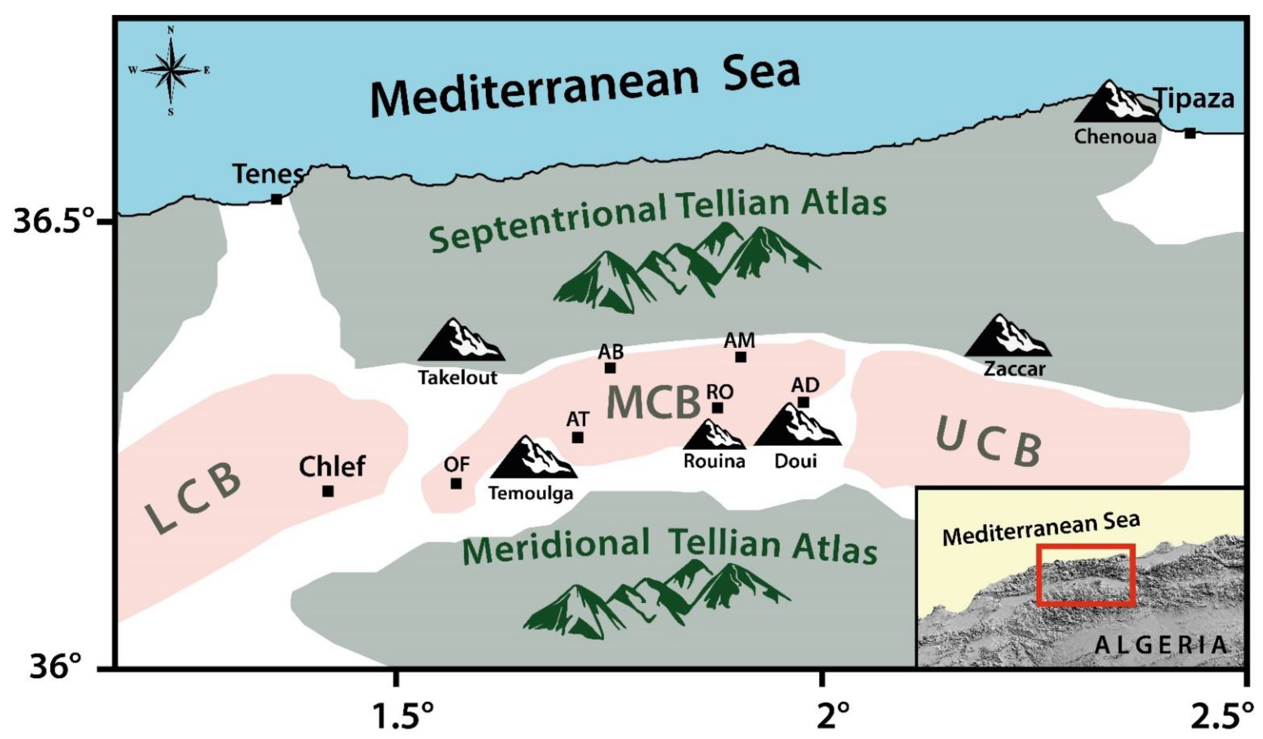
In the northwestern part of Algeria, between the septentrional and meridional Tellian Atlas mountain belts, lies the Chelif Basin, a wide depression of over 450 km in length, which is the largest and the most subsident of the sublittoral basins [2,3]. The dimensions of the basin and the complexity of its hydrographic network has led several authors to divide it into three sub-basins: The Lower-, the Middle-, and the Upper-Chelif. In this study, we focus on the plain extending from Oued-Fodda to Ain-Defla (Figure 1). However, one must note that this subdivision is not unanimous within the scientific community. While some authors assign our study area to the Middle-Chelif Basin [6,7,8], others have assigned it to the oriental part of the Lower-Chelif Basin [2,3,9]. In this study, we consider the study area as a part of the Middle-Chelif Basin.
The Middle-Chelif plain is home to over 400,000 inhabitants, who are mainly concentrated on its edges, and distributed over its principal cities, which are: Ain-Defla, Rouina, El-Amra, El-Attaf, El-Abadia, and Oued-Fodda.
The region has witnessed several destructive earthquakes, such as the 1858 El-Amra earthquake (I0 = IX, [10]); the 1934 El-Abadia earthquake (I0 = IX, [10]); the 1954 Orléansville earthquake (Ms 6.7, [10]); and the 1980 El-Asnam earthquake (Ms 7.3, [11]).
In the last few decades, techniques based on ambient vibrations have been widely used to study sedimentary basins because of the quick implementation and the lower cost of the process, compared to boreholes or other geophysical prospecting methods (e.g., [12,13,14,15,16]). It is proven that soft sedimentary layers can amplify the ground shaking and prolong its duration during an earthquake, which can be harmful for buildings. Therefore, the determination of the geotechnical characteristics of the soils is primary for seismic risk and site effects assessments. One of the most important parameters for determining the geotechnical characteristics is the shear-wave velocity structure. The high-velocity contrast between soft sediments and the bedrock, along with the local geological and topographical aspects, are important factors for ground motion amplification.
The Chelif Basin has been the subject of several geological and geophysical studies. The majority of these studies have been done on the Lower-Chelif Basin, and only a few of them have included the western part of the Middle-Chelif. It was only at the end of the 1960’s that the CGG (Compagnie Générale de Géophysique) carried out a geophysical prospecting campaign by electric methods in the Middle-Chelif Plain in order to study the structure of the sedimentary deposits [7].
Since the 1980 El-Asnam earthquake, and the damage it caused, the Middle-Chelif region has been the subject of a multitude of geological and geophysical studies. The first study was carried out by the Institute of Earthquake Engineering of Skopje University (Macedonia), which resulted in the elaboration of the code for the repairing and strengthening of damaged buildings in the Chelif region. The code was based on studies of seismic hazards and the geotechnical conditions of the soil. Several seismic refraction profiles were performed in the cities of Chlef and El-Attaf [17]. The Woodward Clyde Consultants also carried out a complete geotechnical and geological study in eight cities of the Chelif region, including Oued-Fodda, El-Attaf, and El-Abadia, where several boreholes were drilled. The study outcomes provided geotechnical and hydrogeological maps for each city, along with seismic microzoning survey maps [18]. The neotectonic and paleoseismological studies carried out on the formations of the oriental Lower-Chelif Basin (e.g., [9,19]) were intended to highlight the tectonic elements and to identify geological structures and faults likely to be reactivated by generating earthquakes.
More recently, site effects investigations using earthquakes and ambient vibration data were conducted in the cities of Chlef in the Lower-Chelif Basin [20,21] and Oued-Fodda in the Middle-Chelif Basin [22]. The main objectives were to estimate the soil resonance frequencies, the shear-wave velocities in the sedimentary rocks, and the depths to seismic bedrock, where the relatively high impedance contrast with Miocene formations may amplify ground shaking during an earthquake. In the Mitidja basin, Bouchelouh [23] and Tebbouche [24] estimated and mapped the roof of the engineering bedrock using mainly ambient vibration data.
In this study, ambient vibration measurements using single-station and array techniques were used to estimate the shear-wave velocity for the sedimentary layers, and to map the bedrock structure in the Middle-Chelif Basin. In the first part of the study, we estimate the soil resonance frequencies (f0) and the corresponding amplitudes (A0) using the horizontal-to-vertical spectral ratio (HVSR) technique [25,26]. In the second part, we perform array measurements using the frequency–wavenumber (F–K) technique [27,28,29,30] to retrieve the surface wave dispersion curves. After that, the dispersion and HVSR curves are inverted jointly to estimate the shear-wave velocity (Vs) profiles at each site. Available borehole information and electrical resistivity profiles constrain the Vs models used for the inversion process. As a result, the bedrock model is proposed.
This study is a continuation of previous work conducted in the city of Oued-Fodda [22]. The results obtained in this work will contribute to the seismic hazard reassessment in the Chelif Basin. They can also be used for seismic hazard mitigation studies, such as strong ground motion simulation, soil liquefaction studies, and for the updating of the Algerian seismic code.

2. Geological Framework

The Neogene basins, in the western part of Algeria, stretch parallel to the Mediterranean coast and lie within the septentrional and meridional Tellian Atlas mountain belts, which belong to the southern branch of the Alpine chain [1,31]. The intramountainous Chelif Basin is a wide depression of over 450 km filled with Mio-Plio-Quaternary deposits [1,2,3,9,32,33]. It is formed by a succession of plains, hills, and folds, boarded by the Dahra and Boumaad Mountains in the north, and the Ouarsenis Mountains in the south. These Tellian belts were structured during the Mesozoic [34] and constitute the substratum of the Neogene deposits.
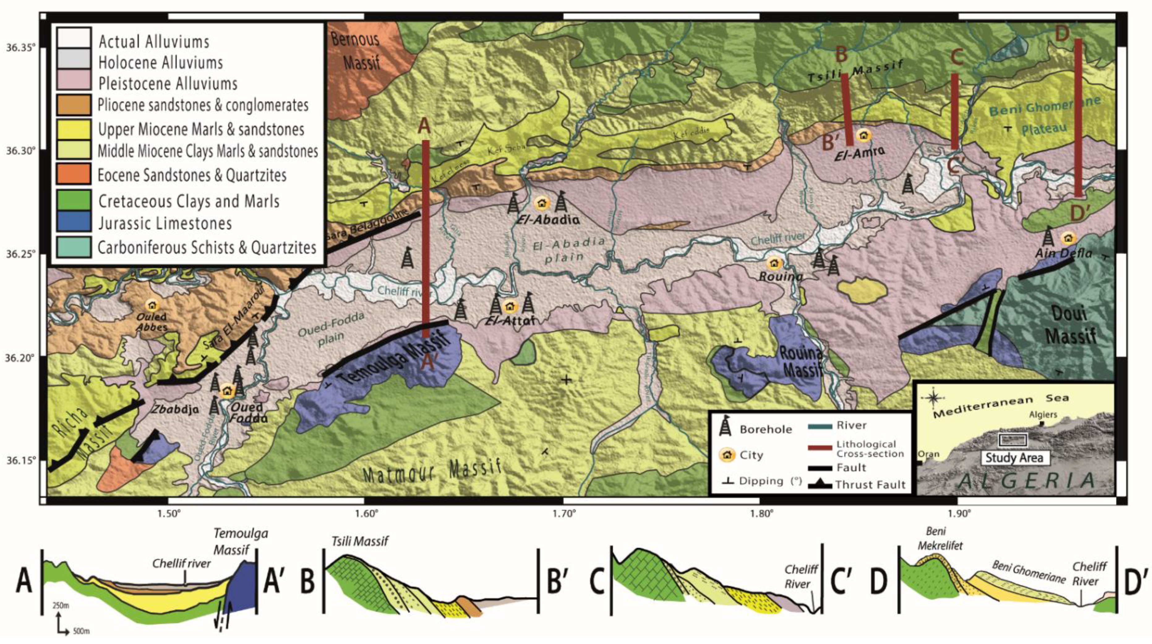
The Middle-Chelif Basin extends from the Sara-El-Maarouf anticline to the Beni-Ghomerian plateau (Figure 2). In its central part, the Quaternary plain forms a narrow strip that stretches for over 50 km. This region is affected by normal and thrust faults, including the so-called “El-Asnam Fault”. The orientation of these faults is parallel to the synclinal axis of the basin. The cross-sections performed by the National Society of Petroleum [35] and the General Company of Geophysics [7] show that the synclinal axis of this basin appears to be north of the Chelif River. In the southern part of this plain, inlier terrains of Jurassic-to-Silurian age outcrops form the Doui, Rouina, and Temoulga Massifs, from east to west, respectively. These schistosity massifs are considered to be autochthonous formations [33,34]. Although the Jurassic formations are predominant in these outcrops, the bedrock is mainly Cretaceous in most of the basin area, and it is composed of Cenomanian to Senonian clays and marls [36].
Several previous geological studies have detailed the lithological and stratigraphical aspect of the Neogene deposits in the Middle-Chelif Basin [2,9,32]. The first sedimentary deposit is a red detritic series of conglomerates, poudingues, and marls. Brives [32] and Perrodon [2] attribute these formations to the Lower Miocene, while Meghraoui [9] and Thomas [3] assign them to the Middle Miocene (Serravalo-Tortonian). These formations outcrop on the southern flank of the Tsili Massif, north of El-Amra (Figure 2). Above these formations lies an important intercalation of marls, clays, and limestones of the Lower Tortonian [9]. The boreholes and the electric surveying data used in this study [7] show that these formations can reach a considerable thickness of 400 m. This layer lies in discordance over the conglomeratic series in the northern part of the basin, and directly over the Cretaceous marls in the south. The passage between the Upper Tortonian sandstones and the Lower Tortonian marls is completed abruptly [32]. This contrast can be observed in Kef-Ensoura, north of El-Abadia, and also on the Beni-Ghomerian Plateau, where the two formations outcrop. The Messinian is represented mainly by blue marls with a maximum thickness of 50 m [9]. The marine regression in the Pliocene divided this stage into marine and continental formations [2,3,32]. The marine Pliocene is represented by sands and sandstones, while the continental is composed of red sands and conglomerates [2,9,32]. The Pliocene constitutes the principal deposits of the Sara-el-Maarouf and the Sara-Belaggoune anticlines, north of Oued-Fodda, and extends eastward by outcropping on a narrow band until the Beni-Ghomerian Plateau. However, this formation does not outcrop in the southern parts of the basin, which suggests that it disappears somewhere under the Quaternary plain. These deposits can reach a thickness of 200 m [9].
The Quaternary is predominant in the wide plain that stretches from Oued-Fodda to Ain-Defla. The Pleistocene formations surround the Holocene alluviums and form the first hills in the northern and southern margins of the plain. The Pleistocene is composed of clays, gravels, and conglomerates. The Holocene is constituted of recent alluviums. The Chelif River crosses the Middle-Chelif Quaternary Plain from Ain-Defla to Ouled-Abbes and drags all the necessary materials that form the actual alluviums.
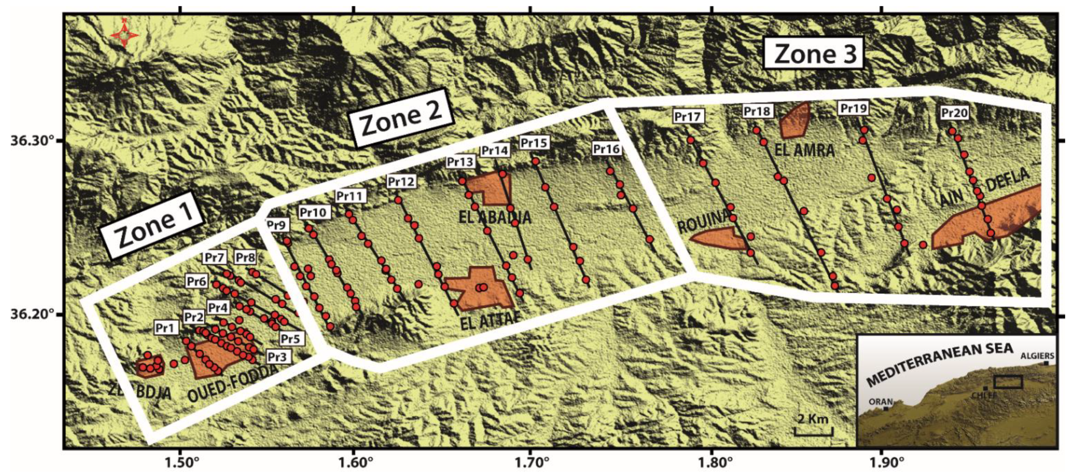
The geological and geotechnical data show important lateral variations in the facies and thicknesses within the sedimentary layers and the bedrock. For that, the study area was divided into three zones: The Oued-Fodda Plain, the Carnot Plain, and the Ain-Defla Region (Figure 3). The Oued-Fodda Plain lies between the Temoulga Massif and the Sara-El-Maarouf anticline in a NE–SW direction, with an average width of 3 km. The fault affecting the Temoulga Massif, east of the plain, and the El-Asnam fault in the west, suggest that this plain acts as a graben structure. The different outcrops in the area suggest a low sedimentary thickness [22]. The bedrock is mainly composed of Senonian marls.
The Carnot Plain, also known as the El-Attaf Plain, extends from Bir-Safsaf to Rouina in an E–W direction. The main cities of the plain are El-Attaf and El-Abadia, built on the southern and northern plain margins, respectively. The average basin width of 8 km suggests that the maximum depth of the basin is likely to be observed in this region. Lateral variations in the facies are observed in the Cretaceous series, which is considered as the bedrock of the sedimentary deposits in this area. The facies change from marly to mainly composed of limestones west of El-Abadia. The geophysical data show that the sedimentary layers can reach a depth of 700–800 m from El-Abadia to Rouina [6,7,35].

3. Methodology

3.1. The Horizontal-to-Vertical Ratio Technique

The HVSR technique (also known as H/V) was initiated by Nogoshi and Igarashi [26], and developed by Nakamura [25]. It is one of the most commonly used techniques that allows for the retrieval of one of the most important parameters of site response, i.e., the resonance frequency at a given site. This technique has proven its reliability in estimating the soil resonance frequency [37], although several authors have reported that this technique is not reliable in estimating the amplification factors, especially at lower frequencies [38,39,40,41]. This inability is due to the contribution of body and surface waves, and it is the latter ones that control the HVSR curve. The low contribution of body waves is sufficient for estimating the fundamental frequency, but not enough for estimating the amplification factor [38,39,41]. Recently, LaRocca [42] has also demonstrated how the peak amplitude of the HVSR of the seismic noise may vary considerably with time.
This method consists of estimating the ratio between the Fourier amplitude spectrum of the horizontal and vertical components of the ambient noise, which provides the HVSR curve as a result. The resulting HVSR frequency peak is very well-correlated with the resonance frequency of the soil [43]. This peak corresponds to an impedance contrast in the soil column.
The low cost, the simplicity of acquisition and processing, and the reliability in estimating the soil resonance frequencies, makes this technique one of the most used for site characterizations, especially for urban areas.

3.2. Inversion of the HVSR Curves

The inversion of the HVSR curves allows for the retrieval of the shear-wave velocity values for the sedimentary layers, along with the bedrock depths of our study area.
The velocity profiles are calculated using the neighborhood algorithm [44]. As there is no unique solution for the inversion problem, several velocity models are calculated. For each model, the calculated ellipticity of the Rayleigh wave fundamental mode is compared to the HVSR curve and a misfit value is given [45]. The ellipticity curves and the corresponding velocity models with the lower misfit values are considered.
As for all the inversion processes, the nonuniqueness of the solution is a very delicate matter to deal with, and hundreds of thousands of velocity models can result from one simple HVSR curve. For that reason, some soil parameters are required to better guide and constrain the process. The main parameter is the number of the sedimentary layers and the range of thicknesses for each layer. Geological or lithological cross-sections are usually good enough for providing these two parameters. Some geotechnical parameters are also required for each layer, either as fixed values or as intervals. These parameters are the Vp, Vs, density, and Poisson’s ratio. The latter is set between 0.2 and 0.5 (universal values for soils). For good and reliable results, it is necessary to have good data coverage in the study area, as well as boreholes and geophysical prospections (e.g., the seismic refraction experiment).

3.3. The Frequency–Wavenumber (F–K) Analysis

In the last decade, array-based techniques have become popular and are widely used for the analysis of ambient vibrations. The concept of configurations in arrays, with simultaneous ambient vibration recordings, has proven its reliability and efficiency through several studies and investigations [16,46,47]. One of the most applied techniques for array processing is frequency–wavenumber analysis, commonly known as F–K analysis [27,28,29,30]. This technique is performed in the frequency domain and allows for the estimation of the back azimuth and the slowness of the seismic wave sources recorded by the array [47].
The theoretical aspect of this technique is based on two main assumptions. The first one is that the wavefront propagation is on the vertical plane, and the process is stationary in the other two planes. The second assumption is that the process is stationary in time. The microtremor wavefield is a superposition of seismic waves propagated from several distant sources [28]. The F–K analysis exploits the stationary and stochastic character of these propagated waves to construct the frequency–wavenumber power spectral density function, which holds information on the power as a function of the frequency and the velocity of travelling waves. The power spectral density can be estimated using the following two following methods: The beam-forming method (BFM) [29,30], and the maximum likelihood method (MLM) or the high-resolution method (HR) [27,28,48]. In this study, we used the beam-forming method to calculate the frequency–wavenumber power spectral density and thereby retrieve the velocity and the directions of the seismic propagating waves. The HR method provides a higher resolution in the frequency–wavenumber plane than the BFM method. However, the latter is less sensitive to measurement errors since it uses less computations [27]. Rosa-Cintas [16] calculated the shear-wave velocity using both the BFM and the HR methods and the obtained dispersion curves were almost similar. The ability of these methods to identify the directional properties of the noise wavefield is highlighted by Maresca [46].

3.4. Electrical Resistivity Surveying

The electrical methods allow for the estimation of the resistivity at the different layers that compose the subsurface structure and, therefore, for inferences of the thicknesses of these layers [49,50,51]. In this study, we performed two electrical prospections in order to obtain the thickness of the Quaternary alluviums. Moreover, the information available from thirteen additional electrical surveys was used.
The resistivity of a rock is the physical property that determines the ability of the rock to conduct the electric current. In a sedimentary layer, the resistivity is mainly controlled by the electrical resistivity of the fluids within this layer.
The prospecting consists of injecting an electric current into the soil column using two electrodes. After that, we measure the potential difference between two other electrodes that are planted between the injecting electrodes. This technique allows us to image the vertical succession of layers with different resistivities. One must note that the higher the resistivity is, the more solid the rock is. The depth of investigation is proportional to the interspacing between the transmitter electrodes. The constant spacing between the electrodes allows for the obtainment of a profile of the lateral and vertical variations of the resistivity.
The configuration of the measuring device is chosen according to the type of study and the expected results. There are several possible electrode configurations. The most commonly used are the Wenner, Schlumberger, and dipole–dipole configurations [49,52]. In this study, we used the dipole–dipole configuration.

4. Geotechnical Information

The set of parameters to be determined in the inversion process requires additional geotechnical information (number of layers, thicknesses, Vp, Vs, and densities). For a large area, such as the Middle-Chelif Basin, where lateral variations in the facies are quite frequent [2,9,32], a wide coverage of geotechnical data is recommended. In this study, geological and geophysical data were used and compiled for a well-guided inversion process with reliable results.
The synclinal aspect of the study area made it easier to determine the number of sedimentary layers since the oldest layers outcrop in succession on the edges of the Middle-Chelif Quaternary Plain, and dip under the alluviums [36]. The modified geological map, along with the lithological cross-sections (Figure 2), were good enough for fixing the number of layers.
A total of 16 geotechnical boreholes were also used, whose depths varied from 20 to 250 m [6,7,18]. These boreholes allowed us to fix the thicknesses of the Quaternary and Pliocene layers in some areas. In order to complete the lack of data and to obtain information on deeper layers, a total number of 13 electrical profiles were added. Nine of them were made by the General Company of Geophysics between El-Attaf and Ain-Defla [7]. The profiles are oriented in a N–S direction, with an average length of 5 km and a maximum depth of investigation of 1000 m. The remaining electrical profiles were carried out by the ANRH (Agence National de Ressource Hydraulique) in the El-Attaf region. The average length was 800 m, with an investigation depth of 150 m.
The velocity and density values for the different sedimentary rocks are provided in Talaganov [17], obtained by using the seismic refraction method in the cities of Chlef, Beni-Rached, and El-Attaf. For the seismic bedrock, a Vs value ranging between 1800 and 2600 m/s was assigned. These values were obtained by the inversion of the ambient vibration data for the cities of Chlef [20] and Oued-Fodda [22]. There are two different formations composing the bedrock, the Cretaceous flysches, clays, and marls in the Middle-Chelif Plain, and the older Jurassic limestones on its southern borders. For the limestones, a Vs value of 2800 m/s and a Vp value of 4800 m/s were assigned using local earthquake tomographic inversion results [53]. The younger marls and clays of the late Cretaceous constitute the bedrock of the sedimentary deposits in the region of Oued-Fodda since it outcrops about 2 km southwest of the city. The Vs values obtained in Issaadi [22] are, therefore, assigned to the Cretaceous marls (Upper Senonian).
A lithological and geotechnical model for the Middle-Chelif Basin was built from the compilation of the whole of the gathered data (Table 1).

5. Data Acquisition and Processing

5.1. Data Acquisition

Ambient vibrations were recorded using single-station and array measurement techniques. The HVSR method was applied at 164 ambient vibration measurement points, distributed over 20 profiles (Figure 3). The measurements were made following SESAME recommendations [54]. The F–K method was applied to array measurements in seven sites. Additional measurements, using the electrical prospection technique, were carried out in the Mecheta-Nouasser and El-Amra regions. The aim was to determine the thicknesses of the Plio-Quaternary layers for the HVSR inversion. It is well-known that, in a sedimentary basin, the maximum depth to bedrock is observed beneath the youngest formations, which are generally located in the middle of the basin. Thus, ambient vibrations were recorded mainly in the Quaternary plain of the Middle-Chelif, from Zbabdja village in the west to Ain-Defla in the east (Figure 3). Moreover, in order to better image the synclinal shape of the basin, the HVSR profiles are perpendicular to its axis, varying from a WNW–ESE direction in Oued-Fodda to a NNW–SSE in the rest of the plain.
The single-station measurements were carried out in calm weather, with a recording time of 16 min away from human activities, and 26 min inside cities and villages. Ambient vibrations were recorded using Tromino seismographs, with a sampling rate of 512 samples per second. The first array measurement campaign (AR1, AR4, and AR2 in Figure 4) was carried out in February 2019, using between seven and nine Mark L22 seismographs (f0 = 2 Hz) set in a circular configuration, with two apertures of 20 m and 50 m, respectively, at each site. The vertical components of these sensors were plugged into an Arduino-based multichannel acquisition system [55] for 30 min of simultaneous recording at each site. The second measurement campaign (AR3, AR5, AR6, and AR7) was carried out in September 2020, using nine new SS10 (f0 = 1 Hz) triaxial velocity sensors connected to their respective SL06 digitizers (SARA electronic instruments). The dispersion curves obtained in this way produced good resolution only for the first 50 m of the soil column. Thus, additional single-station measurement points were carried out at the center of each array, recording ambient vibrations at the same time in order to perform a joint inversion and, thus, obtain a better resolution in the shallow and deep sediments.
For the electrical resistivity tomography survey, we used a set of 40 electrodes in dipole–dipole devices, linked to an ABEM Terrameter LS 2 resistivity meter. The interspacing between the electrodes was 10 m.
The distribution of the single-station and array measurements was made according to the available geophysical and geological data. The aim was to optimize the data coverage for the three zones.
  • Zone 1. The Oued-Fodda plain.
Ambient vibrations were recorded at 67 sites, including 6 in the village of Zbabdja and 9 in Oued-Fodda city (Figure 4), and 58 of these are distributed over 8 profiles oriented in a WNW–ESE direction. As an attempt to image the rupture trace of the 1980 El-Asnam earthquake in the upper sedimentary layers, the profiles, Pr 6, Pr 7, and Pr 8 (Figure 3), are crossing the surface trace around the village of Zmoul (Figure 4), with 11 measurement points on the Sara-El-Maarouf anticline, which corresponds to the overlapping block. Ambient vibrations were also recorded using the array measurement technique at 5 sites, including 2 (AR3 and AR4) within Oued-Fodda city (Figure 4).
  • Zone 2. The Carnot Plain.
A total set of 64 single-station measurement points were conducted in this zone, distributed over 8 profiles oriented in a NW–SE direction (Figure 3 and Figure 5). An array measurement in a circular configuration was carried out in the city of El-Attaf, with apertures of 20 m and 40 m, along with two single-station measurement points at the same site, in order to perform a joint inversion. An electrical resistivity survey was also carried out in the Mechta-Nouasser locality (Figure 5).
  • Zone 3. Rouina-Ain-Defla Region.
In this zone, 33 single-station measurement points were carried out along 4 profiles, oriented NNW–SSE. Two of these profiles, Pr 17 and Pr 20 (Figure 3 and Figure 6), are crossing the cities of Rouina and Ain-Defla.
In addition, an array ambient vibration measurement was carried out near the town of El-Amra, with apertures of 20 m and 50 m (AR7). Furthermore, an electrical resistivity survey (E14) was performed south of the El-Amra locality to better constrain the thickness of the shallow Quaternary layers in this area.

5.2. Data Processing

5.2.1. HVSR Technique

The HVSR technique was applied to the ambient vibration measurements using Geopsy software as a processing tool [45]. The recordings of the 164 measurement points have been processed as follows: The time series were divided into 30-s windows that were 5% cosine-tapered. The windows were selected automatically using the anti–triggering algorithm, which allows for the avoidance of transients and the selection of only windows with stationary ambient vibrations. The anti–trigger parameters were used as recommended by the SESAME project [54]. The fast Fourier transform (FFT) was computed for each window. After that, the Konno–Ohmachi algorithm was applied in order to smooth the amplitude spectra [56], with a smoothing coefficient of 40. The HVSR curve was calculated for each selected window, and an averaged HVSR curve was retrieved. Some examples of the obtained HVSR curves at each zone are shown in Figure 7.

5.2.2. F–K Analysis

The F–K analysis was applied to array recordings using the Sesarray package [45]. The first step consisted of calculating the array transfer function, along with the theoretical wavenumber limits (Kmin–Kmax) (Figure 8), from the number of receivers and the XY coordinates of each receiver of the array. The computation was carried out using WARANGPS software from the Sesarray package. After that, the beam-forming method (BFM) was applied to the vertical components using Geopsy software. The signals were divided into windows of frequency-dependent lengths, including 50 periods. For the processing, two F–K gridding parameters had to be defined: the grid step and the grid size. The grid step corresponds to the Kmin/2 value, which determines the maximum resolution. The grid size corresponds to the Kmax value, which determines the aliasing limit. As a result, a dispersion curve is obtained, i.e., the slowness as a function of the frequency.

5.2.3. Inversion of HVSR and Dispersion Curves

The inversion process was carried out using the Dinver software from the Sesarray package [45]. This software uses the neighborhood algorithm to estimate the shear-wave velocity profiles from the HVSR and dispersion curves [44]. The geotechnical model built from the gathered geotechnical data (Table 1) was used as an input parameterization for the process. However, the number of layers was not constant; it varied from one site to another depending on the lithological aspect at each measurement site.
The HVSR curves were inverted entirely (0.2–20 Hz). The maximum number of iterations was fixed to 350 iterations, and 100 models were generated at each iteration. Only models with acceptable misfit values were considered. The threshold for an acceptable misfit value was 0.45 for curves with one frequency peak, and 0.6 for curves with two frequency peaks. For curves with multiple frequency peaks, misfit values under 0.8 were considered.
For the array measurements, the dispersion curves were not inverted entirely; the curves were cut and considered only within the theoretical wavenumber limits (Kmin/2, Kmax). For each dispersion curve, the corresponding HVSR curve was added in order to perform a joint inversion. Both curves were equally weighted.

6. Results and Discussions

6.1. Fundamental Frequencies and the Corresponding Amplitudes

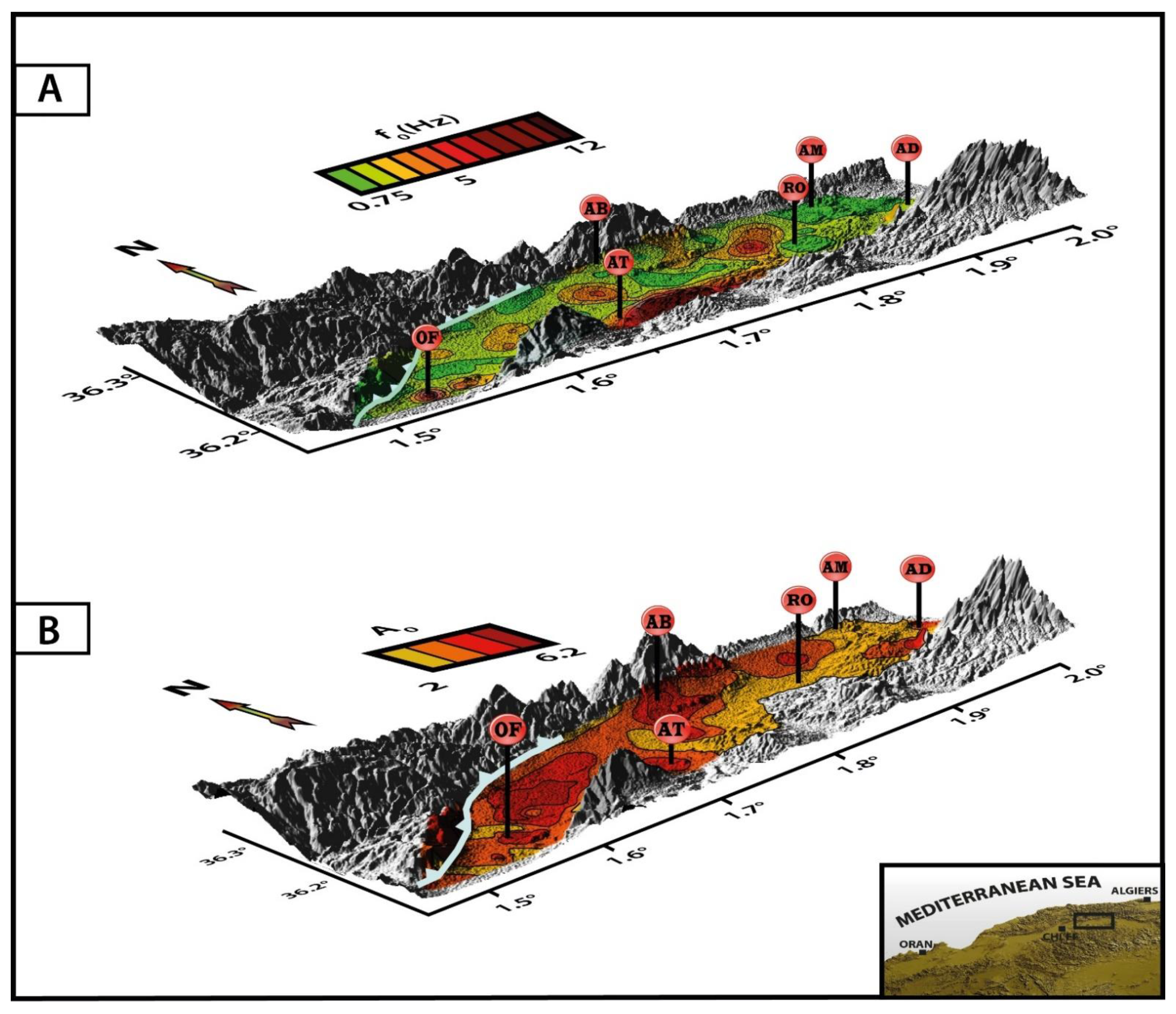
The resonance frequencies and the corresponding amplitudes obtained from the HVSR analysis are mapped in Figure 9. The frequencies range between 0.75 and 12 Hz, while the amplitudes vary from 2 to 6.2. The obtained HVSR curves contain one frequency peak, two peaks, and multiple peaks. Curves with two frequency peaks are predominant, especially in the Quaternary plain.
In the Oued-Fodda Plain (Zone1), the predominant resonance frequencies of the soil vary between 1.5 and 3 Hz, and the corresponding amplitudes vary between 2 and 6. However, particularly in the center of Oued-Fodda city, higher frequencies, between 5 and 12 Hz, are observed. This high-frequency range is related to the outcropping bedrock in the area [22]. In the village of Zbabdja, about 3 km west of Oued-Fodda city, the frequencies are around 1.5 Hz. In terms of shape, two types of curves are observed in this zone: curves with two frequency peaks are predominant in the Oued-Fodda Plain, while curves with one peak were obtained only from recordings in the central parts of Oued-Fodda city and Zbabdja village. Second peaks at higher frequencies are related to impedance contrasts in the soil column at shallow depths [22]. These peaks are only observed at sites located on Holocene alluviums. This allowed us to deduce that this shallow impedance contrast is responsible for the second frequency peaks that are between the Holocene silt layer and the Pleistocene gravel and conglomerate layers.
In the Sara-El-Maarouf anticline, the predominant resonance frequency is around 2 Hz, while the amplitudes of the peaks range between 2.5 and 4.5. The second peaks at higher frequencies appear to be related to the impedance contrast between the Upper Pliocene sands and the Lower Pliocene sandstones.
In the Carnot Plain (Zone 2), the predominant resonance frequencies vary between 0.75 and 5 Hz. The corresponding amplitudes vary from 2.2 to 5.8. HVSR curves with one frequency peak, two peaks, and multiple peaks were observed in this area.
The variation in shape for these curves is mainly related to the variation in the lithology, the apparition of new sedimentary layers, and the disappearance of others at some places, caused by different factors that affect the sedimentation process as erosions and faults. Concerning the shapes of the peaks, they are mainly controlled by the dipping angles of the different layers [54,57].
Peaks at higher frequencies (between 8 and 12 Hz) are observed on the hills overlooking the El-Attaf city from the southwest. These peaks appear to be caused by the outcropping Cretaceous marls. In the city of El-Abadia, the resonance frequency is around 2 Hz, while in El-Attaf city, it is around 3 Hz.
In the third zone, the resonance frequencies range between 1.3 and 3 Hz. The corresponding amplitudes vary between 2.2 and 3.5. Two types of HVSR curves were obtained: curves with one frequency peak in the southern part, and curves with two frequency peaks in the northern part. The frequency of the second peak varies from 5 to 12 Hz and appears to be related to an impedance contrast between the Holocene and Pleistocene alluviums at shallow depths. In the city of Ain-Defla, the resonance frequency of the soil increases from 1.8 to 3 Hz, from north to south, respectively. The corresponding peak amplitudes are around 5.

6.2. F–K Analysis: Surface Wave Dispersion Curves

In Figure 10, the dispersion curves estimated from the different deployed arrays are shown. In some places, a single array was enough to obtain a reliable dispersion curve, while, in other places, two arrays of different apertures were implemented, obtaining an average dispersion curve. The frequency range is fixed by the theoretical wavenumber limits (Kmin/2, Kmax), which depend on the array configuration and aperture (Figure 8). The curves are, therefore, not very reliable outside the theoretical wavenumber limits.
In the city of Oued-Fodda and its surroundings, the analysis of the array measurements at sites AR1, AR2, AR3, AR4, and AR5 provided dispersion curves between 2.5 and 10 Hz. The dispersion curves obtained from the array recording AR6 in the city of El-Attaf are reliable in the frequency range between 5 and 10 Hz, and between 2.5 and 8 Hz in the city of El-Amra (AR7).

6.3. Electrical Resistivity Tomography

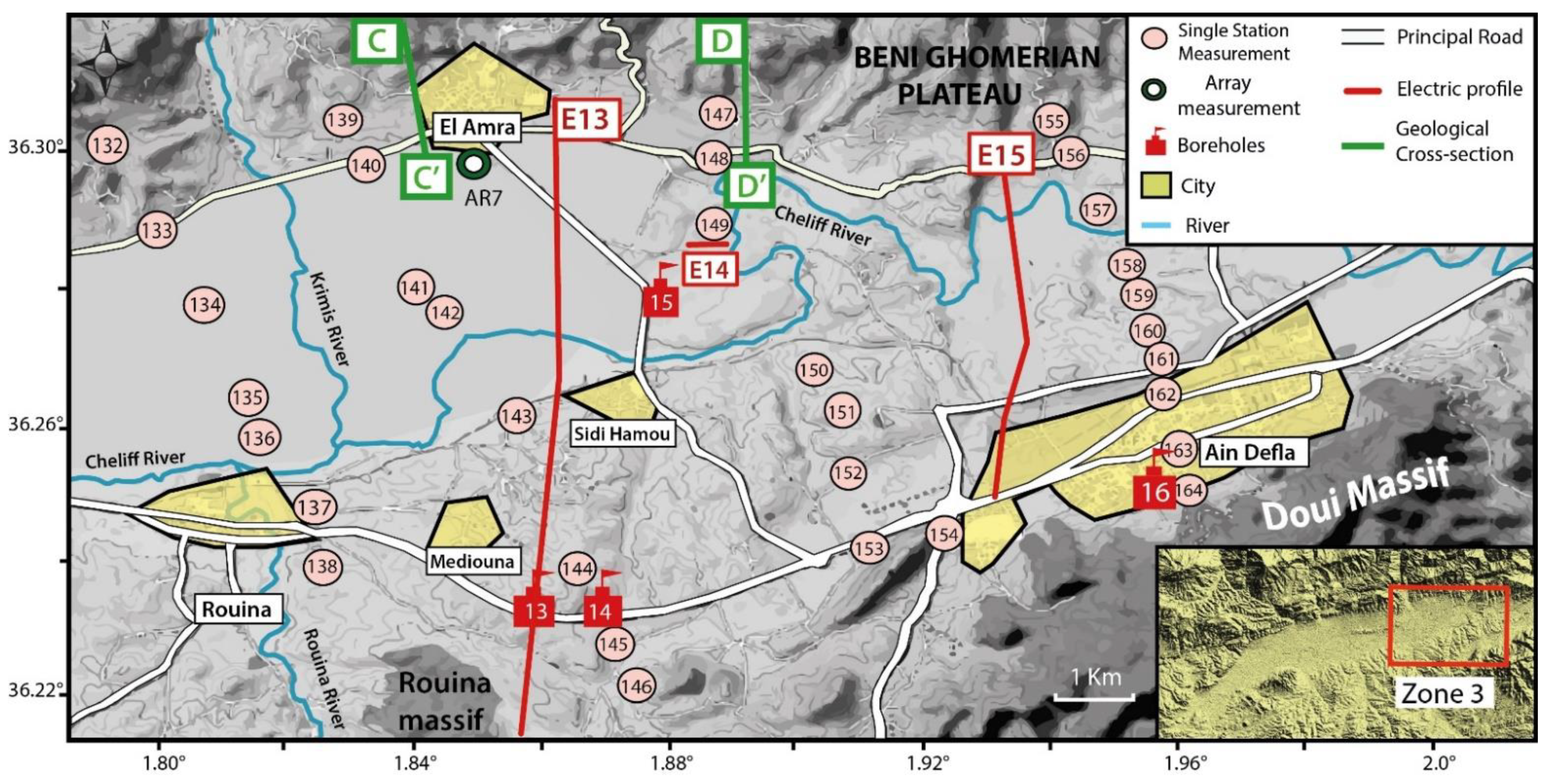
The electrical resistivities, obtained from measurements in Mechta-Nouasser (E1, Figure 5) and in the southeast of El-Amra (E14, Figure 6), are shown in Figure 11. In order to interpret the obtained results, we used the resistivity scale established by the CGG [7] for the Middle-Chelif Basin (left panel in Figure 11).
For the resistivity profile (E1), the depth of the investigation of 115 m allowed for the identification of the two Quaternary layers. The thicknesses of these two layers (1 and 2 in Figure 11) appeared to be about 50 m (~10 m of Holocene and ~40 m of Pleistocene alluviums). For the profile (E14), the depth of investigation was 105 m. The resistivity scale for the Middle-Chelif Basin allowed us to identify four different sedimentary layers; the two top layers belong to the Quaternary, while the underlying layers are attributed to the Miocene. The thickness of the Quaternary deposits is about 35 m (~10 m of Holocene and ~25 m of Pleistocene).
The results of the electrical resistivity measurements in Mecheta-Nouasser (E1) and El-Amra (E14) allowed us to fix the thicknesses of the Quaternary layers (Holocene and Pleistocene) for the inversion of the HVSR curves recorded at Sites 77, 78, and 149.

6.4. Shear-Wave 2D Velocity Profiles

The inversion of the obtained HVSR curves allowed for the retrieval of the S-wave velocity models at each site. For sites where array measurements were also taken, the joint inversion of the obtained dispersion and HVSR curves was carried out. The number of analyzed layers, as well as the range of the respective Vs and thickness parameters, have been constrained according to previous information obtained from geological cross-sections, boreholes, and geotechnical studies (see Table 1). The aim was to obtain a result closer to the true model by minimizing the misfit value. Some examples are shown in Figure 12.
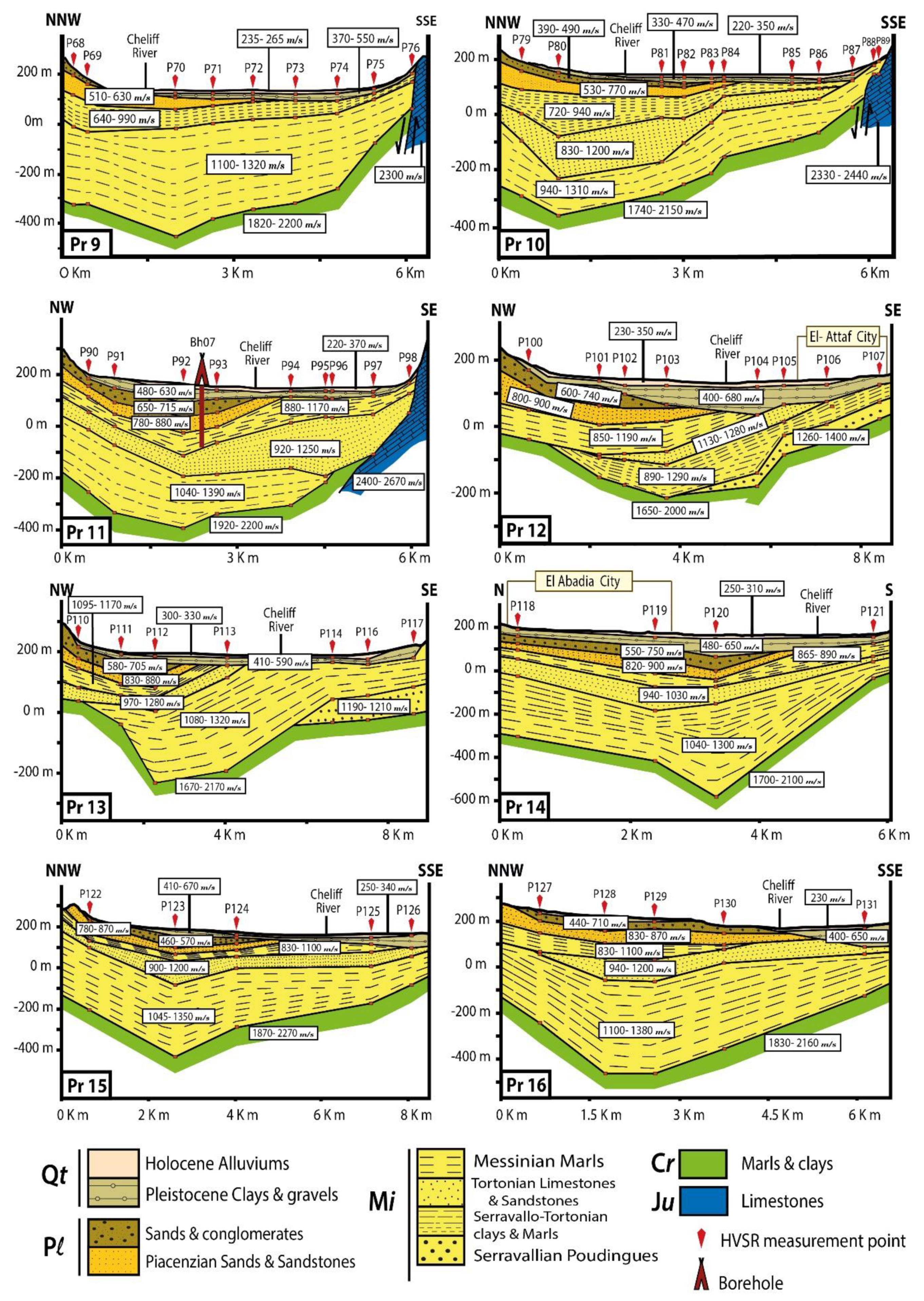
For the first zone, the eight obtained 2D velocity profiles are mapped in Figure 13. The two uppermost layers in the plain correspond to the two Quaternary stages, the Holocene and Pleistocene, mainly composed of alluviums. The obtained Vs values for the Holocene alluviums vary between 210 and 350 m/s. This range is explained by the lateral variation between clays and silts. For the Pleistocene layer, the Vs value ranges between 405 and 630 m/s. This variation is due to the alternance between grave and clay facies. The high contrast in velocity between the two Quaternary stages is responsible for the second frequency peak in the area. The thickness of the Holocene formation does not exceed 10 m, while the Pleistocene deposits reach a maximum thickness of 65 m north of Oued-Fodda city.
On the Sara-El-Maarouf anticline, in the profiles Pr6, Pr7, and Pr8 (Figure 13), the two topmost layers correspond to the Upper and Lower Pliocene. The Vs values obtained for the Upper Pliocene sands vary between 300 and 400 m/s, and between 610 and 780 m/s for the Lower Pliocene sandstones. As for the Quaternary stages down in the plain, the contrast in velocity between the two Pliocene layers is responsible for the second frequency peak in the HVSR curves obtained from recordings on the Sara-El-Maarouf anticline. These formations reach a maximum thickness of 100 m in the oriental part of the anticline. A thin Tortonian limestone layer lies under the Pliocene layers, for which the Vs value ranges between 650 and 900 m/s. This layer dips into the northwest and is not present in the Oued-Fodda Plain. The Quaternary layers in the plain are, therefore, lying directly over a thick layer composed of Serravallo-Tortonian marls and clays. This is the thickest sedimentary layer in the Middle-Chelif Basin. It reaches a maximum thickness of 250 m in this zone. The Vs value for this layer varies between 850 and 1290 m/s. This formation is in direct contact with the Cretaceous bedrock, which is mainly composed of hard marls. The obtained shear-wave velocity of these marls varies between 1700 and 2300 m/s in this zone.
In the profiles, Pr 6, Pr 7, and Pr 8 (Figure 13), we can see that the sediments of the plain are separated from the ones of the Sara-El-Maarouf anticline by a deep reverse fault that outcrops at the surface, the so-called "El-Asnam fault". The surface trace coordinates of the fault, along with its dipping angle calculated in Yielding [8] and Ouyed [11], were taken into consideration for the inversion process. In the profile, Pr 7, we can observe normal faults at the top of the anticline. The surface trace of these faults was observed during the HVSR measurement campaign. The important variations in the thickness of the layers between the measurement points, P54, P55, P56, and P57 (Profile Pr7 in Figure 12), allowed us to obtain an approximate idea on the fault position under the surface. The presence of normal faults at the top of the Sara-El-Maarouf anticline was highlighted before by Philip and Meghraoui [19]. This normal faulting comes as a result of the extension of the surface layers of the anticline due to the vertical slip on the El-Asnam fault [11,19].
The eight 2D velocity profiles in the Carnot Plain are mapped in Figure 14. Unlike the first zone, the synclinal shape of the basin is clearly visible in this zone. The depocenters are located north of the Chelif River, as attested by the CGG study [7]. The highest depths of the basin are observed around the city of El-Abadia, with a maximum depth of 760 m (P120 in Profile Pr14, Figure 14). Compared to the first zone, the lithostratigraphic column contains two additional layers of the Miocene age; the Messinian marls and the Serravallian poudingues. The Holocene alluviums have a Vs value between 220 and 370 m/s and reach a maximum thickness of 21 m in the middle of the plain. The Pleistocene alluviums reach a maximum thickness of 86 m, and the Vs value for this layer varies between 330 and 680 m/s. The Upper and Lower Pliocene layers that outcrop on a narrow band north of the plain, dip south under the Quaternary layers and disappear in the middle of the plain. The absence of Pliocene deposits in the south is due to marine regression during the late-Miocene early-Pliocene period, where the shorelines were located in the middle of the plain [2]. These formations are therefore thicker in the north and reach thicknesses of 145 m (P92 in Profile Pr11, Figure 14). The Vs value for the Upper Pliocene sands and conglomerates varies between 390 and 750 m/s, and between 510 and 900 m/s for the Lower Pliocene sandstones. The Pliocene deposits lie over the Messinian blue marls, the uppermost layer of the Miocene. The Miocene deposits occupy most of the sedimentary column of the Middle-Chelif Basin, reaching thicknesses of 550 m. However, there is no impedance contrast between the four Miocene layers in the area. The Vs values for the blue marls stands between 640 and 1190 m/s. For the Tortonian sandstones, they vary between 830 and 1280 m/s, and between 890 and 1380 m/s for the Serravallo-Tortonian clays and marls. For the Serravallian poudingues and conglomerates, the shear-wave velocities vary between 1190 and 1400 m/s.
For the Cretaceous bedrock, the Vs varies between 1650 and 2270 m/s. This variation is due to the lateral change of formations from Senonian clays and marls to Albian marls and limestones. In the southwestern part of the plain (Profiles Pr 9, Pr 10, and Pr 11, Figure 14), the Jurassic limestones that compose the Temoulga Massif dip vertically under the Neogene sediments, with a faulted contact between the limestones and the Cretaceous marls [35]. The calculated shear-wave velocities for the Jurassic limestones vary between 2300 and 2670 m/s.
The third zone, which covers the Rouina-Ain-Defla region, has a different local geological context. The vast Quaternary plain gives way to hills and plateaus. The four 2D velocity profiles realized for this zone are mapped in Figure 15. The lithostratigraphic column is dominated by the Tortonian sandstones and Serravallo-Tortonian clays and marls. The Vs values for sediments are in the same range as for the second zone. In the profile, Pr20 (Figure 15), we can see all the structural complexity that exists in this zone of closure.
The sedimentary layers become thinner and lie over different types of bedrock. The old formations become more rugged to the south because of the presence of the epimetamorphic Doui Massif (Figure 2). North of the city of Ain-Defla (Profile Pr 20), the Albian clays and marls are separated from the Jurassic limestones by a block of Neocomian schists, which belongs to the Arib Massif that overlooks the Upper-Chelif Plain. The presence of the Neocomian schists marks the transition between the Middle and Upper Chelif Basin. The Vs values for this formation vary between 2280 and 2410 m/s.
The average Vp/Vs ratio was calculated from the 164 velocity models. The averaged ratio for the sedimentary column is 1.95. For the bedrock formations, the averaged ratio is 1.76. This value is in agreement with the 1.7 found by Bellalem [53] in a seismic tomography study.
The depths to seismic bedrock are mapped in Figure 16. We can see that the basin reaches higher depths in a narrow band stretching from the west of El-Abadia to El-Amra, and reaches a maximum depth of 760 m (P120 in Profile Pr14, Figure 14), which is very close to the 800 m measured by the CGG [7].

7. Conclusions

In the present work, ambient vibration data were used to investigate the soil characteristics and the site effects in the Middle-Chelif Basin, with both single-station and array measurements. The region is home to over 400,000 inhabitants, distributed over its six main cities: Ain-Defla, El-Amra, Rouina, El-Abadia, El-Attaf, and Oued-Fodda. Being located on a zone with moderate to high seismic activity, these cities have suffered important building damages during past earthquakes. The fact that most of them are built on soft sediment layers has played a role in amplifying the ground shaking and the lengthening of its duration.
The first tens of meters of the topsoil column play an important role in ground shaking amplification during an earthquake. In our case study, it corresponds principally to the thickness of the Quaternary layers. In the major part of the basin, these layers lie directly over the Miocene sediments, which creates an important impedance contrast. Thus, the thickness of the Quaternary layers and the corresponding Vs values had to be determined with more precision. For this purpose, seismic noise array measurements and electrical resistivity measurements were carried out. The HVSR technique was applied on ambient vibration recordings at 164 sites, and F–K analysis was applied on array recordings at 7 sites. The obtained HVSR curves allowed us to identify the soil resonance frequencies at each site. The F–K analysis allowed us to retrieve the surface wave dispersion curve at each of the 7 sites. The HVSR and dispersion curves were then jointly inverted to obtain the Vs profiles at each site.
The analysis of the HVSR curves showed the existence of different types of curves: curves with one, two, and multiple frequency peaks. The HVSR curves with two peaks are predominant in the Middle-Chelif Plain. The predominant soil resonance frequencies vary between 0.75 and 12 Hz. This wide range of frequencies is explained by the synclinal aspect of the basin, as well as the thinning of the sedimentary layers on its edges. The corresponding amplitudes vary between 2 and 6.2. However, the amplitudes obtained from the HVSR analysis may not be a reliable estimation of true amplification. The high-frequency peaks (between 5.9 and 12 Hz) appear to be related to an impedance contrast between the Holocene and Pleistocene alluviums at shallow depths.
In the Middle-Chelif Plain, the topmost layer is composed of thin Holocene alluvial deposits, for which the shear-velocity (Vs) ranges between 210 and 370 m/s. The largest thickness observed for this layer is 21 m. For the Pleistocene deposits, the Vs value varies between 330 and 680 m/s, with a maximum observed thickness of 86 m. The Pliocene deposits are present only in the northern part of the plain and on the Sara-El-Maarouf anticline in the west. The shear-wave velocity varies between 300 and 750 m/s for the Upper Pliocene sands and conglomerates, and between 510 and 900 m/s for the Lower Pliocene sandstones. The largest observed thickness for the Pliocene layers is 145 m, while the Miocene deposits occupy a major part of the sedimentary column, often composed of four distinct layers. Their thickness reaches 550 m around the city of El-Abadia. From the Messinian stiff marly formations to the Serravallian poudingues, the Vs values vary from 640 to 1450 m/s.
In the southern part of the Middle-Chelif Plain, Jurassic formations outcrop in succession on the massifs of Doui, Rouina, and Temoulga. The Jurassic limestones are dipping, generally north, and constitute the bedrock for the Neogene deposits in this part of the basin. The shear-wave velocity for these formations varies between 2300 and 2670 m/s. However, in a major part of the basin, the sedimentary deposits lie over a Cretaceous bedrock, for which the Vs values range between 1620 and 2300 m/s. The calculated Vp/Vs ratio for the sedimentary column is 1.95. For the bedrock formations, the ratio is 1.76.
The obtained velocity and resistivity profiles highlight the existence of important lateral variations in the velocity and resistivity of the whole sedimentary column. This variation is directly linked with variations in lithology (lateral change of facies), caused by different factors that have affected the sedimentation process in the Middle-Chelif Basin (marine regression and transgression episodes during the Miocene and Pliocene, erosions, faults, etc.).
The sedimentary layers show a synclinal aspect in the plain of Carnot, unlike the Oued-Fodda and Ain-Defla regions, where the underground structures are rugged, affected by different faults, folds, and outcrops. The depocenters in the Middle-Chelif Basin appear to be located in a narrow band extending from the western part of the town of El-Abadia to the northern part of the town of Rouina. The maximum observed depth to bedrock is 760 m.
The thickness of the sedimentary layers is different beneath the cities situated in the northern and southern parts of the Middle-Chelif Plain. In the city of Ain-Defla, which backs onto the northern flank of the epimetamorphic Doui Massif, the sedimentary column does not exceed 60 m. While in the cities of Oued-Fodda and El-Attaf, which were built around the western and eastern parts of the Temoulga Massif, respectively, the sedimentary column reaches a thickness of 200 m. However, the cities of Rouina, El-Abadia, and El-Amra are lying over a thick sedimentary cover that exceeds 300 m.
The cities cited in this study extend over a region where strong earthquakes with secondary effects (liquefaction, landslides, etc.) have already occurred several times before. Therefore, this study would like to be a contribution to a better assessment of the seismic hazard in the Chelif-Basin. The results obtained in this study can be used, for example, in the modeling of strong ground motions in order to update the Algerian seismic code.

Author Contributions

A.I. acquired and processed the data and wrote the paper. F.S. proposed the methodology and reviewed the paper. A.Y.-C. reviewed and supervised the paper. J.J.G.-M. helped with array processing and reviewed the paper. A.M. performed the electrical prospecting. All authors have read and agreed to the published version of the manuscript.

Funding

This study was funded by the Consellería de Participación, Transparencia, Cooperación y Calidad Democrática de la Generalitat Valenciana, and by Research Group VIGROB-116 (University of Alicante).

Institutional Review Board Statement

Not applicable.

Informed Consent Statement

Not applicable.

Data Availability Statement

The data presented in this study are available upon request from the corresponding author. The data are not publicly available because of their large size.

Acknowledgments

We would like to thank Hamai Lamine for providing the equipment for the resistivity measurements. We also thank Z.Sahari for her help with the lithological cross-sections. A special thanks to the CRAAG team that participated in field measurements: A. Belahouene, A. Sebbane, A. Saadi, B. Melouk, O. Haddad, and R. Chimouni.

Conflicts of Interest

The authors declare no conflict of interest.

References

  1. Meghraoui, M. Géologie des Zones Sismiques du Nord de l’Algérie: Paléosismologie, Tectonique Active et Synthèse Sismotectonique. Ph.D. Thesis, University of Paris-Sud, Paris, France, 1988. [Google Scholar]
  2. Perrodon, A. Etude géologique des bassins sublittoraux de l’Algérie occidentale. Publ. Serv. Carte Géol. l’Algérie. NS Bull. 1957, 12, 328. [Google Scholar]
  3. Thomas, G. Géodynamique d’un Bassin Intramontagneux: Le Bassin du Bas Chéliff Occidental (Algérie) Durant le Mio-Plio-Quaternaire. Ph.D. Thesis, University of Pau, Pau, France, 1985. [Google Scholar]
  4. Yelles-Chaouche, A.; Boudiaf, A.; Djellit, H.; Bracene, R. La tectonique active de la région nord-algérienne. Comptes Rendus Geosci. 2006, 338, 126–139. [Google Scholar] [CrossRef]
  5. Serpelloni, E.; Vannucci, G.; Pondrelli, S.; Argnani, A.; Casula, G.; Anzidei, M.; Baldi, P.; Gasperini, P. Kinematics of the western Africa Eurasia plate boundary from focal mechanisms and GPS data. Geophys. J. Int. 2007, 169, 1180–1200. [Google Scholar] [CrossRef]
  6. Agence Nationale des Ressources Hydroliques (ANRH). Assessment of the Water Resources of the Middle Cheliff Alluvial Aquifer; Agence Nationale des Ressources Hydroliques: Bir Mourad Raïs, Algeria, 2006. [Google Scholar]
  7. Compagnie Generale de Geophysique (CGG). Geophysical Study of the Cheliff Plain. Internal Report; Compagnie Generale de Geophysique: Alger, Algeria, 1969. [Google Scholar]
  8. Yielding, G.; Jackson, J.A.; King, G.C.P.; Sinvhal, H.; Vita-Finzi, C.; Wood, R.M. Relations between surface deformation, fault geometry, seismicity and rupture characteristics during the El Asnam (Algeria) earthquake of 10 October 1980. Earth Planet Sci. Lett. 1981, 56, 287–304. [Google Scholar] [CrossRef]
  9. Meghraoui, M. Etude Neotectonique de la Region Nord-Est d’El ASNAM: Relation Avec le Seisme du 10.10. 1980. Ph.D. Thesis, University of Paris, Paris, France, 1982. [Google Scholar]
  10. Mokrane, A.; Ait Messaoud, A.; Sebai, A.; Ayadi, A.; Bezzeghoud, M. Les Séismes en Algérie de 1365 à 1992; Centre de Recherche en Astronomie Astrophysique et Géophysique (CRAAG): Algiers, Algeria, 1994. [Google Scholar]
  11. Ouyed, M. Le Tremblement de Terre d’El Asnam du 10 Octobre 1980: Étude des Répliques. Algérie. Ph.D. Thesis, Grenoble Alpes University, Grenoble, France, 1981. [Google Scholar]
  12. Delgado, J.; Lopez-casado, C.; Estevez, A.; Giner, J.; Cuenca, A.; Molina, S. Mapping soft soils in the Segura river valley (SE Spain): A case study of microtremors as anexploration tool. J. Appl. Geophys. 2000, 45, 19–32. [Google Scholar] [CrossRef]
  13. Garcia-Jerez, A.; Luzon, F.; Navarro, M.; Perez-Ruiz, J.A. Characterization of the sedimentary cover of the Zafarraya Basin, Southern Spain, by means of ambient noise. Bull. Seismol. Soc. Am. 2006, 96, 957–967. [Google Scholar] [CrossRef]
  14. Luzon, F.; Al-Yuncha, Z.; Sanchez-Sesma, F. A Numerical Experiment on the Horizontal to Vertical Spectral Ratio in Flat Sedimentary Basins. Pure Appl. Geophys. 2001, 158, 2451–2461. [Google Scholar] [CrossRef]
  15. Mundepi, A.; Galiana-Merino, J.; Asthana, A.L.; Rosa-Cintas, S. Soil characteristics in Doon Valley (north west Himalaya, India) by inversion of H/V spectral ratios from ambient noise measurements. Soil Dyn. Earthq. Eng. 2015, 77, 309–320. [Google Scholar] [CrossRef]
  16. Rosa-Cintas, S.; Galiana-Merino, J.J.; Molina, S.; Rosa-Herranz, J.; García-Fernández, M.; Jiménez, M. Soil characterization in urban areas of the Bajo Segura Basin (Southeast Spain) using H/V, F–K and ESAC methods. J. Appl. Geophys. 2011, 75, 543–557. [Google Scholar] [CrossRef]
  17. Talaganov, K.; Aleksovski, D.; Milutinovic, Z.; Ameur, B.; Arsovski, M.; Jancevski, J.; Andreevski, V. Studies for Elaboration of the Code for Repair and Strengthening of Damaged Buildings in the Region of El Asnam: Engineering Geology, Geotechnical and Geophysical Characteristics of the Town of El Asnam and Other Sites; IZIIS Report; Institute of Earthquake Engineering and Engineering Seismology (IZIIS): Skopje, North Macedonia, 1982; p. 82-55. [Google Scholar]
  18. Woodward-Clyde-Consultants. Seismic Microzonation of Ech-Chellif Region, Algeria; Woodward-Clyde-Consultants: Blue Bell, PA, USA, 1984. [Google Scholar]
  19. Philip, H.; Meghraoui, M. Structural analysis and interpretation of the surface deformations of the El Asnam earthquake of 10 October 1980. Tectonics 1983, 2, 17–49. [Google Scholar] [CrossRef]
  20. Layadi, K.; Semmane, F.; Yelles-Chaouche, A. S-wave velocity structure of Chlef City, Algeria, by inversion of Rayleigh wave ellipticity. Near Surf. Geophys. 2018, 16, 328–339. [Google Scholar] [CrossRef]
  21. Layadi, K.; Semmane, F.; Yelles-Chaouche, A. Site-Effects Investigation in the City of Chlef (Formerly El-Asnam), Algeria, Using Earthquake and Ambient Vibration Data. Bull. Seismol. Soc. Am. 2016, 106, 2185–2196. [Google Scholar] [CrossRef]
  22. Issaadi, A.; Semmane, F.; Yelles-Chaouche, A.; Galiana-Merino, J.; Layadi, K. A Shear-Wave Velocity Model in the City of Oued-Fodda (Northern Algeria) from Rayleigh Wave Ellipticity Inversion. Appl. Sci. 2020, 10, 1717. [Google Scholar] [CrossRef] [Green Version]
  23. Bouchelouh, A.; Bensalem, R.; Zaourar, N.; Machane, D.; Moulouel, H.; Oubaiche, E.H. The Miocene Roof Mapping Using Microtremor Recording and Electrical Survey Method in Blida City, Algeria. Pure Appl. Geophys. 2017, 175, 287–301. [Google Scholar] [CrossRef]
  24. Tebbouche, M.; Machane, D.; Chabane, S.; Oubaiche, E.H.; Meziani, A.; Ait Benamar, D.; Moulouel, H.; Cheikh Lounis, G.; Bensalem, R.; Bendaoud, A. Imagery of the metamorphic bedrock roof of the Sahel active fault in the Sablettes (Algiers) reclaimed area by ambient vibration HVSR. Arab. J. Geosci. 2017, 10, 292. [Google Scholar] [CrossRef]
  25. Nakamura, Y. A method for dynamic characteristics estimation of subsurface using microtremor on the ground surface. Railw. Tech. Res. Inst. Q. Rep. 1989, 30, 25–33. [Google Scholar]
  26. Nogoshi, M.; Igarashi, T. On the amplitude characteristics of ambient noise (Part 2). J. Seismol. Soc. Jpn. 1971, 24, 26–40. [Google Scholar]
  27. Capon, J. High-resolution frequency-wavenumber spectral analysis. Proc. IEEE 1969, 57, 1408–1419. [Google Scholar] [CrossRef] [Green Version]
  28. Capon, J.; Greenfield, R.; Kolker, R. Multidimensional maximum-likelihood processing of a large aperture seismic array. Proc. IEEE 1967, 55, 192–211. [Google Scholar] [CrossRef]
  29. Kelly, E.J.; Levin, M.J. Signal Parameter Estimation for Seismometer Arrays; Massachusetts Institute of Technologies, Lincoln Lab: Lexington, MA, USA, 1964. [Google Scholar]
  30. Lacoss, R.T.; Kelly, E.J.; Toksoz, M.N. Estimation of seismic noise structure using Array. Geophysics 1969, 29, 21–38. [Google Scholar] [CrossRef]
  31. Delteil, J. Tectonique de la Chaîne Alpine en Algérie D’après L’étude du Tel Oranais Oriental. Monts de la Mina, Beni Choughrane, Dahra. Ph.D. Thesis, University of Nice, Nice, France, 1974; 294p. [Google Scholar]
  32. Brives, A. Les Terrains Miocènes du Bassin du Chélif et du Dahra; Imprimerie, P., Ed.; Fontana & Cie: Alger, Algérie, 1897. [Google Scholar]
  33. Mattauer, M. Etude Géologique de l’Ouarsenis Oriental; Publication du Service de Cartographie d’Algérie, n°17; Service de Cartographie d’Algérie: Alger, Algeria, 1958. [Google Scholar]
  34. Kireche, O. Etude Géologique et Structurale des Massifs de la Plaine du Chéliff (Doui, Rouina, Temoulga). Ph.D. Thesis, University of Algiers, Algiers, Algeria, 1977. [Google Scholar]
  35. Repal, S.N. Le Basin Néogène du Chélif. In Proceedings of the XIXe Congrés de Géologie International, Service Geologique de l’Algérie, Algiers, Algeria, 8–15 September 1952; p. 56. [Google Scholar]
  36. Brives, A.; Jackob, M.; Ficheur, M. Carte Géologique De Oued-Fodda 1/50,000; Service Géologique de l’Algérie: Algiers, Algeria, 1906. [Google Scholar]
  37. Field, E.H.; Jackob, K.H. A comparison and test of various site response estimation techniques, including three that are non reference—Site dependent. Bull. Seismol. Soc. Am. 1995, 85, 1127–1143. [Google Scholar]
  38. Arai, H.; Tokimasu, K. S-wave velocity profiling by inversion of microtremor H/V spectrum. Bull. Seismol. Soc. Am. 2004, 94, 53–63. [Google Scholar] [CrossRef]
  39. Bonnefoy-Claudet, S.; Cornou, C.; Bard, P.Y.; Cotton, F.; Moczo, P.; Kristek, J.; Fäh, D. H/V ratio: A tool for site effects evaluation: Results from 1D noise simulations. J. Appl. Geophys. 2006, 167, 827–837. [Google Scholar] [CrossRef] [Green Version]
  40. Lachet, C.; Bard, P.Y. Numerical and theoretical investigations on the possibilities and limitations of Nakamura’s technique. J. Phys. Earth 1994, 42, 377–397. [Google Scholar] [CrossRef]
  41. Rosa-Cintas, S.; Galiana-Merino, J.; Rosa-Herranz, J.; Molina, S.; Martínez-Esplá, J. Polarization analysis in the stationary wavelet packet domain: Application to HVSR method. Soil Dyn. Earthq. Eng. 2012, 42, 246–254. [Google Scholar] [CrossRef]
  42. La Rocca, M.; Chiappetta, G.; Gervasi, A.; Festa, R.L. Non-Stability of the noise HVSR at sites near or on topographic heights. Geophys. J. Int. 2020, 222, 2162–2171. [Google Scholar] [CrossRef]
  43. Bonnefoy-Claudet, S.; Kohler, A.; Cornou, C.; Wathelet, M.; Bard, P.Y. Effects of Love waves on microtremor H/V ratio. Bull. Seismol. Soc. Am. 2008, 98, 288–300. [Google Scholar] [CrossRef]
  44. Wathelet, M. An improved neighborhood algorithm: Parameter conditions and dynamic scaling. Geophys. Res. Lett. 2008, 35, L09301. [Google Scholar] [CrossRef] [Green Version]
  45. Wathelet, M.; Jongmans, D.; Ohrnberger, M. Surface-wave inversion using a direct search algorithm and its application to ambient vibration measurements. Near Surf. Geophys. 2004, 2, 211–221. [Google Scholar] [CrossRef] [Green Version]
  46. Maresca, R.; Galluzzo, D.; Del-Pezzo, E. H/v spectral ratios and array techniques applied to ambient noise recorded in the Colfiorito Basin, Central Italy. Bull. Seismol. Soc. Am. 2006, 96, 490–505. [Google Scholar] [CrossRef]
  47. Rost, S.; Thomas, C. Array Seismology: Methods and Applications. Rev. Geophys. 2002, 40, 1008. [Google Scholar] [CrossRef] [Green Version]
  48. Levin, M.J. Maximum-Likelihood Array Processing, Seismic Discrimination Semiannual Technical Summary; Lincoln Laboratory, Massachusetts Institute of Technology: Lexington, MA, USA, 1964. [Google Scholar]
  49. Allaud, L.; Martin, M. Schlumberger, History of a Technique; John Wiley & Sons: New York, NY, USA, 1977. [Google Scholar]
  50. Loke, M.H.; Barker, R.D. Practical techniques for 3Dresistivity surveys and data inversion techniques. Geophys. Prospect. 1996, 44, 499–524. [Google Scholar] [CrossRef]
  51. Schlumberger, C.; Schlumberger, M.; Doll, H.G. Electrical Coring: A Method of Determining Bottom-Hole Data by Electrical Measurements. In Transactions of the American Institute of Mining and Metallurgical Engineers; Paper 462; American Institute of Mining, Metallurgical, and Petroleum Engineers: New York, NY, USA, 1932; Volume 100. [Google Scholar]
  52. Dahlin, T.; Loke, M.H. Resolution of 2D Wenner resistivity imaging as assessed by numerical modelling. J. Appl. Geophys. 1998, 38, 237–249. [Google Scholar] [CrossRef] [Green Version]
  53. Bellalem, F.; Bounif, M.; Koulakov, I. P and S waves tomographic analysis of the area of El Asnam’s 1980 ms 7.3 earthquake (Algeria) from its aftershock sequence. J. Seismol. 2015, 19, 253–264. [Google Scholar] [CrossRef]
  54. Acerra, C.; Aguacil, G.; Anastasiadis, A.; Atakan, K.; Azzara, R.; Bard, P.-Y.; Basili, R.; Bertrand, E.; Bettig, B.; Blarel, F. Guidelines for the Implementation of the H/V Spectral Ratio Technique on Ambient Vibrations Measurements, Processing and Interpretation; European Commission–EVG1-CT-2000-00026 SESAME; European Commission: Brussels, Belgium, 2004. [Google Scholar]
  55. Soler-Llorens, J.L.; Galiana-Merino, J.; Benabdeloued, N.; Rosa-Cintas, S.; Ortiz-Zamora, J.; Giner-Caturla, J.J. Design and implementation of an Arduino-based plug-and-play acquisition system for seismic noise measurements. Electronics 2019, 8, 1035. [Google Scholar] [CrossRef] [Green Version]
  56. Konno, K.; Ohmachi, T. Ground-motion characteristics estimated from spectral ratio between horizontal and vertical components of microtremor. Bull. Seismol. Soc. Am. 1998, 88, 228–241. [Google Scholar] [CrossRef]
  57. Woolery, E.; Street, R. Quaternary fault reactivation in the fluorspar area fault complex of western Kentucky: Evidence from shallow SH-wave reflection profiles. Seismol. Res. Lett. 2002, 73, 628–639. [Google Scholar] [CrossRef]
Figure 1. Situation of the Middle-Chelif Basin. LCB: Lower-Chelif Basin. MCB: Middle-Chelif Basin. UCB: Upper-Chelif Basin. OF: Oued-Fodda. AB: El-Abadia. AT: El-Attaf. AM: El-Amra. RO: Rouina. AD: Ain-Defla.
Applsci 11 11058 g001
Figure 2. Geological map of the Middle-Chelif Basin. Modified and compiled from [33,36]. The lithological cross-section, AA′, is digitalized from [35]; BB′, CC′, and DD′ are from [32].
Applsci 11 11058 g002
Figure 3. Zonation map of the study area. Red dots correspond to single-station measurements. Red polygons correspond to the limits of the different cities.
Applsci 11 11058 g003
Figure 4. Compiled data in Zone 1.
Applsci 11 11058 g004
Figure 5. Compiled data in Zone 2.
Applsci 11 11058 g005
Figure 6. Compiled data in Zone 3.
Applsci 11 11058 g006
Figure 7. Some examples of the calculated HVSR curves at each zone.
Applsci 11 11058 g007
Figure 8. Theoretical wavenumbers obtained at each array recording site.
Applsci 11 11058 g008
Figure 9. (A) Fundamental frequencies obtained from the HVSR analysis. (B) Amplitudes of the HVSR fundamental frequency peaks. Red circles represent the cities. The blue line represents the surface trace of the El-Asnam fault. OF: Oued-Fodda. AB: El-Abadia. AT: El-Attaf. RO: Rouina. AM: El-Amra. AD: Ain-Defla.
Applsci 11 11058 g009
Figure 10. Surface wave dispersion curves.
Applsci 11 11058 g010
Figure 11. Resistivity profiles. The shear-wave velocity models correspond to the HVSR points, P77 and P78. The top left panel represents the resistivity scale for the Middle-Chelif Basin [7]. The bottom left panel represents the lithological units identified in the resistivity profiles.
Applsci 11 11058 g011
Figure 12. Examples of the inversion results. For each site, the left panels for each site represent the Vs models. The black line corresponds to the best fit model, the dark grey represents models with minimum misfit + 10%. All the tested models are in light grey. In the right panels, we show the computed fundamental mode of the Rayleigh wave ellipticity curve (dark grey curve), and the inverted part of the HVSR curve (black dotted curve). For sites AR1 and AR3, the bottom of the right panel represents the surface wave dispersion curve.
Applsci 11 11058 g012
Figure 13. 2D Shear-wave velocity profiles for Zone 1. Qt: Quaternary. Pl: Pliocene. Mi: Miocene. Cr: Cretaceous.
Applsci 11 11058 g013
Figure 14. Shear-wave velocity profiles for Zone 2. Qt: Quaternary. Pl: Pliocene. Mi: Miocene. Cr: Cretaceous. Ju: Jurassic.
Applsci 11 11058 g014
Figure 15. Shear-wave velocity profiles for Zone 3. Qt: Quaternary. Pl: Pliocene. Mi: Miocene. Cr: Cretaceous. Ju: Jurassic.
Applsci 11 11058 g015
Figure 16. Bedrock depths of the Middle-Chelif Basin. Red circles represent the cities. OF: Oued-Fodda. AB: El-Abadia. AT: El-Attaf. RO: Rouina. AM: El-Amra. AD: Ain-Defla.
Applsci 11 11058 g016
Table 1. Geotechnical information used for the inversion process. Hl: Holocene. Ps: Pleistocene. As: Astian. Pl: Placenzian. Ms: Messinian. Tr: Tortonian. Sr: Seravallian. Sn: Senonian.
Per/Epoch.AgeRockThickness (m)Vp (m/s)Vs (m/s)σ (KN/m3)References
QuaternaryHlAlluviums2–20350–600200–35016–18[6,7,17,18,22]
PsClays &
Conglomerates
10–100600–1700400–70018–22[6,7,17]
PlioceneAsSands &
Conglomerates
10–80550–2000350–75017–22[7,17]
PlSands &
Conglomerates
30–80750–2400500–90019–23[7,17]
MioceneMsMarls30–801100–2900700–120020–24[7,17]
TrLimestones &
Sandstones
40–1501300–3200900–130023–25[7,17]
Sr-TrClays & Marls100–4501200–3400800–140021–25[7,17,35]
SrPoudingues10–601900–36001300–150022–25[35]
CretaceousSnMarls, clays &
Quartzites
-2600–46001800–250024–27[22]
Jurassique-Limestones-3000–50002000–280025–27[53]
Publisher’s Note: MDPI stays neutral with regard to jurisdictional claims in published maps and institutional affiliations.

