Forecasting the Bearing Capacity of the Driven Piles Using Advanced Machine-Learning Techniques

Abstract

Estimating the bearing capacity of piles is an essential point when seeking for safe and economic geotechnical structures. However, the traditional methods employed in this estimation are time-consuming and costly. The current study aims at elaborating a new alternative model for predicting the pile-bearing capacity based on eleven new advanced machine-learning methods in order to overcome these limitations. The modeling phase used a database of 100 samples collected from different countries. Additionally, eight relevant factors were selected in the input layer based on the literature recommendations. The optimal inputs were modeled using the machine-learning methods and their performance was assessed through six performance measures using a K-fold cross-validation approach. The comparative study proved the effectiveness of the DNN model, which displayed a higher performance in predicting the pile-bearing capacity. This elaborated model provided the optimal prediction, i.e., the closest to the experimental values, compared to the other models and formulae proposed by previous studies. Finally, a reliable and easy-to-use graphical interface was generated, namely “BeaCa2021”. This will be very helpful for researchers and civil engineers when estimating the pile-bearing capacity, with the advantage of saving time and money.

1. Introduction

Pile foundations are used to transmit construction loads deep into the ground in order to ensure structure stability [1,2]. Furthermore, computing the bearing capacity of piles is essential when designing economic and safe geotechnical structures [3]. To date, numerous approaches have been conceived for the sake of creating alternative methods and techniques that contain numerical, experimental, and analytical approaches aiming at predicting the bearing capacity of piles [4,5,6]. Among the most frequently used methods is the Cone Penetration Test (CPT), known for producing accurate results in a variety of situations [7,8]. This is probably due to the fact that CPT-based methods have been modeled in harmony with the CPT results, which were proven to estimate more effective different geotechnical properties, and make more precise pile capacity predictions [6]. Other semi-empirical methods have been widely utilized, such as Meyerhof’s formula, which could yield an acceptable pile-bearing capacity [4]. On the other hand, the High-Strain Dynamic Load Test (HSDLT) and the Static Load Test (SLT) have been employed considerably for predicting the pile-bearing capacity [9]. The HSDT is preferable to the SLT, because it operates with a faster, more advanced, and economic technology [2]. This quality supports its paramount importance addressed by the American Standards Test Methods to standardize the HSDT method [1]. The literature on bearing capacity values revealed a relatively close accuracy in both the HSDT and the SLT [1]. Momeni et al. [10] added that HSDT is faster and more economic compared to SLT, but it generally requires several HSDT tests for each project to obtain a reliable result [11]. Hence, increasing the number of HSDT tests is extremely undesirable since it may increase the total project budget. Moreover, other empirical researchers have proposed traditional methods for estimating the bearing capacity [12,13,14,15]. The quality of easiness and common usage has made these methods very important. However, determining the bearing capacity of bored and driven piles by means of the aforementioned methods is found to be time-consuming and costly [16]. This is probably due to the complex behavior of piles, heterogeneity of the soil around piles, material and shape of piles, and their installation. Accordingly, all the proposed methods/models in the literature yielded ineffective predictions [17]. On the other hand, currently, due to emerging new easy-to-use performance software such as PLAXIS, utilizing finite element analysis for which the system is discretized into a number of meshes to obtain axial capacity is of interest [18]. For this reason, numerical methods based on the finite element approach have recently become well-known for the evaluation of bearing capacity, yielding effective results [19,20]. Recently, the application of some new advanced techniques, namely “artificial intelligence (AI)” or “machine learning (ML)”, has witnessed a spectrum of interest, and they provided exceptional results in solving several issues by learning from the available data [21,22].

Subsequently, the use of machine-learning methods to predict pile-bearing capacity has witnessed considerable development since the early 1990s [21,22,23,24]. Several studies are now able to estimate the pile-bearing capacity with a higher degree of precision in comparison to traditional methods. Among the fundamental research dealing with the pile-bearing capacity, Nawari et al. have used one hidden layer of the ANN model by investigating a database consisting of 25 test data. The chosen input parameters included the SPT-N values and geometrical properties. The ANN model efficiently predicted the pile-bearing capacity compared to traditional methods [25]. Furthermore, Mahnesh has predicted the pile-bearing capacity by using Support Vector Machines and Generalized Regression Neural Network with an input layer containing dynamic stress-wave data [26]. He concluded that the Generalized Regression Neural Network was the best model with a high correlation coefficient (0.977). In addition, Milad et al. have developed an effective model based on Artificial Neural Network, genetic programming, and linear regression methods to predict the bearing capacity of piles by learning from 100 samples. They utilized the Flap number, basic properties of the surrounding soil, pile geometry, and pile-soil friction angle as an input layer. The suggested ANN model has better stability compared to the other methods [27]. Jahed et al. used hybrid PSO–ANN to predict the bearing capacity of rock-socketed piles, by taking into consideration soil length to socket length ratio, total length to diameter ratio, uniaxial compressive strength, and standard penetration test. The proposed PSO–ANN model has demonstrated its efficiency since it produced a high correlation coefficient (R = 0.9685) [1]. Moayedi et al. have used ANFIS, GP, and SA–GP for modeling a database consisting of 50 tests. The chosen input parameters included the pile length, pile cross-sectional area, hammer weight, pile set, and drop height. The SA–GP model efficiently predicted the pile-bearing capacity compared to other methods [28]. Shaik et al. have predicted the pile-bearing capacity by using ANFIS and ANFIS–GMDH–PSO with an input layer containing CPT and pile loading test results [29]. They have proven that the metaheuristic hybrid ANFIS–GMDH–PSO model is the best one, with a high correlation coefficient (0.998) [29]. Harandizadeh et al. have used hybrid MLP–GWO and ANFIS–GWO to predict the bearing capacity of piles from the input layer, including pile area, pile length, flap number, average cohesion, and friction angle, average soil-specific weight, and average pile-soil friction angle. The proposed MLP–GWO model has demonstrated that its efficiency yielded a high correlation coefficient (R = 0.991) [30].

Table 1. Proposed machine-learning models in the literature to estimate the pile-bearing capacity.

Authors	Inputs	Methods	Database	References
Nawari et al. (1999)	SPT-N values and geometrical properties	Neural Network	25	[25]
Mahnesh (2011)	Dynamic stress-wave data	Support Vector Machines and Generalized Regression Neural Network	105	[26]
Milad et al. (2015)	Flap number, basic properties of the surrounding soil, pile geometry, and pile-soil friction angle	Artificial Neural Network, Genetic Programming and Linear Regression	100	[27]
Jahed et al. (2017)	Soil length to socket length ratio, total length to diameter ratio, uniaxial compressive strength, and standard penetration test	hybrid PSO–ANN	132	[1]
Moayedi and Jahed (2018)	Internal friction angle of soil located in shaft and tip, pile length, effective vertical stress at pile toe and pile area	ICA-ANN	59	[31]
Yong et al. (2021)	Pile length, pile cross-sectional area, hammer weight, pile set, and drop height	ANFIS, GP, and SA–GP	50	[2]
Shaik et al. (2019)	Internal friction angle of soil located in shaft and tip, effective vertical stress at pile toe, pile area, and pile length	ICA-ANN and ANFIS	59	[29]
Kardani et al. (2020)	Shear resistance angle at the shaft of the pile, soil shear resistance angle at the tip of the pile, length of pile, cross-sectional area of the pile, and effective stress at the tip of the pile	Decision tree, k-nearest neighbor, Multilayer Perceptron Artificial Neural Network, Random Forest, Support Vector Regressor, and Extreme Gradient Boosting	59	[32]
Harandizadeh et al. (2021)	CPT and pile loading test results	ANFIS and ANFIS–GMDH–PSO	72	[30]
Moayedi et al. (2020)	Pile diameter, pile length, relative density, embedment ratio, and both the pile end resistance and base resistance	GA-ANFIS and PSO-ANFIS	20	[28]
Liu et al. (2020)	Laboratory and in situ testing results	ANFIS, ANN, and GA-ANN	43	[33]
Dehghanbanadaki et al. (2021)	Pile area, pile length, flap number, average cohesion and friction angle, average soil-specific weight, and average pile-soil friction angle	MLP–GWO and ANFIS–GWO	100	[34]

summarizes more than ten studies that have used machine-learning models to predict the pile-bearing capacity.

According to the authors’ knowledge, previous studies have been limited mostly to the use of ANN, ANFIS, and SVM methods for predicting the pile-bearing capacity, although recent studies have shown that other techniques could have yielded more effective and accurate results [35,36,37]. Furthermore, they assessed the predictive capability of suggested models depending on only one split to check the data learning validity. Consequently, the ability of their proposed model to overcome over-fitting and under-fitting problems cannot be assured. Moreover, the majority of published papers have proposed machine-learning models in the form of mathematical equations, which are hard to duplicate in future studies. Admittedly, this practice has very little value for other researchers and civil engineers in the field. Conveniently, to overcome these limitations, investigators have presented their optimal models in the form of a programmed interface or a simple script by a well-known programming language such as Python or Matlab for generating the proposed model. This will make it available to anyone interested in the problem of modeling regardless of their proficiency level.

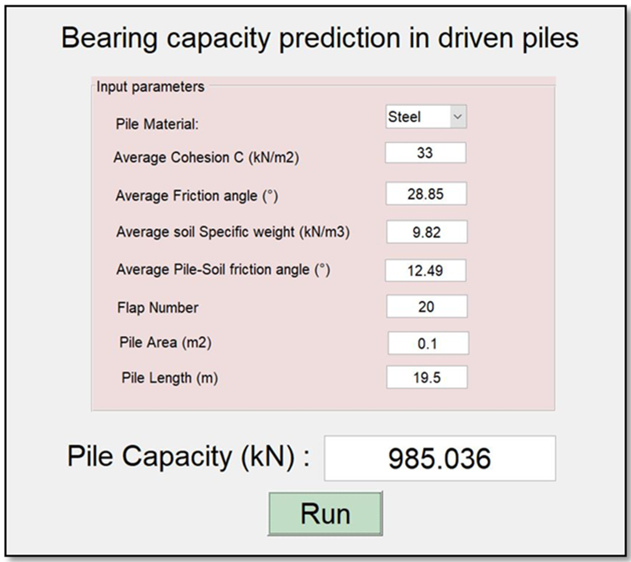
The current study contributes to providing a new alternative model for predicting the pile-bearing capacity based on 12 advanced machine-learning methods, which are applied for the first time for this aim. Furthermore, a high-performance method to estimate the generalization capability of the learning model, and to check the validity of the model for other cases, has been used, namely “K-fold cross-validation analysis”. Finally, in order to treat the hard usage problem of machine-learning models in future studies, the proposed optimal model was used afterwards to develop a GUI public interface. Consequently, the suggested “BeaCa2021” interface is very handy and easy-to-use by civil engineers and researchers, by offering plenty of benefits such as reliability, easiness, and lowering the budget used to predict the pile-bearing capacity from relevant and easily obtained parameters without the need to operate expensive in situ tests.

2. Materials and Methods

2.1. Overview of the Methodology

Several advanced machine learning methods, such as Extreme Deep Neural Network (DNN), Extreme Learning Machine (ELM), Support Vector Regression (SVR), LASSO regression (LASSO), Random Forest (RF), Ridge Regression (Ridge), Partial Least Square Regression (PLSR), Stepwise Regression (Stepwise), Kernel Ridge (KRidge), Genetic Programming (GP), and Least Square Regression (LSR), have been used to learn from 100 samples collected from previous studies [27]. Multiple input parameters, including the pile material, average cohesion (kN/m²), average friction angle (°), average soil-specific weight (kN/m³), average pile-soil friction angle (°), flap number, pile area (m²), and pile length (m), have been used. Firstly, the aforementioned advanced machine-learning methods have been utilized for modeling the input parameters, and their effectiveness was assessed through various statistical indicators. To evaluate the predictive ability of the optimal model, the k-fold cross-validation approach, which is based on five splits, has been employed. Afterward, in order to know which input variables have the biggest effect on the pile-bearing capacity through the proposed model, a sensitivity analysis has been performed via the step-by-step method. Finally, a reliable, easy-to-use, and the graphical interface was designed based on our optimal model in order to help civil engineers and researchers to easily predict the pile-bearing capacity in future studies.

2.2. Database

Choosing the Neural Network inputs is deemed to be the most significant phase for achieving accurate predictions. The selected relevant inputs should cover various aspects of the understudied problem. Besides, several factors have been selected, such as soil characteristics, pile-soil contact characteristics, and geometry and pile characteristics, which can affect the pile-bearing capacity. This study used data from 100 static load-bearing tests on the ultimate bearing capacity (UBC) of both the steel- and the concrete-driven piles from various countries, such as Iran, Mexico, and India [38,39,40,41,42]. The input parameters, including pile material, average cohesion (kN/m²), average friction angle (°), average soil unit weight (kN/m³), average pile-soil friction angle (°), flap number, pile area (m²), and pile length (m), were selected as optimal input parameters. We have supposed that the cohesion, angle of shearing resistance, and soil unit weight were the parameters characterizing the soil condition, whereas the pile area and pile length are the parameters characterizing the pile geometric size. In addition, the pile-soil friction angle is the parameter describing the pile material. Finally, the flap number was assumed to symbolize all other hidden effective factors in measuring the pile-bearing capacity [27]. The considered output was obtained from the static bearing capacity, which used static testing in the fully drained condition (long term). Two types of materials (concrete and steel piles, see Table S1) were used in this study. The data samples in both the training and validation phase have been randomly selected and completely detached.

Table 2. Input and output parameters of the proposed model.

Code	Parameter Type	Type of Variable	Subdivision	Variable
X1	Input	Qualitative	X1 = 1 (Steel)	Pile material
			X1 = 2 (Concrete)
X2	Input	Quantitative		Average cohesion (kN/m2)
X3	Input	Quantitative		Average friction angle (°)
X4	Input	Quantitative		Average soil-specific weight (kN/m3)
X5	Input	Quantitative		Average pile-soil friction angle (°)
X6	Input	Quantitative		Flap number
X7	Input	Quantitative		Pile area (m2)
X8	Input	Quantitative		Pile length (m)
Y	Output	Quantitative		Pile capacity (kN)

shows the input and output parameters used in our study.

2.3. Machine-Learning Methods

In the present paper, numerous machine-learning approaches have been utilized in order to perform a consistent study and to suggest an effective model. Many studies have revealed the effectiveness of the machine-learning methods, which have shown impressive results in the abroad fields. Hence, only the utilized methods are mentioned below, followed by some relevant references, which could be observed by the concerned readers to perfectly understand each method. The methods used were Deep Neural Network (DNN) [43,44], Extreme Learning Machine (ELM) [45], Random Forest (RF) [46], Support Vector Regression (SVR) [47], Partial Least Square Regression (PLSR) [48], LASSO regression (LASSO) [49], Kernel Ridge Regression (KRidge) [50], Ridge Regression (Ridge) [51], Genetic Programming (GP) [43], and Stepwise Regression (Stepwise) [52]. Matlab has been applied for modeling the algorithms corresponding to each method, except for GP, where the HeuristicLab Interface has been utilized [53]. The controlling parameters of the ELM, DNN, SVR, RF, LASSO, PLS, Ridge, KRidge, Stepwise, and GP algorithms used in this study are listed in

Table 3. Initial parameter settings for the algorithms.

Algorithms	Algorithm Parameters	Value
ELM	Hidden layers	H = 1
	Hidden neurons	N = 12
	Activation function	‘linear’
	Regulation parameter	C = 0.02
DNN	Hidden layers	H = 2
	Hidden neurons in the first layer	N1 = [1–20]
	Hidden neurons in the second layer	N2 = [1–20]
	Activation function in the first layer	‘Tansig’
	Activation function in the second layer	‘Tansig’
SVR	Regulation parameter C	Series of C
	Regulation parameter lambda	Series of lambda
	Kernel function	‘rbf’
RF	nTrees	nTrees = 100
	mTrees	mTrees = 26
LASSO	Lambda	series of lambda
PLS	PLS components	NumComp = 3 for PSO NumComp = 4 for GT and FS
Ridge	Regularization parameter lambda	lambda = 1
KRidge	Regularization parameter lambda	lambda = 1
	Kernel function	‘linear’
	Parameter for kernel	sigma = 2 × 10−7
GP	Function set	+, −, ×, ÷, power, ln, sqrt, sin, cos, tan
	Population size	100 up to 500
	Number of generations	1000
	Genetic operators	Reproduction, crossover, mutation

. It is worth mentioning that the trial-and-error method has been applied in most ML approaches used in our study. This method is based on changing the controlling parameters of each technique and computing the mean square error in order to find the best parameters. Nevertheless, the controlling parameters of other methods, such as ELM, PLS, Ridge, and KRidge, are based on the aforementioned literature recommendations.

2.4. Statistical Performance Indicators

The estimation precision of the suggested models was assessed through several statistical performance indicators and by utilizing graphical presentation. The statistical performance indicators are mean absolute error (MAE), root mean square error (RMSE), index of scattering (IOS), coefficient of determination (R²), Pearson correlation coefficient (R), and index of agreement (IOA). They are expressed as follows [54,55]:

• Mean absolute error (MAE):

$$MEA=\frac{1}{N}{\displaystyle \sum }_{i=1}^N\left|Y_{tar,i}-Y_{out,i}\right| (0<MAE<\infty )$$

(1)

2.

Root mean square error (RMSE):

$$RMSE=\sqrt{\frac{1}{N}{\displaystyle \sum }_{i=1}^N{\left(Y_{tar,i}-Y_{out,i}\right)}^2} (0<RMSE<\infty )$$

(2)

3.

Index of scattering (IOS):

$$IOS=\frac{\sqrt{\frac{1}{N}{{\displaystyle \sum }}_{i=1}^N{\left(Y_{tar,i}-Y_{out,i}\right)}^2}}{\overline{Y_{tar}}} (0<RMSE<\infty )$$

(3)

4.

Coefficient of determination (R²):

$$R^2=1-\frac{{{\displaystyle \sum }}_{i=1}^N{\left(Y_{tar,i}-Y_{out,i}\right)}^2}{{{\displaystyle \sum }}_{i=1}^N{\left(Y_{tar,i}-\overline{Y_{tar}}\right)}^2} (-\infty <NSE<1)$$

(4)

5.

Pearson correlation coefficient (R):

$$R=\frac{{{\displaystyle \sum }}_{i=1}^N(\left(Y_{tar,i}-\overline{Y_{tar}}\right)\left(Y_{out,i}-\overline{Y_{out}}\right))}{\sqrt{{{\displaystyle \sum }}_{i=1}^N({\left(Y_{tar,i}-\overline{Y_{tar}}\right)}^2{\left(Y_{out,i}-\overline{Y_{out}}\right)}^2)}} \left(-1<R<1\right)$$

(5)

6.

Index of agreement (IOA):

$$IOA=1-\frac{{{\displaystyle \sum }}_{i=1}^N{\left(Y_{tar,i}-Y_{out,i}\right)}^2}{{{\displaystyle \sum }}_{i=1}^N{\left({{\displaystyle \sum }}_{i=1}^N\left|Y_{out,i}-\overline{Y_{tar}}\right|+{{\displaystyle \sum }}_{i=1}^N\left|Y_{tar,i}-\overline{Y_{tar}}\right|\right)}^2} (0<IOA<1)$$

(6)

where $Y_{tar,i}$, $Y_{out,i}$, $\overline{Y_{tar}}$, and $\overline{Y_{out} }$ characterize the target, output, mean of the target, and mean of output pile-bearing capacity values for N data samples, respectively. Moreover, the suggested machine-learning model possessed the minimum value of RMSE, IOS, and MAE, and the peak value of IOA, R², and R presents the optimal one and the closest to the experimental values.

Therefore, after choosing the optimal model based on statistical performance indicators, its predictive capability was evaluated by utilizing the K-fold cross-validation approach. The latter is an advanced approach, which revealed more accuracy and robustness when assessing the ability of the optimal model to overcome over-fitting and under-fitting problems in data learning [56,57]. The approach relies on dividing the database into k equal splits. Hence, for each split, K−1-folds are utilized for the training phase and the last one for validation. This procedure is reiterated successively until the use of all splits for the validation step [58,59]. The key benefit of this approach is that all the data are modeled in both the training and the validation steps [57]. Breiman and Spector have confirmed that K = 10- or K = 5-fold cross-validation is the best choice for assessing the model [56]. In our study, we selected K-fold cross-validation with K = 5 for assessing the predictive ability of the best model.

2.5. Methodology

In order to select the optimal model to predict the pile-bearing capacity using the aforementioned parameters as an input, the methodology followed the following phases:

• Creating a geotechnical database, collected from different countries such as Iran, Mexico, and India. In this step, 100 static load-bearing tests on the UBC of steel- and concrete-driven piles were collected as datasets.
• Modeling the chosen inputs by means of numerous machine-learning methods. The ELM, DNN, SVR, RF, LASSO, PLS, Ridge, K Ridge, Stepwise, and GP methods have been employed in this step for suggesting 11 models.
• Defining the optimal model for estimating the pile-bearing capacity value using important statistical performance indicators such as MAE, RMSE, IOS, R², R, and IOA.
• Evaluating the predictive capability of the optimal model to overcome under-fitting and over-fitting problems by utilizing the K-fold cross-validation approach with K = 5.
• Performing a sensitivity analysis by using the step-by-step method to define the most or least influential input on the bearing capacity via the proposed model.
• Designing a reliable, easy-to-use, and graphical interface based on our optimal model.

The research methodology for defining the optimal model to predict the pile-bearing capacity is systematically illustrated in Figure 1.

3. Results

3.1. Database Compilation

In the present paper, a database of 100 samples has been collected from previous studies, resulting in a dataset containing diverse data, considered as satisfactory for an efficient study. For the purpose of a precise modeling step, we have tried to make the dataset balanced for both concrete and steel material samples in both the training and validation phase. Furthermore, the data samples in both phases have been randomly chosen and completely detached.

Table 4. Descriptive statistics of the collected samples (Std. Error = standard error, SD = standard deviation).

	Range	Minimum	Maximum	Mean		SD	Variance	Skewness		Kurtosis
	Statistic	Statistic	Statistic	Statistic	Std. Error	Statistic	Statistic	Statistic	Std. Error	Statistic	Std. Error
X2	148.00	0.00	148.00	32.3741	3.28447	32.84	1078.77	2.011	0.241	4.570	0.478
X3	36.62	0.00	36.62	25.5803	0.96535	9.653	93.191	−1.310	0.241	0.855	0.478
X4	8.11	5.38	13.49	10.2029	0.18409	1.840	3.389	−0.406	0.241	0.262	0.478
X5	6.86	10.14	17.00	13.6823	0.16987	1.698	2.885	0.073	0.241	−0.076	0.478
X6	2277.00	14.00	2291.00	494.99	60.23	602.32	362,794.16	1.502	0.241	1.286	0.478
X7	1.52	0.07	1.59	0.4327	0.04656	0.46562	0.217	1.128	0.241	−0.233	0.478
X8	83.80	14.20	98.00	27.1120	1.86024	18.60	346.048	2.761	0.241	6.962	0.478
Y	51,560.00	540.00	52,100.00	5133.12	929.01	9290.14	86,306,843.19	4.043	0.241	16.258	0.478

shows the descriptive statistics of the user database, computed by using SPSS, including the range, minimum, maximum, mean, standard deviation (SD), variance, skewness, and kurtosis. The skewness values prove that all the parameters were equally distributed. Furthermore, the findings indicated that the dataset comprises a wide range of data. Consequently, the gathered database could be very handy when seeking to develop new empirical equations and models, as well as in evaluating the predictive capability of published formulae.

3.2. Correlation between Bearing Capacity and Input Parameters

To statistically estimate the relationship between the pile-bearing capacity and input parameters, SPSS software has been utilized. The correlation matrix between them is displayed in Figure 2, which shows a descriptive summary of the data distribution. The findings show a positive correlation between the pile-bearing capacity and other inputs, except for X2, X4, and X5, which appear to have a negative correlation (see Figure 2). This highlights that the decrease in these parameters tends to proportionally decrease the pile-bearing capacity. Moreover, Pearson correlation coefficient (R) and its significance between the pile-bearing capacity and other inputs is presented in

Table 5. Matrix of the correlation between the geotechnical parameters (**: Correlation is significant at the 0.01 level; *: Correlation is significant at the 0.05 level).

		X2	X3	X4	X5	X6	X7	X8	Y
X2	Pearson Correlation	1	−0.370 **	−0.234 *	−0.221 *	0.086	0.038	−0.229 *	−0.229 *
	Significance		0.000	0.019	0.027	0.396	0.707	0.022	0.022
	N	100	100	100	100	100	100	100	100
X3	Pearson Correlation	−0.370 **	1	0.463 **	0.011	0.206 *	0.259 **	−0.063	0.099
	Significance	0.000		0.000	0.916	0.040	0.009	0.531	0.326
	N	100	100	100	100	100	100	100	100
X4	Pearson Correlation	−0.234 *	0.463 **	1	0.270 **	0.124	0.051	−0.433 **	−0.138
	Significance	0.019	0.000		0.007	0.218	0.612	0.000	0.172
	N	100	100	100	100	100	100	100	100
X5	Pearson Correlation	−0.221 *	0.011	0.270 **	1	−0.489 **	−0.555 **	−0.189	−0.142
	Significance	0.027	0.916	0.007		0.000	0.000	0.059	0.159
	N	100	100	100	100	100	100	100	100
X6	Pearson Correlation	0.086	0.206 *	0.124	−0.489 **	1	0.876 **	0.335 **	0.449 **
	Significance	0.396	0.040	0.218	0.000		0.000	0.001	0.000
	N	100	100	100	100	100	100	100	100
X7	Pearson Correlation	0.038	0.259 **	0.051	−0.555 **	0.876 **	1	0.446 **	0.563 **
	Significance	0.707	0.009	0.612	0.000	0.000		0.000	0.000
	N	100	100	100	100	100	100	100	100
X8	Pearson Correlation	−0.229 *	−0.063	−0.433 **	−0.189	0.335 **	0.446 **	1	0.866 **
	Significance	0.022	0.531	0.000	0.059	0.001	0.000		0.000
	N	100	100	100	100	100	100	100	100
Y	Pearson Correlation	−0.229 *	0.099	−0.138	−0.142	0.449 **	0.563 **	0.866 **	1
	Significance	0.022	0.326	0.172	0.159	0.000	0.000	0.000
	N	100	100	100	100	100	100	100	100

. The findings prove that the significance is less than 0.05, except for X3, X4, and X5, showing that most correlations are statistically significant. Hence, according to Smith’s classification (1986) [43], the pile-bearing capacity is significantly correlated with the input parameters, excluding X3, X4, and X5, which are poorly correlated. The results point out that these factors can have a complex nonlinear relationship with the pile-bearing capacity. Besides, in order to precisely model this complex phenomenon, new sophisticated machine-learning approaches should be developed.

On the other hand, we were generally interested in the correlation between inputs if the multicollinearity phenomenon existed. This could appear between certain independent variables with a high R, causing problems when fitting the model and interpreting the results, and reducing the statistical power of the regression model. However, the correlation coefficient presented in Table 5 indicates a moderate R between inputs, indicating a moderate multicollinearity, but it is not severe enough to require corrective measures. For this reason, there was no interest in the correlation coefficient between input variables.

3.3. Bearing Capacity Prediction through AI Models

To define the optimal machine-learning model, the first step consists of selecting the optimal input parameters that have a high influence on the target value, and the second step is to determine the best machine-learning methods. To begin with, in order to define the suitable input parameters, eight factors have been used following the literature recommendations. Afterward, we attempted to determine the optimal ANN model for predicting the pile-bearing capacity depending on six statistical measures. The performance of each model for the selected optimal input in both concrete and steel piles is presented in

Table 6. Performance indicators values of the AI models for predicting the pile-bearing capacity in both concrete and steel piles (bold: the optimal model).

	MAE × 103	RMSE × 103	IOS	R	R2	IOA
Concrete piles
DNN	0.1650	0.2140	0.0755	0.9977	0.9954	0.9988
ELM	3.0424	4.2390	0.7737	0.9320	0.8686	0.9610
Lasso	2.4324	3.5390	0.6637	0.9620	0.9254	0.9700
PLS	2.5524	3.6390	0.6837	0.9688	0.9386	0.9700
RF	1.1024	2.1690	0.3837	0.9880	0.9761	0.9912
Kridge	2.2930	3.5917	0.6816	0.9433	0.8899	0.9641
Ridge	2.4268	3.6145	0.6876	0.9409	0.8853	0.9636
LS	2.3093	3.5867	0.6824	0.9414	0.8863	0.9656
Step	2.4738	3.6421	0.6970	0.9352	0.8746	0.9626
SVR	1.9787	4.0984	0.7734	0.9315	0.8676	0.9360
GP	0.5966	0.9612	0.1731	0.9975	0.9951	0.9961
Steel piles
DNN	0.1870	0.3100	0.0448	0.9997	0.9994	0.9998
ELM	3.1064	4.3966	0.9081	0.8478	0.7187	0.9118
Lasso	2.7149	3.6962	0.7527	0.8990	0.8082	0.9437
PLS	2.6329	3.6973	0.7763	0.8966	0.8038	0.9398
RF	1.1213	2.3475	0.4893	0.9875	0.9751	0.9712
Kridge	2.2482	3.6937	0.7342	0.8993	0.8088	0.9441
Ridge	2.3820	3.7165	0.7402	0.8969	0.8044	0.9436
LS	2.2646	3.6887	0.7350	0.8974	0.8054	0.9456
Step	2.4291	3.7441	0.7496	0.8912	0.7943	0.9426
SVR	1.9340	4.2004	0.8260	0.8875	0.7876	0.9160
GP	0.5518	1.0632	0.2257	0.9975	0.9951	0.9965

. Six performance measures have been used to compare the proposed models in order to select the best one, in terms of the mean absolute error (MAE), root mean square error (RMSE), index of scattering (IOS), coefficient of determination (R²), Pearson correlation coefficient (R), and index of agreement (IOA). The data were divided into two parts, i.e., 80% for the training and 20% for the validation. As Table 6 demonstrates, the target values were modeled via the machine-learning methods, where the parameters of the methods have been fixed (as presented in Table 4) and compared using the six performance measures in order to find the best model. The different models produced the values: MAE (0.1650 × 10³ to 3.0424 × 10³), RMSE (0.2140 × 10³ to 4.2390 × 10³), IOS (0.0755 to 0.7737), R (0.9315 to 0.9977), R² (0.8676 to 0.9954), and IOA (0.9360 to 0.9988) in concrete piles. Similarly, in the steel piles, we obtained MAE (0.1870 × 10³ to 3.1064 × 10³), RMSE (0.3100 × 10³ to 4.3966 × 10³), IOS (0.0448 to 0.9081), R (0.8478 to 0.9997), R² (0.7187 to 0.9994), and IOA (0.9118 to 0.9998). The results indicate that the best performance was obtained from the DNN model trained by the Tan-Sigmoid function. This model is said to be the most appropriate one because it displays the highest accuracy in terms of MAE (0.1650 × 10³/0.1870 × 10³), RMSE (0.214 × 10³/0.31 × 10³), IOS (0.0755/0.0448), R (0.9977/0.9997), R² (0.9954/0.9994), and IOA (0.9988/0.9998) in both concrete/steel piles. Finally, the most appropriate DNN model displayed the higher values of performance measures criteria in both the training and validation phase. Furthermore, this model is closely followed by the GP model, which shows an acceptable accuracy as it ranked second. Moreover, the results showed the poor performance of the ELM model in predicting the pile-bearing capacity. With respect to the performance of machine-learning models during the training phase, the performance hierarchy follows the following order: DNN, GP, RF, Kridge, SVR, LS, Ridge, Step, PLS, Lasso, and ELM. Finally, the scatter plots between the target and the output bearing capacity value of each model are presented in Appendix A (Figure A1, Figure A2, Figure A3, Figure A4, Figure A5, Figure A6, Figure A7, Figure A8, Figure A9, Figure A10 and Figure A11).

3.4. Evaluating the Best Fitted Model Using the K-Fold Cross-Validation Approach

The 5-fold cross-validation approach was effectively utilized to evaluate the predictive capability of the optimal model. It is worthy to note that the aforementioned studies interested in predicting the pile-bearing capacity have assessed the predictive capability of their optimal models based on one single split. Consequently, the ability of the models to overcome the over-fitting and under-fitting problems could not be verified. Figure 3 displays the performance measures of the optimal DNN models utilizing 5-fold cross-validation based on the validation data for each split. The results clearly indicate the fulfillment of the DNN model. Additionally, the fact that the correlation coefficient ranged between 0.9777 and 0.9998 for data validation in the 5 splits proved the predictive capability of the optimal DNN model to learn existing data, generate novel validation data, and overcome over-fitting and under-fitting problems.

3.5. Comparison between the Proposed Models and Empirical Formulae

To test the effectiveness of the suggested DNN model, a comparative study was performed using 12 empirical models proposed in the literature of predicting the bearing capacity, as presented in

Table 7. Comparison between the proposed DNN model and some of the empirical models found in the literature.

Authors	Sample Size	Best Methods	Correlation Coefficient	References
Nawari et al. (1999)	25	ANN	0.91	[25]
Mahnesh (2011)	105	Generalized Regression Neural Network	0.977	[26]
Milad et al. (2015)	100	Neural Network	0.9995	[27]
Jahed et al. (2017)	132	PSO–ANN	0.9685	[1]
Moayedi and Jahed (2018)	59	ICA-ANN	0.96369	[31]
Yong et al. (2021)	50	GP	0.997	[28]
Shaik et al. (2019)	59	ANFIS	0.967	[33]
Kardani et al. (2020)	59	Extreme Gradient Boosting	0.975	[2]
Harandizadeh et al. (2021)	72	ANFIS–GMDH–PSO	0.94	[29]
Moayedi et al. (2020)	20	GA–ANFIS	0.9935	[34]
Liu et al. (2020)	43	GA-ANN	0.998	[32]
Dehghanbanadaki et al. (2021)	100	MLP–GWO	0.991	[30]
Our study	100	Deep Neural Network	0.9996

. It should be noted that no author has shared the mathematical equations of the proposed ML model to compare results with the same database. Published research was limited in presenting modeling results. Therefore, we cannot validate the proposed models using the current collected dataset. Consequently, the current study was limited to compare the proposed models based on the correlation coefficient. It is needless to say that the correlation coefficient is an important indicator when assessing the prediction precision, as the best model is represented by a prediction value close to 1. The results of the comparative study indicated that the proposed DNN model in our study is the best-performing model, with maximum accuracy (0.9996 for all data). Furthermore, our model is closely followed by the ANN model which was proposed by Milad et al. [27], and it showed an acceptable accuracy as it ranked secondly. Moreover, the results revealed the poor performance of the ANN model proposed by Nawari et al. [25] in the bearing capacity. With respect to the performance of machine-learning models, the hierarchy follows the following order: Milad et al. [27], Liu et al. [32], Yong et al. [28], Moayedi et al. [34], Dehghanbanadaki et al. [30], Mahnesh [26], Kardani et al. [2], Jahed et al. [1], Shaik et al. [33], Moayedi and Jahed [31], Harandizadeh et al. [29], and Nawari et al. [25]. We believe that the reasonable ground standing behind the high accuracy found in our suggested model is due to deep learning (more than one hidden layer). The latter could offer the necessary flexibility for modeling complex functions in many cases.

3.6. Sensitivity Analysis

In order to know what input variables have a significant effect on the pile-bearing capacity, with the assistance of the DNN model, a sensitivity analysis was performed by utilizing the step-by-step technique [60]. In this method, each normalized input parameter varies at a constant rate, one at a time, while the other variables are held constant. Diverse constant rates (0.3, 0.6, and 0.9) were chosen in this study. For every input, the percentage of variation in the output, as a result of the variation in the input, was computed. The sensitivity of each input was computed based on Equation (7):

$$\mathrm{Sensitivity} \mathrm{level} \mathrm{of} X_j(\%)=\frac{1}{K}{{\displaystyle \sum }}_{i=1}^K{\left(\frac{\% change in output }{\% change in input}\right)}_i$$

(7)

where K refers to the number of the datasets used in the study (K = 100). The outcomes of the sensitivity analysis of the proposed DNN model are illustrated in Figure 4. It can be noticed that the pile-bearing capacity was significantly influenced by the pile area, and its sensibility ratio ranged between 26.3% and 38.06%. This parameter is closely followed by the pile length, which showed a moderate sensitivity level that ranged between 15% and 19%. In addition, the cohesion and friction angle had a moderate effect on the pile-bearing capacity, with a sensibility ratio ranging between 9% and 15%. Finally, other parameters had little effect on the target values.

3.7. Graphical User Interface (GUI) Design “BeaCa2021”

It is a common practice in the majority of published papers using machine-learning modeling to present models in the form of mathematical equations, which suffer from their hard fitting in future studies. Seemingly, this practice has very little value for other researchers and civil engineers in the field. In order to make it useful, the proposed machine-learning architecture should be presented either in the form of a programmed interface such as Matlab or in a simple script employing a known programming language such as Python for generating the proposed model [55]. In such a case, the machine-learning model can be readily used and is thus available to anyone interested in the problem of modeling. In this study, a reliable, graphical, and easy-to-use interface was designed based on our optimal DNN model, as presented in Figure 5. The proposed optimal model was afterward used to develop a GUI public interface. The designed interface, called “BeaCa2021”, was programmed by Matlab software. The reason for choosing this name is due to “Bea” relative to “Bearing”, “Ca” relative to Capacity, and 2021, the year this interface was designed. In addition, BeaCa2021 includes the most relevant input parameters on the bearing capacity. Initially, the user must define the pile material type (either steel or concrete). Secondly, the user is required to introduce the other input parameters: average cohesion, average friction angle, average soil-specific weight, average pile-soil friction angle, flap number, pile area, and pile length. Finally, by clicking Run, the prediction result appears in the outputs. The suggested BeaCa2021 interface will be very useful to civil engineers and researchers, by helping them to predict the bearing capacity, which is deemed as one of the most complex parameters to determine.

4. Discussion

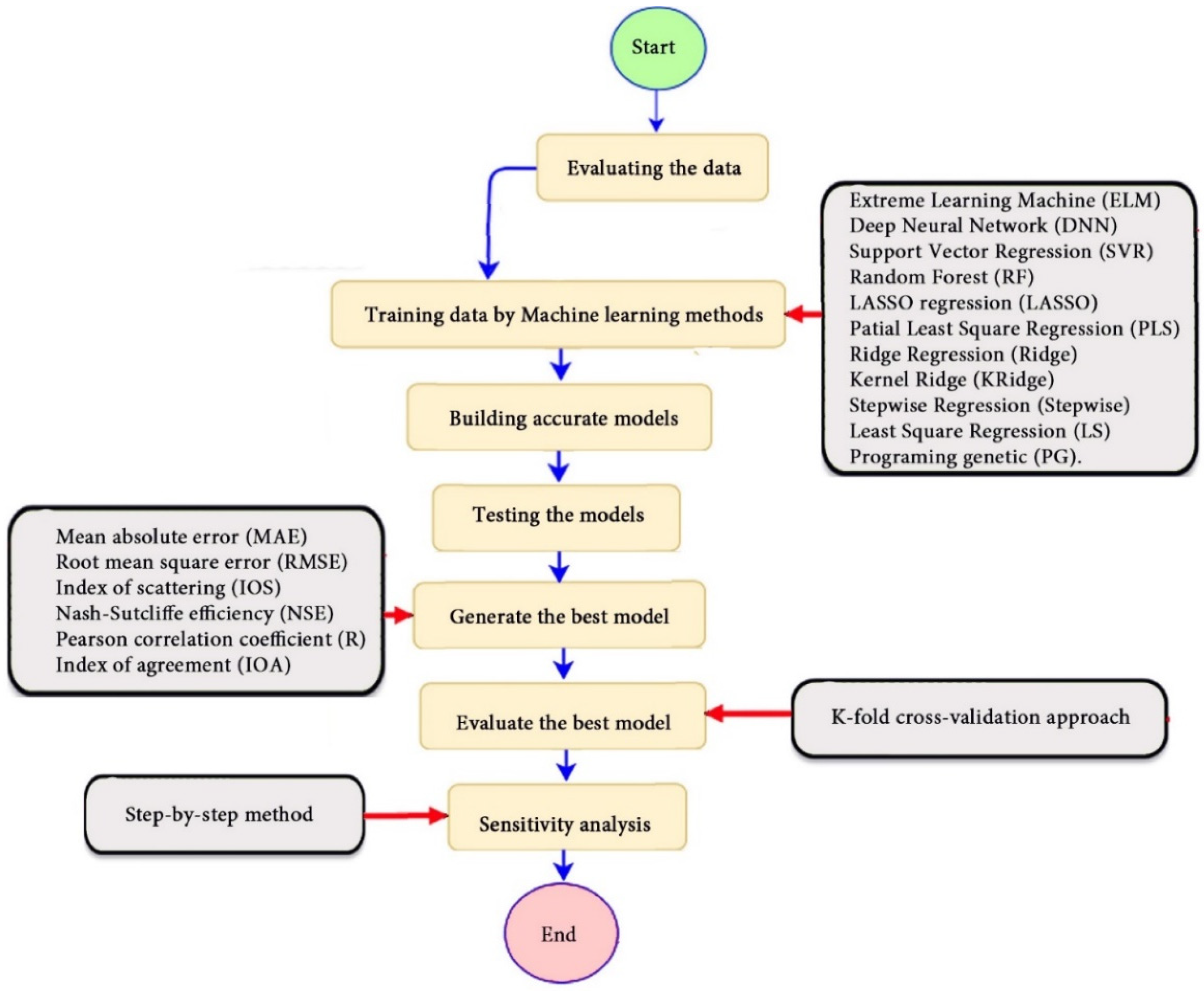
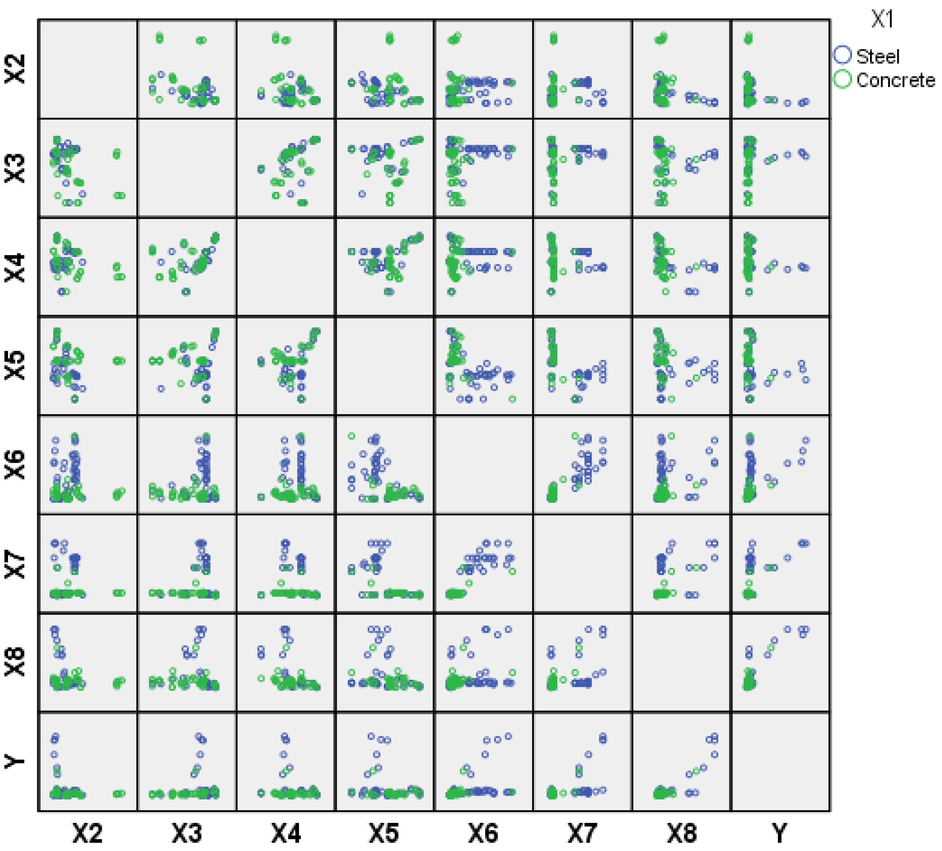
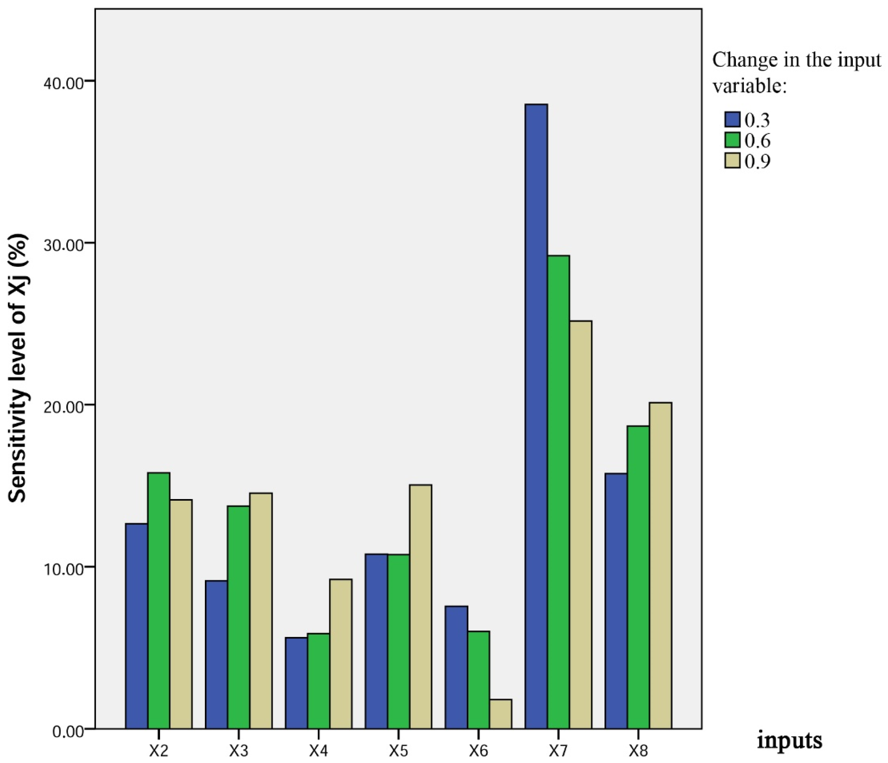
In the current study, a very important contribution in the geotechnical community has been introduced for the sake of enhancing the performance of the pile-bearing capacity model. It is worth mentioning here that the model quality is influenced by the method utilized. Hence, other unused advanced machine-learning methods demonstrated efficient results in other areas. Consequently, in the current study, we examined the usage of twelve advanced machine-learning methods, such as Deep Neural Network (DNN), Extreme Learning Machine (ELM), Support Vector Regression (SVR), LASSO regression (LASSO), Random Forest (RF), Ridge Regression (Ridge), Partial Least Square Regression (PLS), Stepwise Regression (Stepwise), Kernel Ridge (KRidge), Genetic Programming (GP), and Least Square Regression (LSR), to predict the pile-bearing capacity. According to the authors’ knowledge, the use of the aforementioned machine-learning methods in predicting the pile-bearing capacity is very rare. Therefore, this study began with collecting a wide range of data consisting of 100 static load-bearing tests on the UBC of both steel- and concrete-driven piles from different countries, such as Iran, Mexico, and India. Afterward, we selected eight relevant factors based on the literature recommendations, such as average cohesion (kN/m²), average friction angle (°), average soil-specific weight (kN/m³), average pile-soil friction angle (°), flap number, pile area (m²), and pile length (m). Based on that, eleven advanced machine-learning methods (DNN, ELM, SVR, LASSO, RF, Ridge, PLS, Stepwise, KRidge, GP, and LS) were applied for modeling the selected optimal input set for the first time. The findings clearly indicate that the Deep Neural Network (DNN) presents the most appropriate model, which yielded the minimum values of error metrics (MEA, RMSE, and IOS) and the higher values of R², R, and IOA compared to other models. Furthermore, the newly developed model was assessed by the K-fold cross-validation method and compared to other proposed models from the literature based on the correlation coefficient. The conclusion drawn is that the optimal DNN model could produce new data without causing over-fitting or under-fitting, plus being much more precise than the other proposed empirical models. Moreover, the last part in the current study consisted of the sensitivity analysis, which provided an overview of the most influential parameters on the pile-bearing capacity according to the proposed model. The findings indicate that the pile area was the most influential factor on the pile-bearing capacity. Pile length also had a considerable effect. In addition, the cohesion and friction angle demonstrated a moderate effect on the pile-bearing capacity, with a sensibility ratio ranging between 9% and 15%. Finally, the proposed optimal model was then used to develop a GUI public interface in order to facilitate its usage in the future. A reliable, easy-to-use, and graphical interface, named “BeaCa2021, presented in the current study, was programmed via Matlab software. The essential advantage of “BeaCa2021” is to help researchers and civil engineers interested in the problem of modeling regardless of their proficiency, by offering them plenty of benefits, such as reliability, easiness, and lowering the budget used for predicting the pile-bearing capacity from relevant and easily obtained parameters without the need to operate expensive in situ tests.

The results obtained in the current study also proved that the performance of the pile-bearing capacity model was considerably enhanced by using new machine-learning methods. The model prediction by the DNN was improved by 8.91% with the ANN method proposed by Nawari et al. [25], 3.58% with the PSO–ANN method proposed by Jahed et al. [1], and 0.86% with the MLP–GWO method proposed by Dehghanbanadaki et al. [30]. The obtained results are logical because deep learning is generally employed either in the prediction or in the problematic classification, which can reduce the bias and variance plus avoiding over-fitting and under-fitting problems, as opposed to the traditional ANN methods, to improve their predictive capability. According to these data, we can infer that the DNN method, which was employed in this study for the first time for the purpose of modeling the pile-bearing capacity, could yield more effective and accurate results than the other machine-learning methods.

Despite the multiple extraordinary findings of this study, a number of important limitations need to be addressed. The fundamental limitation would be the fact that the sample size was relatively small, which may affect the precision of the pile-bearing capacity. This may lead to the proposed model’s inability to generalize the new conditions or circumstances that were not used in the training data stage. Besides, researchers generally utilize large and diverse data collected by transferring knowledge between them. This is an important issue to build on in future research, i.e., to rely on the data gathered from multiple countries to enhance its learning and, therefore, produce a better model. Additionally, further studies using meta-heuristic algorithms for the prediction of pile-bearing capacity are strongly recommended. We mention, for example, the Particle Swarm Optimization (PSO) and Gravitational Search Algorithm (GSA), Bee Colony Algorithm (BCA), Bio-geography-Based Optimization (BBO), Whale Optimization Algorithm (WOA), Ant Colony Optimization (ACO), and Grey Wolf Optimizer (GWO). These algorithms have shown high-performance results when combined with machine-learning techniques, leading to improving their learning, and therefore rapidly converging to the best solution. The application of these meta-heuristic algorithms combined with machine-learning methods has shown impressive results in the abroad fields [55,61].

5. Conclusions

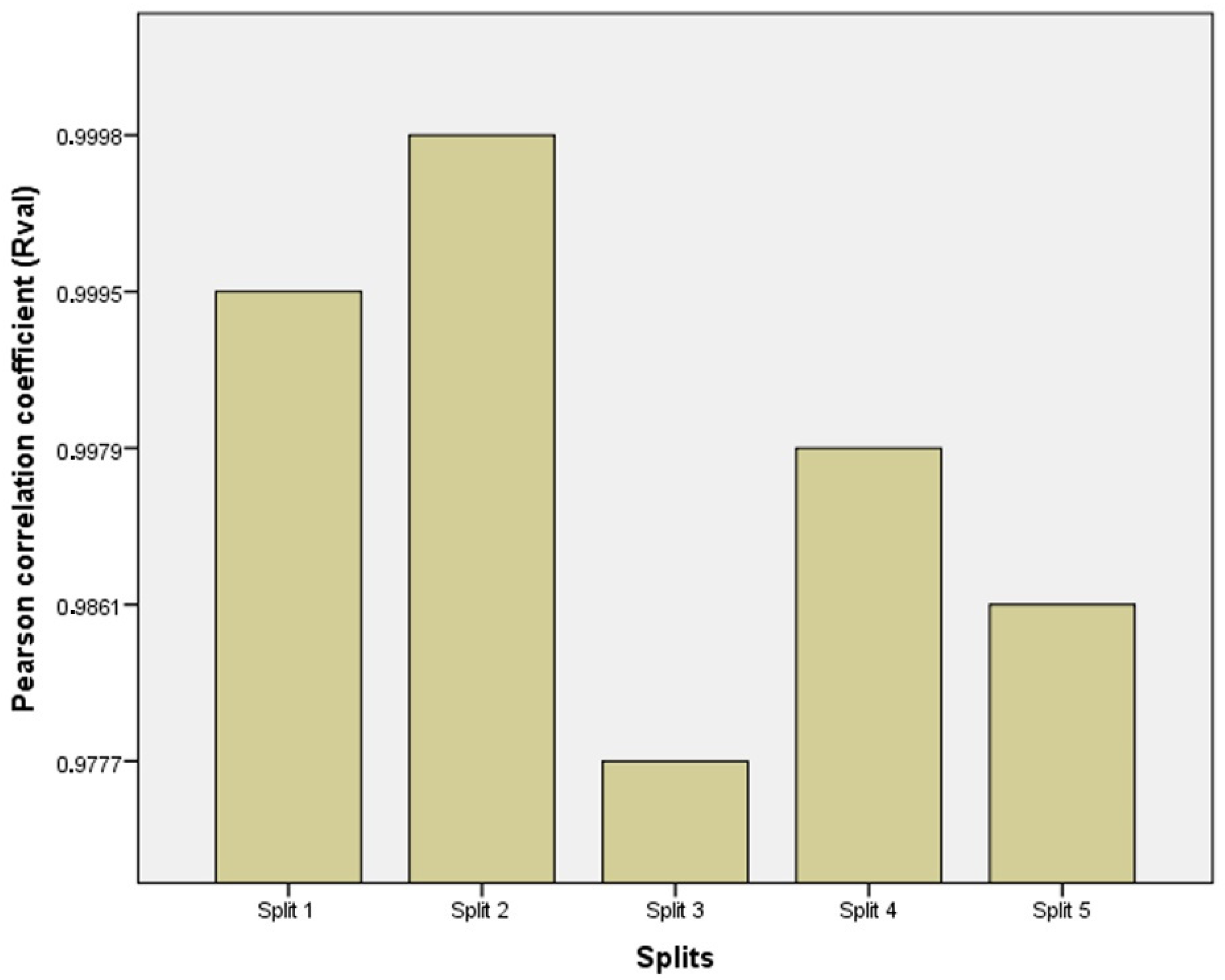
This study relied on a considerable number of steel- and concrete-driven pile data collected from different countries, such as Iran, Mexico, and India. The comparison of the results’ assessment between the different proposed models revealed the superiority of the DNN model proposed in our study, which yielded the highest accuracy in terms of MAE, RMSE, IOS, R, R², and IOA in both the training/validation phases. The findings indicate that this model has a high correlation coefficient, ranging between 0.9777 and 0.9998 for the validation data in the 5 splits of the k-fold cross-validation approach, meaning that there was no over-fitting or under-fitting. Furthermore, the results indicated that the aforementioned DNN model is more effective compared to other empirical models proposed in the literature. The sensitivity analysis results proved that pile area had the most significant effect on the prediction of the pile-bearing capacity. Pile lengths had a moderate influence and were ranked second. In addition, cohesion and friction angle had little effect on the pile-bearing capacity. Finally, the proposed optimal model was then used to develop a GUI public interface with Matlab software, named “BeaCa2021”. The fundamental benefit of “BeaCa2021” is to help researchers and practicing civil engineers, regardless of their proficiency, interested in the problem of modeling, to estimate the pile-bearing capacity with the benefits of gaining time and money.

This work has opened up several questions that need further investigations to overcome certain limitations. Firstly, there is a need to use more data from other countries to enhance the learning phase, which is needed to develop the BeaCa2021 in the future. Secondly, we propose the usage of meta-heuristic algorithms combined with machine-learning methods for predicting the pile-bearing capacity in future studies. These algorithms have demonstrated high-performance results when used with machine-learning techniques, leading to improved learning.

References

1. Jahed Armaghani, D.; Shoib, R.S.N.S.B.R.; Faizi, K.; Rashid, A.S.A. Developing a hybrid PSO–ANN model for estimating the ultimate bearing capacity of rock-socketed piles. Neural Comput. Appl. 2017, 28, 391–405. [Google Scholar] [CrossRef]
2. Yong, W.; Zhou, J.; Jahed Armaghani, D.; Tahir, M.M.; Tarinejad, R.; Pham, B.T.; Van Huynh, V. A new hybrid simulated annealing-based genetic programming technique to predict the ultimate bearing capacity of piles. Eng. Comput. 2021, 37, 2111–2127. [Google Scholar] [CrossRef]
3. Niazi, F.S.; Mayne, P.W. CPTu-based enhanced UniCone method for pile capacity. Eng. Geol. 2016, 212, 21–34. [Google Scholar] [CrossRef]
4. Meyerhof, G.G. Bearing Capacity and Settlement of Pile Foundations. J. Geotech. Eng. Div. 1976, 102, 197–228. [Google Scholar] [CrossRef]
5. Coyle, H.M.; Castello, R.R. New Design Correlations for Piles in Sand. J. Geotech. Eng. Div. 1981, 107, 965–986. [Google Scholar] [CrossRef]
6. Shahin, M.A. Intelligent computing for modeling axial capacity of pile foundations. Can. Geotech. J. 2010, 47, 230–243. [Google Scholar] [CrossRef] [Green Version]
7. Cai, G.; Liu, S.; Puppala, A.J. Reliability assessment of CPTU-based pile capacity predictions in soft clay deposits. Eng. Geol. 2012, 141–142, 84–91. [Google Scholar] [CrossRef]
8. Cai, G.; Liu, S.; Tong, L.; Du, G. Assessment of direct CPT and CPTU methods for predicting the ultimate bearing capacity of single piles. Eng. Geol. 2009, 104, 211–222. [Google Scholar] [CrossRef]
9. Eslami, A.; Heidarie Golafzani, S. Relevant data-based approach upon reliable safety factor for pile axial capacity. Mar. Georesour. Geotechnol. 2020, 39, 1373–1386. [Google Scholar] [CrossRef]
10. Momeni, E.; Nazir, R.; Jahed Armaghani, D.; Maizir, H. Prediction of pile bearing capacity using a hybrid genetic algorithm-based ANN. Measurement 2014, 57, 122–131. [Google Scholar] [CrossRef]
11. D18 Committee. Test Method for High-Strain Dynamic Testing of Deep Foundations; ASTM International: West Conshohocken, PA, USA, 2008. [Google Scholar]
12. Berezantzev, V.G. Design of deep foundations. In Proceedings of the Proc. 5th ICSMFE, Montreal, QC, Canada, 11–13 September 1965. [Google Scholar]
13. Hansen, J.B. Simple statical computation of permissible pileloads. Christ. Nielsen Post 1951, 12, 14–17. [Google Scholar]
14. De Beer, E.E. Etude des fondations sur pilotis et des fondations directes. Ann. Trav. Publics Belqique 1945, 46, 1–78. [Google Scholar]
15. Vesic, A.S. Design of pile foundations. In NCHRP Synthesis of Highway Practice; Transportation Research Board: Washington, DC, USA, 1977. [Google Scholar]
16. Abu-Farsakh, M.Y.; Titi, H.H. Assessment of Direct Cone Penetration Test Methods for Predicting the Ultimate Capacity of Friction Driven Piles. J. Geotech. Geoenvironmental Eng. 2004, 130, 935–944. [Google Scholar] [CrossRef]
17. Kordjazi, A.; Pooya Nejad, F.; Jaksa, M.B. Prediction of ultimate axial load-carrying capacity of piles using a support vector machine based on CPT data. Comput. Geotech. 2014, 55, 91–102. [Google Scholar] [CrossRef]
18. Maizir, H.; Suryanita, R.; Jingga, H. Estimation of pile bearing capacity of single driven pile in sandy soil using finite element and artificial neural network methods. In Proceedings of the International Conference on Engineering and Technology, Computer, Basic and Applied Sciences ECBA, Osaka, Japan, 28–29 November 2016. [Google Scholar]
19. Graine, N.; Hjiaj, M.; Krabbenhoft, K. 3D failure envelope of a rigid pile embedded in a cohesive soil using finite element limit analysis. Int. J. Numer. Anal. Methods Geomech. 2021, 45, 265–290. [Google Scholar] [CrossRef]
20. Conte, E.; Pugliese, L.; Troncone, A.; Vena, M. A Simple Approach for Evaluating the Bearing Capacity of Piles Subjected to Inclined Loads. Int. J. Geomech. 2021, 21, 04021224. [Google Scholar] [CrossRef]
21. Debiche, F.; Kettab, R.M.; Benbouras, M.A.; Benbellil, B.; Djerbal, L.; Petrisor, A.-I. Use of GIS systems to analyze soil compressibility, swelling and bearing capacity under superficial foundations inalgiers region, ALGERIA. Urban. Arhit. Constr. 2018, 9, 357–370. [Google Scholar]
22. Ikeagwuani, C.C. Estimation of modified expansive soil CBR with multivariate adaptive regression splines, random forest and gradient boosting machine. Innov. Infrastruct. Solut. 2021, 6, 199. [Google Scholar] [CrossRef]
23. Shahin, M.A.; Jaksa, M.B.; Maier, H.R. State of the art of artificial neural networks in geotechnical engineering. Electron. J. Geotech. Eng. 2008, 8, 1–26. [Google Scholar]
24. Benbouras, M.A.; Kettab, R.M.; Zedira, H.; Petrisor, A.-I.; Debiche, F. Dry density in relation to other geotechnical proprieties of Algiers clay. Rev. Şcolii Dr. Urban. 2017, 2, 5–14. [Google Scholar]
25. Nawari, N.O.; Liang, R.; Nusairat, J. Artificial intelligence techniques for the design and analysis of deep foundations. Electron. J. Geotech. Eng. 1999, 4, 1–21. [Google Scholar]
26. Mahesh, P. Modeling pile capacity using generalized regression neural network. In Proceedings of the Indian Geotechnical Conference, Kochi, India, 15–17 December 2011; No. N-027. pp. 811–814. [Google Scholar]
27. Milad, F.; Kamal, T.; Nader, H.; Erman, O.E. New method for predicting the ultimate bearing capacity of driven piles by using Flap number. KSCE J. Civ. Eng. 2015, 19, 611–620. [Google Scholar] [CrossRef]
28. Moayedi, H.; Raftari, M.; Sharifi, A.; Jusoh, W.A.W.; Rashid, A.S.A. Optimization of ANFIS with GA and PSO estimating α ratio in driven piles. Eng. Comput. 2020, 36, 227–238. [Google Scholar] [CrossRef]
29. Shaik, S.; Krishna, K.S.R.; Abbas, M.; Ahmed, M.; Mavaluru, D. Applying several soft computing techniques for prediction of bearing capacity of driven piles. Eng. Comput. 2019, 35, 1463–1474. [Google Scholar] [CrossRef]
30. Harandizadeh, H.; Jahed Armaghani, D.; Khari, M. A new development of ANFIS–GMDH optimized by PSO to predict pile bearing capacity based on experimental datasets. Eng. Comput. 2021, 37, 685–700. [Google Scholar] [CrossRef]
31. Moayedi, H.; Jahed Armaghani, D. Optimizing an ANN model with ICA for estimating bearing capacity of driven pile in cohesionless soil. Eng. Comput. 2018, 34, 347–356. [Google Scholar] [CrossRef]
32. Kardani, N.; Zhou, A.; Nazem, M.; Shen, S.-L. Estimation of Bearing Capacity of Piles in Cohesionless Soil Using Optimised Machine Learning Approaches. Geotech. Geol. Eng. 2020, 38, 2271–2291. [Google Scholar] [CrossRef]
33. Liu, L.; Moayedi, H.; Rashid, A.S.A.; Rahman, S.S.A.; Nguyen, H. Optimizing an ANN model with genetic algorithm (GA) predicting load-settlement behaviours of eco-friendly raft-pile foundation (ERP) system. Eng. Comput. 2020, 36, 421–433. [Google Scholar] [CrossRef]
34. Dehghanbanadaki, A.; Khari, M.; Amiri, S.T.; Armaghani, D.J. Estimation of ultimate bearing capacity of driven piles in c-φ soil using MLP-GWO and ANFIS-GWO models: A comparative study. Soft Comput. 2021, 25, 4103–4119. [Google Scholar] [CrossRef]
35. Alavi, A.H.; Gandomi, A.H.; Mollahasani, A.; Bazaz, J.B. Linear and tree-based genetic programming for solving geotechnical engineering problems. In Metaheuristics in Water, Geotechnical and Transport Engineering; Elsevier: Amsterdam, The Netherlands, 2013; pp. 289–310. ISBN 978-0-12-398296-4. [Google Scholar]
36. Narendra, B.S.; Sivapullaiah, P.V.; Suresh, S.; Omkar, S.N. Prediction of unconfined compressive strength of soft grounds using computational intelligence techniques: A comparative study. Comput. Geotech. 2006, 33, 196–208. [Google Scholar] [CrossRef]
37. Rezania, M.; Javadi, A.A. A new genetic programming model for predicting settlement of shallow foundations. Can. Geotech. J. 2007, 44, 1462–1473. [Google Scholar] [CrossRef]
38. Stockard, D.M. Case Histories-Pile Driving in the Gulf of Mexico; OnePetro: Houston, TX, USA, 1979. [Google Scholar]
39. Stockard, D.M. Case Histories: Pile Driving Offshore India; OnePetro: Houston, TX, USA, 1986. [Google Scholar]
40. Tucker, L.M.; Briaud, J.-L. Analysis of the Pile Load Test Program at the Lock and Dam 26 Replacement Project; Texas A&M University College Station Dept of Civil Engineering: College Station, TX, USA, 1988. [Google Scholar]
41. Gupta, R.C. Estimating Bearing Capacity Factors and Cone Tip Resistance. J. Jpn. Geotech. Soc. 2002, 42, 117–127. [Google Scholar] [CrossRef] [Green Version]
42. Fellenius, B.H.; Altaee, A. Pile dynamics in geotechnical practice—six case histories. In Deep Foundations 2002: International Perspective Theory Design, Construction Perform; American Society of Civil Engineers: Reston, VA, USA, 2012; pp. 619–631. [Google Scholar] [CrossRef] [Green Version]
43. Benbouras, M.A.; Kettab Mitiche, R.; Zedira, H.; Petrisor, A.I.; Mezouar, N.; Debiche, F. A new approach to predict the Compression Index using Artificial Intelligence Methods. Mar. Georesources Geotechnol. 2019, 37, 704–720. [Google Scholar] [CrossRef]
44. Benbouras, M.A.; Kettab, R.M.; Zedira, H.; Debiche, F.; Zaidi, N. Comparing Nonlinear Regression Analysis And Artificial Neural Networks To Predict Geotechnical Parameters From Standard Penetration Test. Urban. Archit. Constr. Arhit. Constr. 2018, 9, 275–288. [Google Scholar]
45. Huang, G.-B.; Zhu, Q.-Y.; Siew, C.-K. Extreme learning machine: Theory and applications. Neurocomputing 2006, 70, 489–501. [Google Scholar] [CrossRef]
46. Biau, G.; Scornet, E. A random forest guided tour. Test 2016, 25, 197–227. [Google Scholar] [CrossRef] [Green Version]
47. Awad, M.; Khanna, R. Support vector regression. In Efficient Learning Machines: Theories, Concepts, and Applications for Engineers and System Designers; Awad, M., Khanna, R., Eds.; Apress: Berkeley, CA, USA, 2015; pp. 67–80. ISBN 978-1-4302-5990-9. [Google Scholar]
48. Vinzi, V.E.; Chin, W.W.; Henseler, J.; Wang, H. Editorial: Perspectives on partial least squares. In Handbook of Partial Least Squares: Concepts, Methods and Applications; Springer Handbooks of Computational Statistics; Esposito Vinzi, V., Chin, W.W., Henseler, J., Wang, H., Eds.; Springer: Berlin/Heidelberg, Germany, 2010; pp. 1–20. ISBN 978-3-540-32827-8. [Google Scholar]
49. Hebiri, M.; Lederer, J. How Correlations Influence Lasso Prediction. IEEE Trans. Inf. Theory 2013, 59, 1846–1854. [Google Scholar] [CrossRef] [Green Version]
50. Douak, F.; Melgani, F.; Benoudjit, N. Kernel ridge regression with active learning for wind speed prediction. Appl. Energy 2013, 103, 328–340. [Google Scholar] [CrossRef]
51. Hoerl, A.E.; Kennard, R.W. Ridge Regression—1980: Advances, Algorithms, and Applications. Am. J. Math. Manag. Sci. 1981, 1, 5–83. [Google Scholar] [CrossRef]
52. Jennrich, R.I.; Sampson, P.F. Application of Stepwise Regression to Non-Linear Estimation. Technometrics 1968, 10, 63–72. [Google Scholar] [CrossRef]
53. Wagner, S.; Kronberger, G.; Beham, A.; Kommenda, M.; Scheibenpflug, A.; Pitzer, E.; Vonolfen, S.; Kofler, M.; Winkler, S.; Dorfer, V.; et al. Architecture and design of the HeuristicLab optimization environment. In Advanced Methods and Applications in Computational Intelligence; Topics in Intelligent Engineering and Informatics; Klempous, R., Nikodem, J., Jacak, W., Chaczko, Z., Eds.; Springer International Publishing: Berlin/Heidelberg, Germany, 2014; pp. 197–261. ISBN 978-3-319-01436-4. [Google Scholar]
54. Tikhamarine, Y.; Malik, A.; Pandey, K.; Sammen, S.S.; Souag-Gamane, D.; Heddam, S.; Kisi, O. Monthly evapotranspiration estimation using optimal climatic parameters: Efficacy of hybrid support vector regression integrated with whale optimization algorithm. Environ. Monit. Assess. 2020, 192, 696. [Google Scholar] [CrossRef] [PubMed]
55. Amin Benbouras, M.; Petrisor, A.-I. Prediction of Swelling Index Using Advanced Machine Learning Techniques for Cohesive Soils. Appl. Sci. 2021, 11, 536. [Google Scholar] [CrossRef]
56. Breiman, L.; Spector, P. Submodel Selection and Evaluation in Regression. The X-Random Case. Int. Stat. Rev. Rev. Int. Stat. 1992, 60, 291–319. [Google Scholar] [CrossRef]
57. Oommen, T.; Baise, L.G. Model development and validation for intelligent data collection for lateral spread displacements. J. Comput. Civ. Eng. 2010, 24, 467–477. [Google Scholar] [CrossRef]
58. Goetz, J.N.; Brenning, A.; Petschko, H.; Leopold, P. Evaluating machine learning and statistical prediction techniques for landslide susceptibility modeling. Comput. Geosci. 2015, 81, 1–11. [Google Scholar] [CrossRef]
59. Amin, B. Predicting Shear Stress Parameters in Consolidated Drained Conditions Using Artificial Intelligence Methods. Basic Appl. Sci.-Sci. J. King Faisal Univ. 2021, 22, 1–7. [Google Scholar] [CrossRef]
60. Liong, S.-Y.; Lim, W.-H.; Paudyal, G.N. River Stage Forecasting in Bangladesh: Neural Network Approach. J. Comput. Civ. Eng. 2000, 14, 1–8. [Google Scholar] [CrossRef]
61. El Amin Bourouis, M.; Zadjaoui, A.; Djedid, A. Contribution of two artificial intelligence techniques in predicting the secondary compression index of fine-grained soils. Innov. Infrastruct. Solut. 2020, 5, 96. [Google Scholar] [CrossRef]
Figure 1. Flowchart describing the key steps for the methodology of research to estimate the pile-bearing capacity.
Applsci 11 10908 g001
Figure 2. The correlation matrix between the pile-bearing capacity and soil parameters (green points: concrete material; blue points: steel material).
Applsci 11 10908 g002
Figure 3. Performance measures of the DNN model using the K-fold cross-validation, with K = 5.
Applsci 11 10908 g003
Figure 4. Results of the sensitivity analysis of the proposed model.
Applsci 11 10908 g004
Figure 5. BeaCa2021 interface.
Applsci 11 10908 g005