1. Introduction
Intelligent models are expected to play a key role in accomplishing the goals of Industry 4.0, which include the evolution of traditional manufacturing systems into intelligent, automated systems. In this context, research on machine and deep learning has rapidly dominated applications within the industrial field, especially in the current second level of Industry 4.0, which is data and intelligence driven [
1]. Despite such an apparent success, machine learning-based solutions deployed into real industrial applications are still few and mostly conducted by a small group of predominantly large companies [
2]. According to Bertolini et al. [
2], production planning and control and defect analysis are examples of emerging research topics that are already attracting significant academic and industrial interest which is expected to continue growing in the coming years.
Particularly in problems involving defect identification and classification, visual quality inspection is an important research topic, and images are among the most common type of data dealt with. Several studies have proposed solutions supported by automated image recognition using machine learning for defect detection, such as identifying material defects in the selective laser melting of metal powders [
3], and the defect classification of semiconductor fabrication using scanning electron microscope images [
4]. However, we note that the literature has given significantly less attention to the investigation of this kind of problem using video data.
Although different aspects addressed in works that investigate defect identification from images may be extremely useful when dealing with video, the latter poses unique challenges, especially when considering the spatio-temporal patterns of input video sequences. In addition, video data are difficult to represent and model due to their high dimensionality, the presence of noise, and the fact that each video segment may represent a wide variety of events.
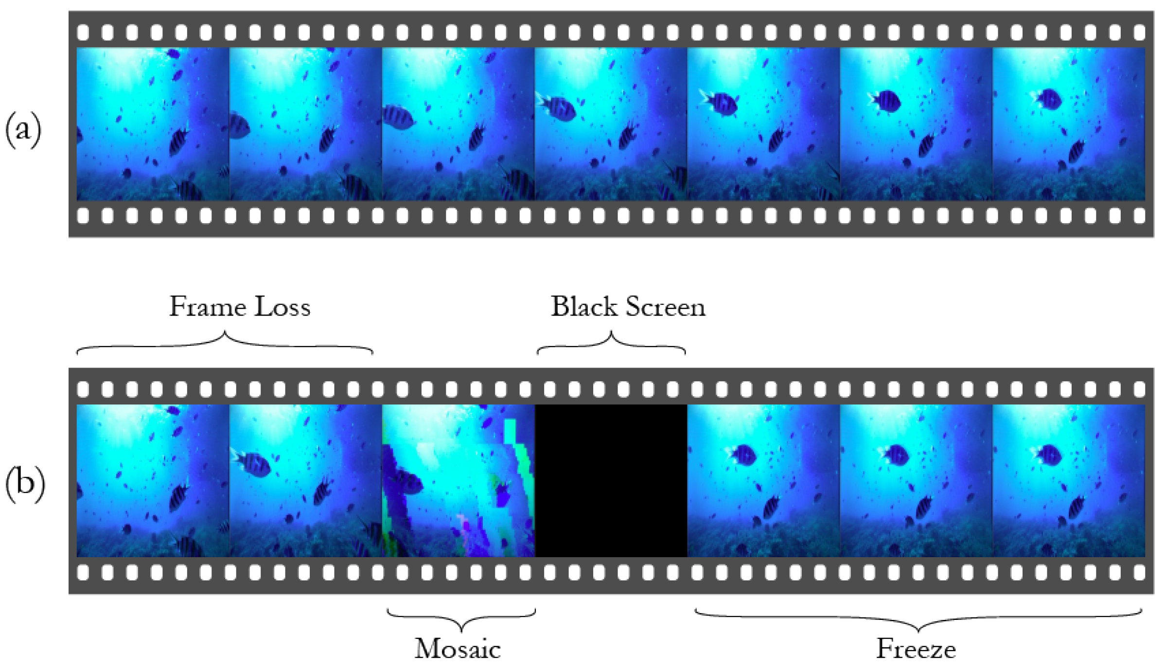
The problem investigated in this paper involves defect identification from video data. In the assembly line of a TV set manufacturer, the TV’s digital decoders must be tested to ensure that no defects occur. For instance, some possible defects are: (1) mosaic—characterized by artifacts of a geometric pattern which may partly or completely block the video’s frames; (2) freeze—corresponding to consecutive repetitions of the same frame; (3) frame loss—temporal jumps that skip more than a single frame at a time; and (4) black screen—when the complete darkening of the screen replaces one or more frames. In order to better illustrate these defects,
Figure 1 shows two different frame sequences, one with no anomalies (
Figure 1a) and another presenting all four defects (
Figure 1b).
Detecting defects in video may be considered a special case of video anomaly detection, since the objective of this task is usually to discriminate positive events from negative and rare ones. An anomaly is usually an outlier, a non-standard piece of data, such as defects in surfaces [
5]. Anomaly detection may be employed in a wide range of applications, such as the identification of noisy signals [
6], disease classification [
7,
8,
9], and pest control through environment surveillance [
10,
11]. Deep learning-based methods are considered the state-of-the-art in video anomaly detection [
12]. According to Nayak et al. [
12], among the categories of deep learning methods used for video anomaly detection, the most widely used are supervised and semi-supervised learning. In the first category, convolutional neural networks (CNNs) built with spatio-temporal layers—e.g., convolutional 3D or two-stream CNN—are successfully used as video descriptors to provide discriminative information when labeled data are available. In the second, spatio-temporal auto-encoders, based on convolutional long short-term memory (ConvLSTM) architecture for instance, are very popular. These models are trained in a one-class classification (OCC) fashion. Typically, the models are trained to reconstruct normal videos with high precision, and when presented to anomalies, they commit high reconstruction errors. That reconstruction error may be used to decide whether the input video is an anomaly or not.
Considering semi-supervised learning, more recent attention in the literature has been focused on the provision of adversarial training by adopting a generative adversarial network (GAN) within anomaly detection [
13]. In a typical GAN procedure, the generator provides fake samples and passes them to the discriminator, which focuses on distinguishing fake from real samples. The discriminator is trained to be as precise as possible in assigning correct labels to both real and fake samples, while the generator learns to provide fake samples realistic enough to confound the discriminator. In the context of anomaly detection, however, the process is slightly different. The common procedure is to train one standard GAN using the OCC approach. Hence, only non-anomaly samples are used to lead the GAN to learn a mapping from the latent space representation to the samples. Therefore, the generator learns how to generate normal samples. In test time, since each sample needs to be mapped to the latent space, when an anomalous sample is encoded, a high discrimination score is expected, while a low score is likely to be indicative of a non-anomalous sample. It is important to mention that some recent studies present methods that use both GAN and autoencoders for anomaly detection, as in [
14].
Semi-supervised approaches are particularly interesting for defect detection because they exploit the fact that normal video instances are usually largely available in real applications, while collecting defect data with sufficient variety, volume, and quality is generally costly and time-consuming. However, the lack of anomalous samples for validation may be a drawback to this strategy. GANs can mitigate this problem as they may successfully generate anomalous samples [
13]. Some examples of works proposing GANs to solve the imbalanced data problem in the manufacturing domain are [
15,
16,
17]. In terms of videos, acquiring enough anomalous data is even harder. Consequently, common supervised deep learning neural network training tasks cannot be carried out. Instead, GANs may be used to generate the samples of anomalous videos.
In this work, we proposed a novel GAN-based anomaly detection model which learns to generate samples of anomalous video in a semi-supervised way. The proposed method requires only normal data and few instances of the non-anomalous class in the training process. Unlike the traditional GAN whose generator component is composed of fractional convolutional layers and its loss is calculated by taking into account the discriminator’s classification, we propose a custom generator component to generate synthetic anomalous instances from the normal instances. This is performed by inserting anomaly into normal video instances using transformations such as Gaussian noise, temporal jumps and freezing. The discriminator loss values are used as an adjustment factor by the generator. The lower the discriminator loss is, the smoother the defects produced by the generator are. As a consequence, the video samples used to train the discriminator become increasingly “harder” as the discriminator’s loss reduce during the training process. We do so because, as pointed by [
18], it is important that the discriminator and the generator learn simultaneously, unless the discriminator does not have ample gradients to update its weights with. Similarly, the generator must steadily show harder anomalies, otherwise it would not have a generator competing against the discriminator.
In addition, we introduce in this paper three novel video datasets that simulate real-world industry-oriented failures. The datasets provide video-level annotations, i.e., a video is labeled as anomalous or anomalous, but the timestamps of the anomalies within each video are unknown. We compare the results achieved by our proposed GAN against five different models. More specifically, four supervised methods: a custom 3D CNN, 3D ResNet-34 [
19], Mobile Video Networks (MoViNet-A2) [
20], and Convolution 3D (C3D) [
21]; and one semi-supervised method: an autoencoder model composed of residual blocks, ConvLSTM, and ConvCNN layers, recently proposed in [
22].
The remainder of this paper is organized as follows. A short review of the state-of-the-art involving spatio-temporal deep learning-based methods for video anomaly detection is presented in
Section 2. An in-depth description of the datasets created and the GAN proposed, as well as the additional models investigated in this paper, is provided in
Section 3.
Section 4 describes experiments and results. Finally, conclusions and future work are presented in
Section 5.
2. Related Work
In this section, we discuss works focused on detecting abnormal events in video, such as action recognition and surveillance videos. As mentioned in the introduction, the detection of abnormal events has attracted significant attention in the image processing domain [
23] but is not yet a much-explored research issue when video is involved—especially in the context of industrial applications. Moreover, the most popular approaches in the literature deal with three-dimensional (3D) data considering 2D images which may limit detecting temporal (motion) patterns. Therefore, the works described here are spatio-temporal models, i.e., they simultaneously focus on both spatial (appearance) and motion features, applied in different tasks. These works are divided into three categories: (1) CNN based; (2) autoencoders; and (3) GAN based.
2.1. CNN-Based Approaches
The first group of works adopted the most explored technique based on supervised learning, precisely CNN. These solutions may be divided into two approaches: two-stream CNN and 3D-CNN.
In [
24], Sha et al. proposed extracting spatial and temporal features separately using a two-stream CNN approach to detect abnormal behaviors in an electrical industry, such as “illegal cutting” and “running”. DenseNet is the base CNN architecture used in both spatial and temporal stream networks. The main difference between the two-stream network members is the input data. The spatial one is the traditional DenseNet working with 2D standard RGB image frame sequences, while optical flow (DeepFlow) is responsible for encoding motion information. The extracted optical flow is transformed into grayscale images and used as input to the temporal stream network. The loss function is focal loss, which is appropriate for training two-stream CNNs in the presence of imbalanced data. Considering the fact that two separate models are trained, the final decision is made using a weighted sum function to combine their predictions. The authors reported that this two-stream CNN approach performed better than traditional and other deep learning-based methods. It is also important to mention that the best fusion function trade-off was obtained by adopting a weight five times higher for the temporal stream network. However, even though optical flow is widely used to describe motion information, a 3D convolutional kernel may improve the extraction of temporal patterns.
This is the main focus in [
25], whose author proposed a two-stream 3D-CNN architecture to detect anomalous events in videos. This architecture is also a two-stream CNN approach composed of a network to handle spatial information and another one to handle temporal information. Here, however, both networks are 3D-CNNs. More precisely, the author employed the inflated 3D architecture (i3D) in each stream network. In this type of architecture, instead of directly creating a network with 3D convolutions, a 2D convolution network is used, inflating its filters and pooling kernels with the addition of a temporal dimension. The network responsible for the spatial information accepts an RGB video as input, whilst the member dealing with temporal information accepts an optical flow stream as input. Both networks were initialized with weights pre-trained on ImageNet and Kinetics databases—a large collection of video clips for human action recognition. The models were then trained and fine-tuned on a customized dataset created to represent several anomalous events, such as violence, loitering and falling. The final layer of each network is a Softmax layer used to provide predictions from both models to make a final decision, which is obtained by the weighted summing of each network’s prediction. The results showed that transfer learning from a related problem, e.g., action recognition, in addition to the use of 3D architectures, were the reasons for which this approach outperforms other architectures. On the other hand, optical flow is an expensive and time-consuming step, which could be avoided by directly extracting temporal information from raw data.
The work presented by Wei Lin et al. [
26] differs from the two previous approaches as it does not depend on optical flow. Moreover, rather than using i3D, they directly employ 3D convolutions. The authors proposed a 3D-CNN using 3D ResNet as base architecture to detect anomalous events in crowd scenes. This architecture works with convolution layers, adding an extra dimension to the convolution filters to deal with motion patterns in videos. In addition to 3D ResNet, the proposed method works with a self-attention mechanism to simultaneously capture temporal and spatial features. This mechanism is a non-local neural network. However, the model failed when tested on real data, since it was originally designed using a database composed of synthetic videos generated using scenes from the Grand Theft Auto V (GTA V) game. As a consequence, the authors applied a Cyclic 3D GAN to eliminate the difference between the source and target domains, which was performed using GAN to turn synthetic videos into realistic monitoring videos. The results showed that the proposed model was able to surpass the simple 3D ResNet adopted as the baseline, as well as other video classification models such as LSTM, in real and synthetic databases.
2.2. Autoencoders
Another popular approach to carry out anomaly detection in video is based on deep autoencoders. These methods are trained with normal data only and are categorized as semi-/weakly supervised approaches. The reconstruction error is used as a threshold to detect anomalies because it is expected that the reconstruction error will be lower for the normal data and higher for the abnormal data. We discussed in this section autoencoder models focused on providing spatio-temporal representations [
22].
In [
27], autoencoders are used to detect anomalies in various benchmark datasets such as anomaly detection in crowded scenes. The authors proposed two different autoencoders: (1) a fully connected one working with handcrafted features extracted to represent spatio-temporal information; and (2) a fully convolutional feed-forward autoencoder to learn spatio-temporal patterns and provide classification in an end-to-end learning framework. Handcrafted motion features consisting of histograms of oriented gradients (HOG) and histograms of optical flows (HOF) with improved trajectory capability are computed and fed as input to the first autoencoder. In its turn, the convolutional feed-forward autoencoder is designed to learn regular motion signatures directly from video, avoiding the work involved in handcrafting. This second autoencoder is composed of: an encoder containing three convolutional layers and two max pooling layers; and a decoder with a reverse encoder structure. Its input is a temporal cuboid obtained by stacking several frames together. The experimental results showed that both methods reached a competitive performance compared to other state-of-the-art anomaly detection methods. However, the convolutional autoencoder showed an advantage since it is not a handcrafted-based approach.
The architecture of convolutional autoencoders has evolved as a consequence of the evolution of different deep learning techniques. For instance, the authors in [
23] proposed a spatio-temporal architecture capable of detecting anomalies in video using convolutional long short-term memory (Conv.LSTM) in addition to a convolutional autoencoder (ConvAE). The additional component (Conv.LSTM) is responsible for providing both spatial and temporal information from the input videos. It is also an end-to-end trainable model whose architecture consists of two encoder–decoder components: (1) a spatial and (2) a temporal encoder–decoder. In the first, two convolution layers compose the encoder and there are two deconvolution layers in the decoder part. This first member is designed to learn the spatial structures of each video frame. The temporal encoder–decoder is placed in between the encoder and decoder components of the spatial autoencoder. It contains three Conv.LSTM layers for detecting the motion patterns of the encoded structures. The authors concluded that the Conv.LSTM layers were suitable to tackle the spatio-temporal data due to its inherent convolutional structure. They compared this architecture to methods based on 2D autocoders in various benchmark datasets. The results showed the proposed architecture was superior in detecting fewer false negatives. On the other hand, depending on the complexity of the handled video, the model may produce more false negatives.
ConvAE and Conv.LSTM are also components of the OF-ConvAE-LSTM [
28] method, proposed to detect unusual events in surveillance videos. The difference between OF-ConvAE-LSTM and the model proposed in [
23] is the use of a dense optical flow technique which is applied to assimilate the speed and direction information of the foreground objects. The dense optical flow map of each video frame was extracted as a pre-processing step and fed as input to the model. As in [
23], there are two encoder–decoder components (spatial and temporal) in this architecture. The ConvAE contains two convolution layers in the encoder and two deconvolution layers in the decoder. The Conv.LSTM layers (three) are in-between the spatial encoder and decoder parts. Again, the Conv.LSTM layers are expected to capture the temporal dynamics of video sequences along with spatial information. The experimental results indicated that OF-ConvAE-LSTM is effective in detecting anomalies in videos. In addition, the model was able to outperform the oldest approaches. However, as previously mentioned, optical flow increases the model complexity.
In [
22], a spatio-temporal residual autocoder (R-STAE) architecture was proposed to obtain visual patterns more accurately than other types of deep spatio-temporal autocoders. The R-STAE architecture is composed of layers common in other autocoder architectures used in video anomaly detection tasks such as: 3D convolution, deconvolution and Conv.LSTM layers. The difference in R-STAE are the residual blocks added to the architecture, used to avoid the vanishing gradient problem. The architecture is composed of three convolution layers and one Conv.LSTM layer in the encoder component, while the decoder consists of three deconvolution layers and one Conv.LSTM layer. The residual blocks are located between the encoder and decoder components. As the preceding methods, R-STAE is built as an end-to-end learning framework guided by the reconstruction loss. The experimental results on anomaly detection in surveillance videos showed that the addition of residual blocks to the network helps achieve lower reconstruction loss compared to the network with no residual blocks. In addition, R-STAE outperformed other methods considered state-of-the-art. However, due to the different types of layers involved, the setup of some hyperparameters is difficult and may critically affect the performance of the model. For instance, a very low number of hidden units in the Conv.LSTM layer can lead to information loss, whilst the opposite can introduce redundancy in the latent representation.
2.3. GAN Based
Generative adversarial networks (GANs) are gaining popularity in conducting anomaly detection tasks in a semi-supervised manner. They work by creating structures from normal data, which represents standard data distribution, since the generator is trained to reproduce normal data and the discriminator is used to discriminate normal from non-normal data. In the context of quality and/or defect classification tasks, GANs may be applied to increase the minority class of unbalanced datasets, as the so-called data-unbalancing problem is a typical issue in real industrial applications. In line with this objective, some works have explored the recent advancements in GAN-based approaches that enable these models to effectively generate synthetic training data as a way to augment scarce training sets in manufacturing quality control tasks. The works discussed in this section were mainly concerned with improving the generator to increase the generation quality, and consequently, the discriminators’ capability.
For instance, Peres et al. [
29] initially performed the traditional GAN approach, which involves training two networks simultaneously: one generator and one discriminator. The error signal provided to the discriminator is obtained from ground truth normal instances indicating whether a sample is real or synthetic. A similar error signal is used to train the generator (via the discriminator), enabling it to generate synthetic images with improved quality. The main difference in this work is that it addresses the problem of increasing data variety and volume in a manufacturing quality control task by applying transfer learning from StyleGAN2-ADA [
30]. StyleGAN2-ADA is the TensorFlow official GAN implementation, which provides a discriminator adapted with an augmentation mechanism with the aim of stabilizing training in limited data regimes, accelerating convergence and reducing data requirements. Their results have shown that the performance reached by the models trained on the balanced dataset augmented using GANs was not only superior but also much more harmonized across all classes. Nonetheless, this method was designed to handle 2D data, which may be deemed to be a limitation, due to the fact that 2D-based approaches tend to ignore temporal structures.
It is worth noting that GANs can be employed to efficiently generate and reconstruct videos, reconstruct 3D objects from 2D data and even generate complete 3D models. In [
31], the authors presented an efficient framework able to generate 3D object shapes. In this work, a 3D-Mask-GAN was used to predict 3D structures from a single-view image. The framework is composed of three major steps: (1) one image encoder responsible for receiving a 2D image, which should be compressed and processed; (2) one generator, whose output is a 3D object created from the 2D input image; and (3) one discriminator network to distinguish real masks from generated ones. This work differs from previous methods as the generator is followed by a projector which works with a 4-by-4 transformation matrix that includes a camera calibration matrix and extrinsic parameters to create 2D masks to be fed as input to the discriminator. Consequently, the discriminator evaluates the masks provided by the projector instead of a 3D volume. Even though this method manages to recreate 3D volumes from 2D shapes, only isolated objects were concerned, such as the chair, car, plane, etc. This may lead to drawbacks when the entire 3D-scene evaluation is intended.
Enhancers are important alternatives in this case. These methods try to improve existing models by using GANs to iteratively enhance raw 3D reconstructed models using meshes and textures, for instance. One example is 3D-Scene-GAN, proposed in [
32]. It is a weakly semi-supervised framework (labeled real-time 2D images are used) that may be applied to successfully generate very complicated 3D reconstructed scenes. As in several current works, the traditional architecture of generator and discriminator models was used. However, the authors employed a distinct use of data acquisition and processing. 3D-Scene-GAN works by obtaining 2D scene images from reconstructed 3D scenes to make up pairs of 2D images from reconstructed and real 3D scenes in order to improve the discriminator model. To obtain the 2D images from the reconstructed scenes, the reconstructed 3D model is imported into the Blender and OpenDR [
33]. A virtual camera was setup in the Blender with optical parameters as a real camera to collect 2D images along the real camera trajectory. OpenDR is responsible for mapping 3D models to 2D images. The results indicated the superior performance of 3D-Scene-GAN when compared to state-of-the-art 3D reconstruction methods. On the other hand, the required real-time 2D images may be an expensive and time-consuming step.
Similarly to previously mentioned works, in this paper, we also employed GAN to augment and generate virtually unlimited synthetic training data. Despite being able to create non-anomalous video instances similar to the target class, a traditional three-dimensional generator creates non-accurate anomalous videos, especially due to the fact that some errors, e.g., freezing, black screen and mosaic, can occur at very short intervals. These limitations of traditional generators, as well as current works available in the literature, motivated us to propose in this paper an artificial generator to reproduce online anomalies closer to real anomalies. Our discriminator was designed to learn how to differentiate between anomaly and normal videos, instead of differentiating between fake and real instances. The proposed method is detailed in the next section.
3. Materials and Methods
We describe in this section the datasets generated to evaluate the models employed in this work. Then, we present the proposed GAN as well as other investigated methods.
3.1. Datasets
We introduced in this paper three novel video datasets that simulate real-world industry-oriented failures. The datasets are called 60frames, DenserGlitch and The_1R—listed in their chronological order of acquisition and complexity. Aiming to generate videos representing the real use-case scenario, the 60frames dataset represents the most controlled environment since its instances were obtained frame-by-frame. The instances of the remaining datasets were obtained in real time as the videos were played in one of the devices used.
All three datasets contain instances from two classes: (1) regular video segments; and (2) anomalous ones. All samples were generated from a single base video composed of 2399 frames sampled at 30 frames per second, leading to roughly 79 s of duration. The videos were collected in a controlled environment similar to the one used in the assembly line producing TV sets. To increase the variability of the data, two different television manufacturers and screen sizes were used, and the camera was moved around several times during the capture. It must be noted that none of the datasets contain any real anomaly. The defects were simulated based on observations of real anomalies. The details pertaining to each dataset are presented below.
3.1.1. 60frames
A camera Basler acA2500-14uc USB 3.0 equipped with C125-0418-5M-P f4mm lens was used to generate instances for this dataset. Each frame of the original video was displayed in the television’s screen and captured by the camera before changing to the next frame. Taking into account the fact that there were originally 2399 frames, 47,980 frames were collected for each class, since 10 camera positions were used for each of the two devices (32-inch and 43-inch screen size). The original resolution of the captured images is . However, the following preprocessing steps were conducted: crop—to only preserve the pixels inside the screen, obtaining an ROI with roughly pixels; and resize to . Only one type of anomaly (mosaic) was simulated before the instances’ capture. Each capture alternated between original frames and frames with the simulated mosaic so that later on, while constructing the videos, it was possible to insert other defects in any desired position, allowing the full control of where the anomalies would be placed and how long they would last.
Defective frames with mosaic were simulated using the glitch-this module, version 1.0.2, randomly alternating the glitches’ intensity between levels 2 and 10. Freezes, by adding multiple copies of a given frame, and darkened frames are examples of additional defects simulated after the frames’ capture. In addition, the defects’ duration was randomly chosen according to a normal distribution with a mean of 12 and standard deviation of 4, to determines the number of defective frames for each anomaly event. Finally, the produced frames provided 6240 video segments—among which precisely 4680 are anomalous instances (75%) and 1560 are normal (25%). Each video is composed of 60 frames, in order to increase the amount of examples for each class, and the last 30 frames of each sample overlap with the first 30 samples of the next one. As a consequence, the dataset was partitioned into training, validation and test sets, taking the frames shared by different videos of the same camera position into account so that all instances collected with a given camera position were placed in the same partition.
3.1.2. DenserGlitch
For this dataset, a Basler acA1300-200uc camera was employed due to the need to collect all frames using 30 frames per second as the sample rate. As a consequence of this change, the resolution of the captured frames decreased to
. The mosaic simulation procedure is also different since it is based on real anomalous instances obtained through experiments with signal attenuation performed to induce defects.
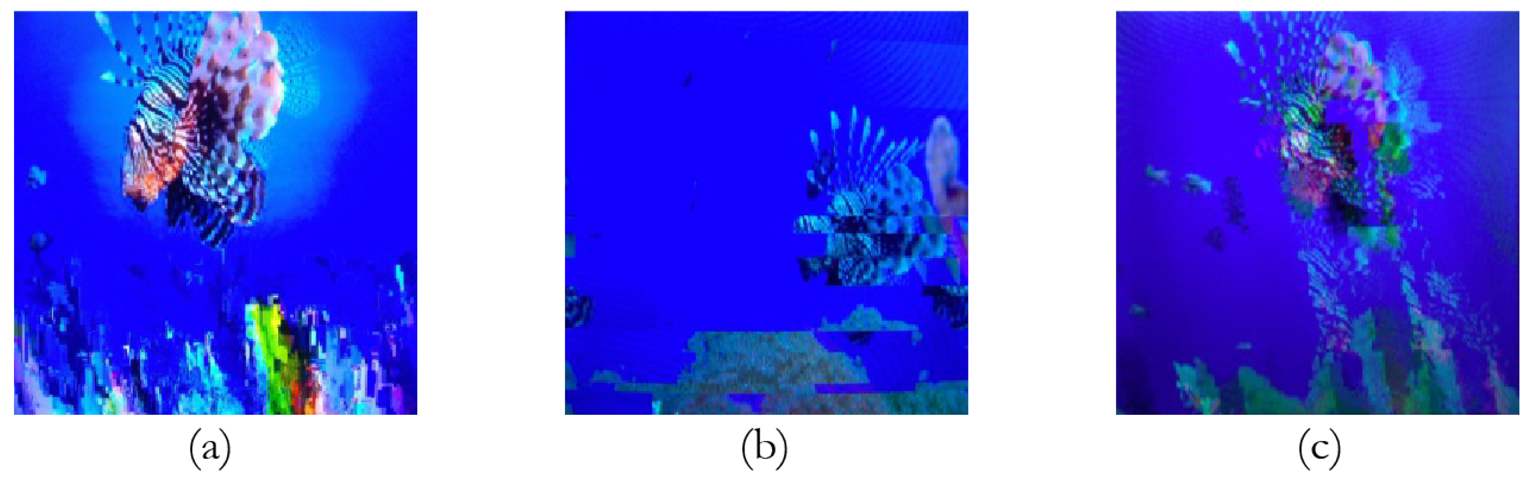
Figure 2 shows a comparison between real mosaic anomalies (
Figure 2a) and those simulated on 60frames (
Figure 2b) and DenserGlitch (
Figure 2c) datasets, respectively.
The same preprocessing steps performed for the previous database were also conducted for this second dataset. An amount of 40 video segments with 10 s was produced. The video segments were balanced, i.e., 20 presented no anomalies in any frames while the remaining 20 presented mosaic in all frames. These videos were recorded while being displayed in the screen of a 43-inch device, allowing the generation of 360 video segments composed of 60 frames obtained with 50% overlap between the frames of subsequent samples. When compared to the 60frames dataset, the mosaic simulation was expected to be more realistic in DenserGlitch. In addition, since the frames were captured by recording the video while it was displayed, even using a camera with the same sample rate as the video’s, some slight oscillations of the frame rates can break the sync in a way that the camera may capture the transition between different frames in the video. This phenomenon may occur in a real scenario. However, this dataset presents two disadvantages: (1) it is significantly smaller than the other two datasets; and (2) all anomalous videos contain defects in every frame, which makes the defect detection problem less challenging.
3.1.3. The_1R
The video capture process for this dataset is similar to the process used to generate the DenserGlitch dataset, including the same camera. Again, two different screen sizes and 10 different camera positions were used per device, providing 78 video segments for each class. The samples were generated using digital image processing before the data capture. Therefore, 60-frame video segments presenting anomalies added as needed were provided, allowing the generation of 3120 samples (1560 per class). The 78 anomalous segments produced for each camera position were equally split into four types of defects. Besides, the amount of defects in a single video was defined according to the following proportions: 46% of the samples contained 1 defect, 31% contained 2 defects, 15% contained 3 defects and 8% contained 4 defects. This proportion was empirically defined based on the observed frequency of each defect in the production line.
To try to prevent possible bias towards some specific type of anomaly, samples with 2 or 3 defects were evenly split for every possible combination of anomalies. The defects’ extension was determined by a normal distribution () truncated in 1. Random values were generated according to this distribution every time a defect was added, independently of its type or the amount of anomalies in a given sample. When adding a defect in a sample, the starting frame of the anomaly was randomly chosen between the positions that could allocate the defect’s full length, as determined by the normal distribution.
The anomalies in this dataset were simulated as follows: mosaics as in DenserGlitch; and freezes and black screens as in the 60frames dataset, except for the fact that all defects were introduced before the videos’ capture. This way, neighbor frames between freezes or black screen are slightly different due to tiny oscillations of the camera or other external factors not controlled during the video capture process. There is also frame loss simulated by skipping some intermediate frames of the videos, producing temporal jumps. During the capture, a colorful screen was used to tag the start and end of each 60-frame segment inside a larger video that was displayed. This strategy allowed the automatic segmentation of the long captured video into a series of shorter instances. Additionally, a camera sample rate oscillations led to unintended events of frame loss in some instances. As a result, the total length of the samples was reduced to 55 frames to enable using most of the generated instances.
3.2. The Proposed 3D-GAN
Six different models were investigated in this paper: a proposed 3D-GAN; a custom 3D-CNN; a spatio-temporal autoencoder; 3D ResNet-34; C3D; and MoViNet-A2. The models 3D ResNet and C3D are considered state-of-the-art methods [
34] while MoViNet-A2 is a computation and memory-efficient network recently proposed to cope with streaming video. Our proposed GAN is detailed in this section and the next section provides a short summary of the baseline.
We proposed a solution using 3D-GAN whose custom generator is designed to generate anomalous videos. The discriminator component, on the other hand, learns only from the normal class data. This way, the proposed method simultaneously generates the anomalous samples and is capable of anomaly detection. Therefore, instead of the traditional fake vs. real adversarial competition, anomalous instances generated from the real ones will be recognized.
When analyzing the results achieved by the classical generator network of a GAN, we observed that the instances generated were not similar enough to real anomalies. Regarding this analysis, we decided to build a custom non-neural network-based generator for providing anomalous videos from the normal ones. This was performed by inserting the anomaly into normal video instances using two groups of transformations: (1) spatial; and (2) temporal. The first group was composed of the following transformations:
Gaussian noise;
Salt-and-pepper noise;
Poisson noise;
Failure in a color channel;
Defective pixels on display;
Jitter;
Digital channel packet loss.
It is important to note that these defects are mainly observed as spatial features. However, since temporal anomalies can occur in the digital channel problem, the generator was also responsible for generating the temporal-based defects below:
Freezing;
Temporal jumps;
Black screen;
Glitch between frames.
All transformations employed by our generator have parameters. For instance, the Gaussian noise depends on two parameters: mean and variance. Taking into account that the mean can be considered zero or simply removed, the variance is the only parameter that controls the noise intensity, i.e., the higher the variance, the higher the severity of the noise. Another example is the black screen transformation, whose parameter is the number of black frames to be inserted into the video. In this case, the number of black frames defines the severity of the anomaly. As explained in the next paragraphs, the transformation parameters are dynamically adjusted according to the loss provided by the discriminator network.
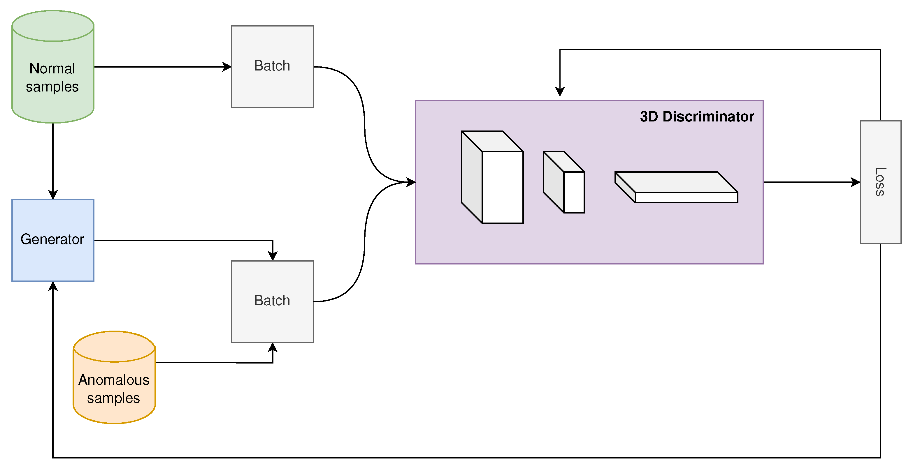
Figure 3 shows the learning process of the model. In each cycle, a batch of normal videos is randomly selected to be fed to the discriminator. The same batch of normal videos is also provided to the generator, which applies temporal and spatial transformations to each normal video in order to generate anomalous instances. The generator provides anomalous videos using the discriminator loss function as an adjustment factor to better generate these instances. Hence, parameters that determine the severity of the anomaly, such as the number of anomalous frames for the black screen transformation and the variance of the Gaussian noise, vary with the discriminator loss. For instance, the variance of the Gaussian noise reduces with the loss of the discriminator. Thus, the better the discriminator, the smoother the generated anomalies will be and the more difficult they will be to detect. For each type of anomaly, upper and lower limits were defined. Therefore, both the anomaly types and their parameters are experimentally adjustable.
In order to extract features only provided by a physical camera as similar as possible to the actual device used in real tests, a small number of real captured anomalous instances (equivalent to 25% of the number of normal instances) was used in our method. When a real anomalous instance was used, a Gaussian smoothing filter was employed before the instance was fed to the discriminator to prevent possible over-adjustments due to the differences between real captured instances and the generated instances. Our preliminary experiments indicated that this process allows the model to achieve better generalization. In addition, based on observations conducted in the assembly line, the generator chooses the group of transformations to be inserted into the normal instances according to the following fixed distribution: 50% for spatial transformations; 30% for temporal transformations; and 20% for real anomalous instances. The transformations from each group are randomly chosen.
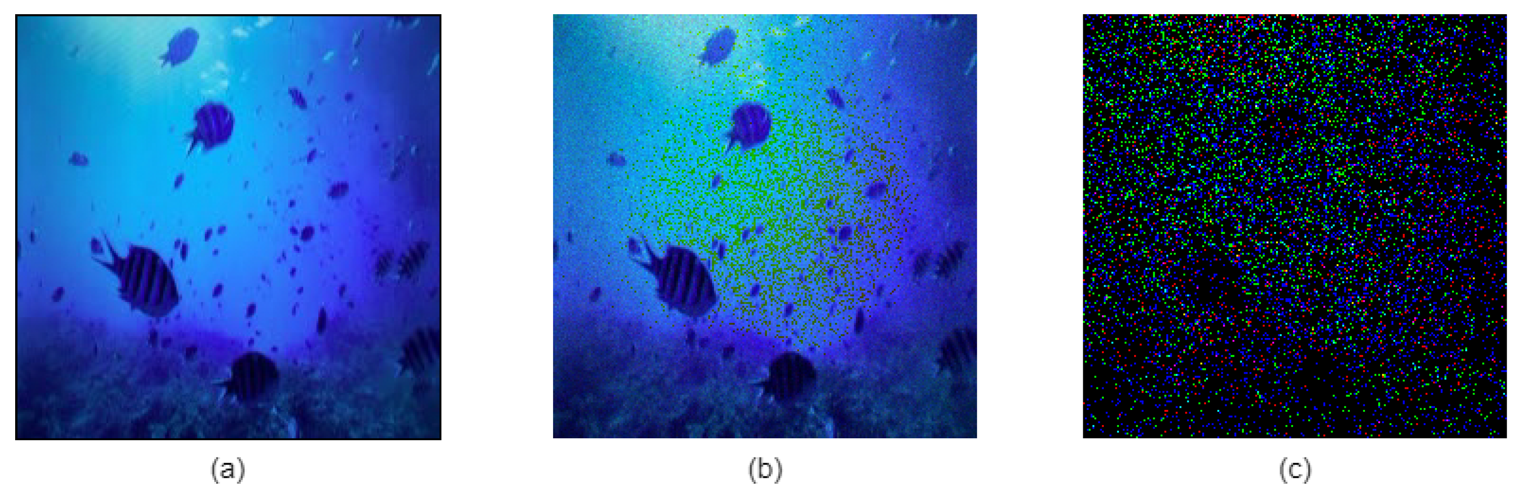
As mentioned before, the artificial generator uses the discriminator loss function as an adjustment factor, generating “more complex” anomalous videos as the discriminator learns.
Figure 4 shows examples of anomalous frames generated by employing the Gaussian transformation to a normal frame. The original normal frame is shown in
Figure 4a. Since the noise severity is defined according to the loss of the discriminator, the anomalous frame in (c) shows high severe noise as a result of the high loss provided by the discriminator, whilst it becomes more realist and smoother as the discriminator loss is reduced.
In terms of the discriminator component,
Table 1 summarizes its architecture. This network is composed of 3 convolutional layers with Leaky ReLU as the activation function, which allows a small and non-zero gradient when the unit is not active. We also added a dropout hidden layer with a 0.3 dropout rate to mitigate overfitting. Due to the possibility that the fully connected layers are prone to overfitting, thus hampering the generalization ability of the overall network [
35], we also applied GlobalMaxPooling3D to take the maximum value of each feature map. This results in a vector being directly fed into the sigmoid layer.
3.3. Baselines
Four supervised approaches were investigated in this paper: (1) a 3D-CNN we customized for the specific-purpose application; and (2) three pre-trained methods: 3D ResNet-34, C3D and MoViNet-A2. The first model was described in the next section and the remaining CNNs are summarized in
Section 3.3.3. Moreover, we also employed a semi-supervised method: an autoencoder described in
Section 3.3.2.
3.3.1. Customized 3D-CNN
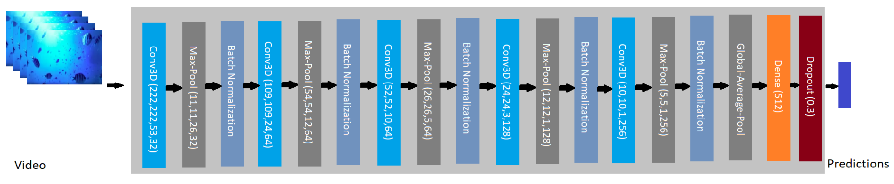
The architecture defined for the 3D-CNN is summarized in
Figure 5. It is composed of 5 3D convolution layers, each followed by a max-pooling and a batch normalization layer. Despite not being clear in the literature whether to use dropout and/or batch normalization to optimize the model focusing on generalization, our experiments pointed out batch normalization layers as a better option. It is worth mentioning that similar results were observed in [
36]. Their results indicate that batch normalization improved model accuracy without considerably increasing the training time. The opposite was observed when using dropout layers, since these incurred a reduction in the model accuracy of evaluating anomalies. These authors concluded that batch normalization layers allowed the model to increase its performance.
The weights were initialized using Glorot Normal Initialization [
37] and the convolution layers employed the rectified linear unit (ReLU) as the activation function. After the last convolutional layer, the global average polling 3D process for temporal data is carried out. In this process, the final normalization of the feature maps is performed to allow each feature map to be converted into a single value. Then, a dense layer is added after the Global Average Polling 3D layer. Finally, dropout is used to focus on reducing overfitting. In addition, since this is a binary problem, the last layer employs sigmoid as the activation function. Therefore, the prediction reaches values close to 1 when an anomaly is detected and close to 0 otherwise. Finally, the remaining hyperparameters applied are: cross entropy and Adam—using a learning rate of
—as the loss function and optimization algorithm, respectively. All hyperparameters were experimentally tuned.
3.3.2. Autoencoder
A semi-supervised learning approach was also investigated in this paper. Precisely, we employed the spatio-temporal residual autoencoder (R-STAE), recently proposed in [
22]. As described in
Section 2.2, this architecture is composed of ConvAE and Conv.LSTM layers, with the addition of residual blocks that result in lower reconstruction errors.
To employ this model using our datasets, the input size was modified to 224 × 224. In addition, Adam with a learning rate of
was the optimizer employed, as was performed for the customized 3D-CNN. The mean squared error (MSE) was used to calculate the average squared difference between the reconstructed and real frames. This method assigns a label to the input instance based on the normality score calculated using the equation below, also employed in [
22].
The normality score values are expected to be higher for normal instances and lower for the anomalous ones. Hence, the score taken from Equation (
1) is compared against an empirically defined threshold.
3.3.3. Pre-Trained 3D-CNN
3D ResNet: The 3D version of ResNet-34 [
19] was chosen as one of the baselines in this paper. The input size, optimizer, and learning rate value were the same as that used in the previous approaches. The network was built with squeeze-and-excitation [
38] layers, which improves the network resources with small computation overhead but without increasing the network depth.
C3D: It is a generic 3D-CNN proposed in [
21] to learn video features by modeling temporal information using pre-trained 3D convolution and 3D pooling operations. It has 8 convolution layers (3D) and 5 pooling layers. The C3D network was originally designed for action recognition; however, it is also very effective in other tasks such as anomaly detection in surveillance videos [
34]. In this work, the same hyperparameters employed for the previous methods were used with this model: input size = 224 × 224; learning rate =
; and Adam as the optimizer.
MoViNet-A2: It is a member of a family of computation- and memory-efficient 3D CNNs (from A0 to A5) recently proposed in [
20]. The three first models (MoViNets A0, A1, and A2) are lightweight methods that can be used on mobile devices. The model employed in this work is the MoviNet-A2, since the input dimension used with the previous baseline models matches its training resolution (224 × 224). Even focusing on a trade-off between efficiency and accuracy, it is expected that MoviNets-A2 achieves lower accuracy when compared to the other supervised CNN investigated in this paper.
4. Experimental Results
Our experiments can be split into two main series. In the first series, all six investigated deep learning models are compared using the three datasets generated in this work. Then, the second series is performed by comparing the same six models on an external dataset. The objective of this second series was to study the behavior of the investigated methods when trained and tested on a related but different dataset. This analysis is especially important to test the generalizability as well as the transferability of the representations learned by the generator component proposed in this paper. First, however, we presented a description of our experimental protocol.
4.1. Experimental Protocol
The three datasets proposed in this paper are described in
Section 3.1. For each dataset, 30% of the samples were reserved as the test partition while the remaining instances were further divided into training and validation partitions with, respectively, 40% and 30% of the total samples. The total amount of examples for each dataset was summarized in
Table 2. The samples’ selection for each partition was not random because subsequent videos of a given camera positioning share frames. Considering the fact that 10 different camera positions were used for each device in each dataset, data from different positions were divided into partitions as follows: samples from three positions from each device for the test set; four different positions for the training set; and the remaining three for the validation set. This guarantees that all instances from a given camera position would always be in the same partition, preventing information leaks from the training data to the testing data. Exploiting this strategy, the experimental results were validated using k-fold validation (
), choosing different sets of camera positions for each data partition.
The external dataset investigated in the second series of experiments was the University of Houston Camera Tampering Detection Dataset (UHCTD) [
39], proposed to test camera tampering detection methods. Tampering corresponds to an unauthorized or an accidental change in the view of a surveillance camera. In the UHCTD dataset, this includes covering, defocusing and intentionally moving cameras with malicious intent such as committing theft or property damage. In our work, the tampering instances are grouped to form the anomalous class.
The dataset consists of 576 instances of tampering induced over 288 h of video captured by two surveillance cameras whose resolutions are 2048 × 1536 and 1280 × 960, respectively. To maintain the same experimental protocol adopted for the other datasets investigated in this work, videos were sampled at 55 frames, with 224 × 224 spatial resolution. However, the data partitioning proposed by the UHCTD authors [
39] was maintained, using the traditional hold-out validation strategy. Hence, after sampling, 30,252 samples of normal videos and 10,572 samples of anomalous videos were obtained to compose the training set. For the test set, 60,437 and 21,140 instances composed the normal and abnormal classes, respectively. In both sets, the class distribution is nearly 3:1, with anomalies comprising the minority class.
4.2. Comparing Deep Learning Approaches
The experiments conducted to compare the six investigated approaches achieved the results summarized in
Table 3. Area under the ROC curve (AUC), accuracy, precision and recall were calculated to determine the performance of the approaches. In addition, the number of processed frames per second (FPS) was also reported to compare the time cost. Values in bold indicate the best result in each dataset.
Although the mosaic simulation in the DenserGlitch dataset was expected to be more realistic, all approaches reached the highest possible performance in this dataset, except for the autoencoder. The justification for this high performance in DenserGlitch when compared to the results reached on the other datasets is that DenserGlitch is less complex in nature, as it presents only one type of anomaly (mosaic) and the anomalous samples present a mosaic in all frames. For the two datasets presenting temporal and spatial defeats, the proposed 3D-GAN achieved a better area under the curve and higher accuracy and recall compared to the supervised methods pre-trained and customized 3D-CNN (cust. 3D-CNN) in the 60frames dataset.
In terms of the 1R dataset, 3D ResNet was superior while 3D-GAN, C3D and cust. 3D-CNN provided equivalent performances. It is interesting to observe the results attained by MoViNet-A2. Despite being a lightweight architecture, we can see in
Table 3 a 12% accuracy reduction in the 1R dataset compared to the best-performing model (3D ResNet). However, in the 60frames dataset we see a much larger accuracy difference. It is important to mention that larger MoViNets (A3–A5) would probably reduce this difference since it has been shown that MoViNet-A5 attains state-of-the-art results in different applications [
20].
These results show that the proposed custom generator module seems to be steadily beneficial for the anomaly detection task using 3D-GAN, since this approach consistently achieved high performance in all datasets, even when only using 25% of labeled anomalous instances, whilst 3D ResNet, C3D, MoViNet and the cust. 3D-CNN were trained using 100% of labeled anomalous instances. This is a very competitive advantage as it avoids the need for a large set of manually labeled anomalous data.
The results achieved by the autoencoder, on the other hand, were significantly worse than those of the other five methods. Despite being expected, since autoencoder is an unsupervised approach, we believe this performance may still be increased by better fine-tuning the appropriate threshold value. While this method is strongly dependent on such a hyperparameter, finding its appropriate value without any validation samples of the anomalous class is very challenging. In addition, this parameter is totally problem dependent.
In terms of time cost, the customized 3D-CNN is most likely the solution establishing the best trade-off between the accuracy and time cost. This method reached the highest FPS in the 60frames and 1R datasets whilst the 3D-GAN was better in the DenserGlith dataset. In contrast, the autoencoder achieved the worst FPS values in all three datasets. The MoViNet-A2 model achieved intermediate FPS values. This is due to the fact that this model is determined by image resolution and FPS values. Therefore, the largest MoViNet models are able to reach higher FPS.
4.3. Generalization Analysis
The first series of experiments has shown that the generator module proposed in this work allowed the 3D-GAN to attain comparable and even better results than the supervised methods, despite only using of the labeled anomalous instances. However, it is not a general-purpose generator. This may constitute a limitation as the generator cannot easily fit a various range of problems. In order to analyze this aspect, in this second series, we conducted experiments using the external dataset UHCTD.
The results shown in
Table 4 indicate an order relation between the CNN-based methods investigated for the UHCTD dataset in terms of performance. C3D reached the highest AUC, accuracy and precision. Then, 3D-ResNet was slightly better than the customized 3D-CNN, except in recall. Finally, MoViNet was 8% worse in AUC when compared to C3D. On the other hand, it provided the highest recall among the CNN-based methods. All supervised methods outperformed the 3D-GAN model, while, again, the autoencoder provided the worst results. As expected, the reason for the significantly degraded performance of the 3D-GAN in UHCTD is probably the problem-dependency of the custom generator. Especially noteworthy is the recall rate obtained using the 3D-GAN model, which was the lowest recall performance among all models investigated. This result indicates how unsuccessful the 3D-GAN was in trying to identify all anomalies. In terms of FPS, the customized 3D-CNN was also the best approach.
However, if the generator is customized, e.g., by providing some modifications in the defects used to generate the anomalous instances, for a specific-purpose application, the final performance will improve. Taking into account the fact that the 3D-GAN method used in this paper is semi-supervised, considering all the available data as normal and the existence of a few anomalous instances to customize and train the generator, the 3D-GAN approach is highly recommended.
5. Conclusions
In this paper, we propose a GAN-based anomaly detection model by using a custom generator component to generate samples of videos presenting spatio-temporal defects. The two components (discriminator and generator) are adversely trained to simultaneously generate anomalies along with learning to perform anomaly detection. The proposed method only requires normal data and few instances of the non-anomalous class in the training process. We applied our method to three datasets with defects of TV digital encoding which were introduced in this paper to simulate real-world industry-oriented failures. Moreover, we investigated the generalizability of representations learned by the proposed generator in an external dataset created to test camera tampering detection methods. Finally, we compared the results to a custom 3D CNN model, an autoencoder model and three pre-trained CNN, precisely C3D, MoViNet and 3D ResNet.
The main results of our experiments successfully demonstrated that the proposed generator helped the 3D-GAN model to achieve a performance compared to the results of the supervised state-of-the-art 3D ResNet and C3D, as well as the lightweight MoViNet, without an increased time cost. However, due to the problem dependency of the proposed custom generator, we observed a significant degraded performance of the 3D-GAN in the external dataset. In the future, we will try to extend our approach to be a more general-purpose method for irregularity detection.


 ,
, 


