Control Performance, Stability Conditions, and Bifurcation Analysis of the Twelve-Pole Active Magnetic Bearings System

Abstract

The active magnetic bearings system plays a vital role in high-speed rotors technology, where many research articles have discussed the nonlinear dynamics of different categories of this system such as the four-pole, six-pole, eight-pole, and sixteen-pole systems. Although the twelve-pole system has many advantages over the eight-pole one (such as a negligible cross-coupling effect, low power consumption, better suspension behaviors, and high dynamic stiffness), the twelve-pole system oscillatory behaviors have not been studied before. Therefore, this article is assigned to explore the effect of the magneto-electro-mechanical nonlinearities on the oscillatory motion of the twelve-pole system controlled via a proportional derivative controller for the first time. The normalized equations of motion that govern the system vibrations are established by means of classical mechanics. Then, the averaging equations are extracted utilizing the asymptotic analysis. The influence of all system parameters on the steady-state oscillation amplitudes is explored. Stability charts in a two-dimensional space are constructed. The stable margin of both the system and control parameters is determined. The obtained investigations reveal that proportional gain plays a dominant role in reshaping the dynamics and motion bifurcation of the twelve-pole systems. In addition, it is found that stability charts of the system can be controlled by simply utilizing both the proportional and derivative gains. Moreover, the numerical simulations showed that the twelve-poles system can exhibit both quasiperiodic and chaotic oscillations besides the periodic motion depending on the control parameters’ magnitude.

1. Introduction

An active magnetic bearings system (AMBS) is a mechanism that supports rotating shafts applying a controllable magnetic force without any physical contact. The working principle of the AMBS is illustrated schematically in Figure 1, where this system consists of six basic elements that are the stator, rotor, electromagnetic poles, proximity sensors, digital controller, and power amplifiers. The stator is the stationary part of the active magnetic bearings on which the electromagnetic poles are fixed. Electromagnetic poles are the element that provides a controllable electromagnetic attractive force to suspend the rotor system within the stator in its hovering position. To make sure the provided force is controllable, the rest of the elements (i.e., the proximity sensors, digital controller, and power amplifiers) are required to form what is known as a closed-loop control system. Simply, the AMBS is works as follows: (1) the proximity sensors measure the instantaneous vibrations $x\left(t\right)$ and $y\left(t\right)$ of the rotor; (2) the measured signals $x\left(t\right)$ and $y\left(t\right)$ are sent to the digital controller to manipulate them according to the provided control algorithm; (3) the manipulated signals (i.e., control signals) are fed back again to the power amplifiers, which in turn apply controlled electrical currents to the electromagnetic poles; and (4) finally, the electromagnetic poles generate a corresponding attractive magnetic force that allows the rotor system to rotate without lateral oscillations in X and Y directions. The frictionless feature of AMBS provides many advantages over the conventional bearings system such as the clean environmental operations of the machines, less maintenance, long working time, and no necessity for lubrication. Accordingly, the huge engineering applications and many advantages of the AMBS have attracted scientists and engineers to design and investigate the dynamical characteristic of the different configurations for such systems. Ji et al. [1] presented analytical investigations for the bifurcation behaviors of the four-pole AMBS. The authors concluded that the four-pole system may suffer from a sensitivity to the initial conditions. In addition, the Hopf, saddle-connection, and saddle-node bifurcations were reported. Saeed et al. [2,3] studied the vibrations control of the six-pole system. They discussed the oscillatory characteristics of the system in both the radial and Cartesian control strategies. They reported that the six-pole system can exhibit small vibration amplitudes and complex bifurcation behavior in the case of Cartesian control. On the other hand, it is found that the six-pole system can exhibit a simple bifurcation behavior such as the Duffing oscillator with strong vibrations in the radial control. The eight-pole AMBS with different configurations and control techniques has been extensively investigated [4,5,6,7,8,9,10,11,12,13,14,15,16,17]. Ji et al. [4,5] and Saeed et al. [6] presented theoretical and numerical investigations for the eight-pole system at the primary and super harmonic resonance conditions. The authors reported the dominance of the nonlinearities and the complexity of the motion bifurcation. The modal oscillations of the eight-pole AMBS was examined by Yang et al. [7]. The system steady-state orbital oscillations were investigated utilizing the asymptotic analysis along with the phase-difference energy-ratio method. The introduced analysis illustrated that the system could perform either quasiperiodic or elliptic motion only. Saeed et al. [8,9] introduced two novel control methods to mitigate the nonlinear vibrations of the eight-pole system at the primary resonance. The first control technique was to couple the rotor system to a second-order filter linearly, while the second control method was to connect the rotor system to a second-order filter in a nonlinear form. Recently, Saeed et al. [10] investigated the influence of the dynamical behaviors of the eight-pole AMBS including the rub-impact force between the rotor and stator. The authors concluded that the eight-pole system may respond with periodic, quasiperiodic, or chaotic motion depending on the magnitude of the impact stiffness coefficient and the value of dynamical friction. The eight-pole rotor system with time varying stiffness coefficient was investigated extensively by Zhang et al. [11,12,13,14,15,16], where Shilnikov multi-pulse chaotic behavior was reported.

The dynamical characteristics and motion bifurcation of the sixteen-pole AMBS system were explored under different control algorithms [17,18,19,20,21,22,23]. Saeed et al. [17,18] introduced a detailed investigation for the sixteen-pole system with constant stiffness coefficients. They studied the influence of Cartesian and radial control methodologies on both the bifurcation characteristics and vibration reduction of the AMBS system. The authors reported that the rotor system has quartic stable periodic motions in the case of Cartesian control, while the system behaves like a Duffing oscillator with a hardening spring characteristic at the radial control case. Zhang and his team introduced a detailed investigation for the sixteen-pole AMBS’ having time-varying stiffness coefficients [19,20,21,22,23]. The capability of the active magnetic bearings system on generating a controllable magnetic attractive force without physical contact with the rotor has attracted scientists and engineers to employ the AMBS with some control algorithms to serve as an adaptive actuator that can be used to reshape the dynamical behaviors of some rotating machinery [24,25,26,27,28,29,30,31,32,33]. Ishida and Inoue [24] proposed a novel nonlinear absorber using four-pole AMBS to suppress the lateral vibration of a nonlinear rotor system. Saeed et al. [25,26,27,28,29,30,31,32] employed the AMBS as an active actuator to control and reshape the oscillatory behaviors of the rotating machines by applying different control techniques. Srinivas et al. [33] introduced an important review study that summarized the huge applications of the rotor active magnetic bearings system.

According to the above discussions, it is noticed that nonlinear dynamical behaviors of the twelve-pole rotor system have not been studied before [34,35,36,37]. However, the twelve-pole system has many advantages over the eight-pole system such as low power consumption, negligible cross-coupling, better suspension behaviors, and high dynamic stiffness [37]. Therefore, this article is dedicated to exploring the dynamical characteristics of the twelve-pole system for the first time. The nonlinear equations of motion that govern the system dynamics in $X$ and $Y$ directions are established, and the corresponding averaging equations are extracted. The effects of the different parameters on the lateral oscillation amplitudes are discussed. The stability charts in a two-dimensional space are established. The stable limits of the system and control parameters are reported. The acquired results illustrated that the twelve-pole system can respond with periodic, quasiperiodic, or chaotic oscillations depending on the system and control parameters. In addition, the obtained stability charts confirmed the possibility of controlling both the motion bifurcation and vibration amplitudes of the studied system using the control gains.

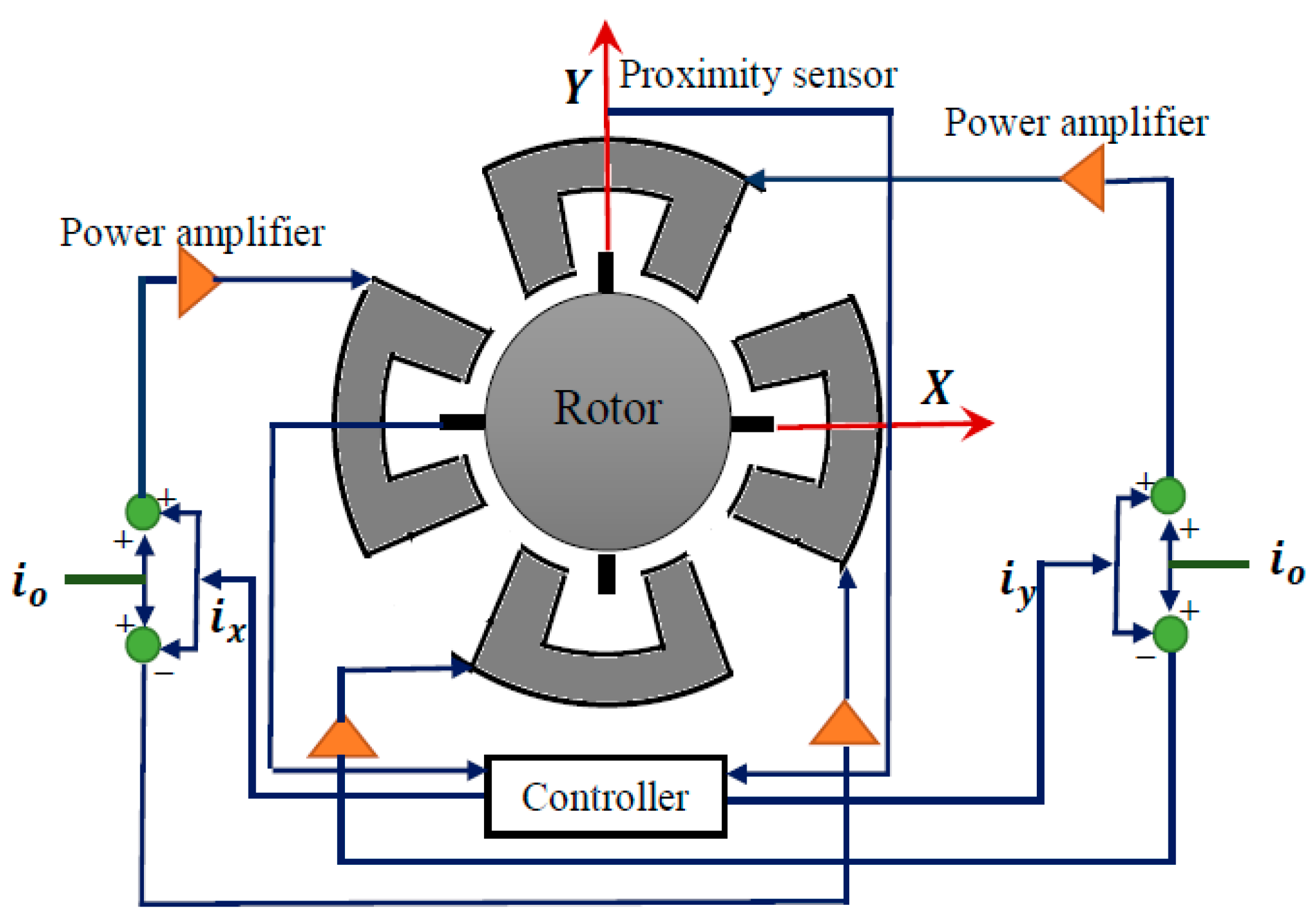
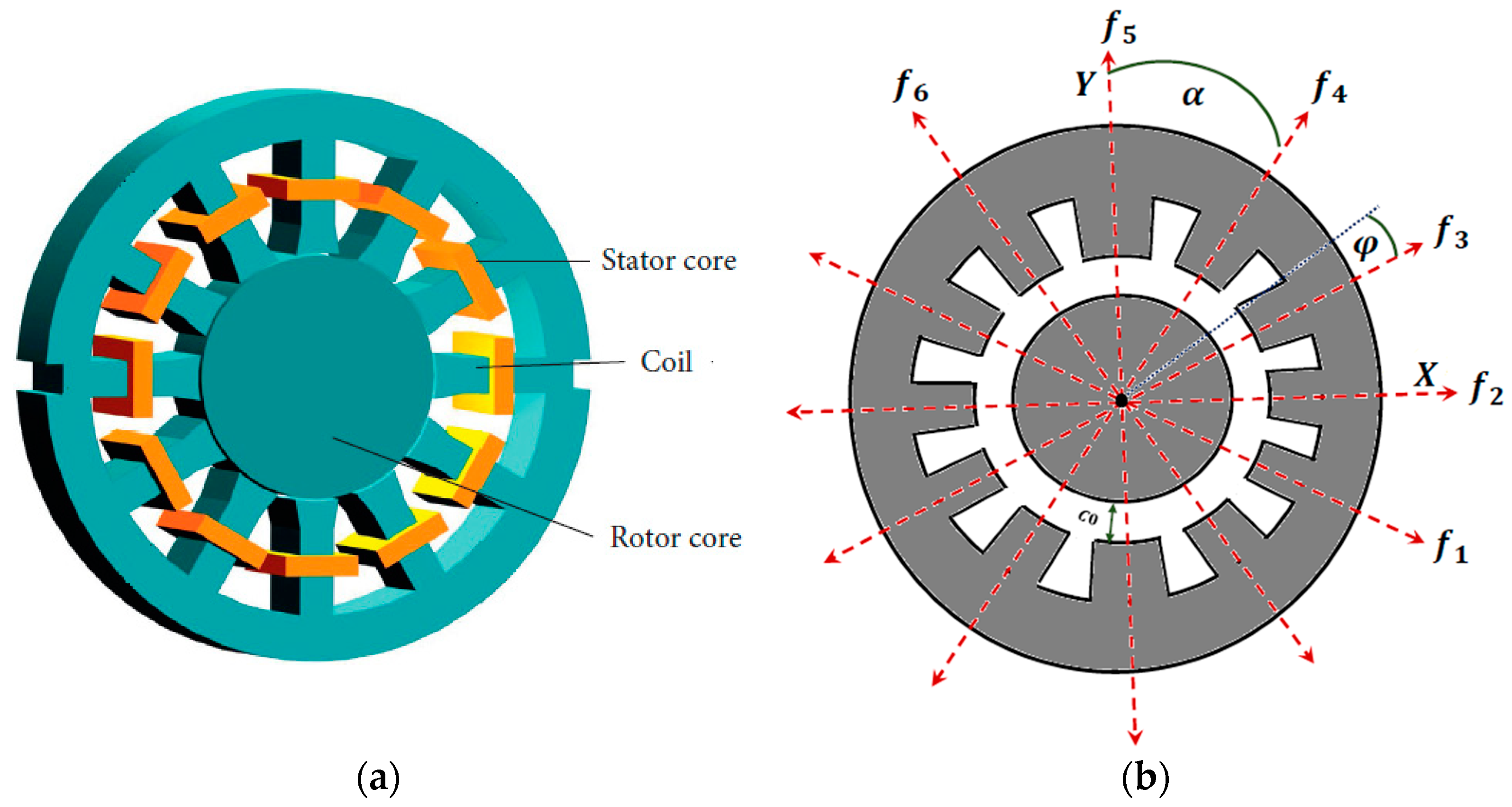
2. Twelve-Pole System Nonlinear Model

Figure 2 depicts a schematic diagram for the twelve-pole rotor system. The rotor is investigated as a two-degree-of-freedom system that oscillates in $X$ and $Y$ directions. The twelve electromagnetic poles are responsible for controlling the system vibrations via generating controllable attractive forces $R_X$ and $R_Y$ in both the horizontal and vertical directions, respectively. Therefore, the differential equations that govern the system motion can be expressed as follows [38,39]:

$$m\ddot{x}(t)=me{\psi }^2\cos (\psi t)+R_X$$

(1)

$$m\ddot{y}(t)=me{\psi }^{2}sin(\psi t)+R_Y$$

(2)

where $m$ is the rotor mass, $\frac{d^{2}x}{d{t}^2}=\ddot{x}\left(t\right)$ and $\frac{d^{2}y}{d{t}^2}=\ddot{y}\left(t\right)$ are the horizontal and vertical accelerations of the rotor system, $e$ is the eccentricity of the rotating disc, $\psi$ is the disc angular speed, and $R_X$ and $R_Y$ are the net attractive forces of the twelve poles in $X$- and $Y$-direction. By considering the symmetric design of the twelve-pole system, the attractive force of each opposite pair of the poles $(f_j,j=1,2,\dots ,6$) can be expressed as follows [39]:

$$f_j=\frac{{\mu }_0{N}^{2}A\cos (\phi )}{4}\left[\frac{{\left(I_0-I_j\right)}^2}{{\left(c_0-{\delta }_j\right)}^2}-\frac{{\left(I_0+I_j\right)}^2}{{\left(c_0+{\delta }_j\right)}^2}\right],j=1\cdots 6$$

(3)

where ${\mu }_0$ is the free space permeability, $N$ the number of turns of each coil for the twelve poles, $A$ is the cross-sectional area of each pole, $I_0$ is the permanentized electrical current, $I_j$ is the control current in the $j$th pole, $c_0$ is the nominal air gap size as shown in Figure 2b, ($c_0-{\delta }_j$) is the instantaneous air gap of the $j$th pole.

Accordingly, for the small displacements $x$ and $y$ of the rotor system, ${\delta }_j$ can be expressed as follows:

$$\begin{array}{lll}{\delta }_1=x\cos (\alpha )-y\sin (\alpha ),& {\delta }_2=x,& {\delta }_3=x\cos (\alpha )+y\sin (\alpha )\\ {\delta }_4=x\sin (\alpha )+y\cos (\alpha ),& {\delta }_5=y,& {\delta }_6=-x\sin (\alpha )+y\cos (\alpha )\end{array}\}$$

(4)

where, $\alpha ={30}^{\mathrm{o}}$ is the angle between every successive two poles (See Figure 2b). The control currents $I_j$ are designed such that the forces $f_1,f_2,$ and $f_3$ are proportional to the displacement $x\left(t\right)$ and velocity $\dot{x}\left(t\right)$, while $f_4,f_5,$ and $f_6$ are proportional to the displacement $y\left(t\right)$ and velocity $\dot{y}\left(t\right)$. Therefore, the control currents are designed as follows:

$$I_1=I_2=I_3=k_{1}x+k_2\dot{x},I_4=I_5=I_6=k_{1}y+k_2\dot{y}$$

(5)

where $k_1$ is known as proportional gain, while $k_2$ represents the derivative gain. Now, by substituting Equations (4) and (5) into Equation (3), and then expanding the resulting equations up to the third order using Maclaurin series, we can obtain the forces $f_i,\left(i=1,2,\dots ,8\right)$ as given in Appendix A. Accordingly, the net attractive forces $R_X$ and $R_Y$ of the twelve-pole system in the horizontal and vertical directions can be expressed as follows:

$$R_X=f_2+(f_1+f_3)\cos (\alpha )+(f_4-f_6)\sin (\alpha )$$

(6)

$$R_Y=f_5+(f_4+f_6)\cos (\alpha )+(f_3-f_1)\sin (\alpha )$$

(7)

Substituting Equations (6) and (7) into Equations (1) and (2), and then replacing the original variables and parameters with the following dimensionless variables and parameters: $x^{*}=\frac{x}{c_0},y^{*}=\frac{y}{c_0},$ $t^{*}=\zeta t,{\dot{x}}^{*}=\dot{\frac{x}{\zeta c_0}},$ ${\dot{y}}^{*}=\dot{\frac{y}{\zeta c_0}},{\ddot{x}}^{*}=\frac{\ddot{x}}{{\zeta }^2{c}_0},{\ddot{y}}^{*}=\frac{\ddot{y}}{{\zeta }^2{c}_0},p=\frac{c_0}{I_0}{k}_1,d=\frac{c_0\zeta }{I_0}{k}_2,f=\frac{e}{c_0},\Omega =\frac{\omega }{\zeta }$, $\zeta =\sqrt{4{\mu }_0{I}_0^2{N}^{2}Acos\left(\phi \right)/m{c}_0^3}$, with omitting the asterisks for simplicity, we have

$$\begin{array}{l}\ddot{x}+2\mu \dot{x}+{\omega }^{2}x-({\alpha }_1{x}^3+{\alpha }_{2}x{y}^2+{\alpha }_3{x}^2\dot{x}+{\alpha }_4\dot{x}{y}^2+{\alpha }_{5}x{y}^2+{\alpha }_{6}x{\dot{x}}^2\\ +{\alpha }_{7}xy\dot{y})={\Omega }^{2}f\cos (\Omega t)\end{array}$$

(8)

$$\begin{array}{l}\ddot{y}+2\mu \dot{y}+{\omega }^{2}y-({\alpha }_1{y}^3+{\alpha }_{2}y{x}^2+{\alpha }_3{y}^2\dot{y}+{\alpha }_4\dot{y}{x}^2+{\alpha }_{5}y{\dot{x}}^2+{\alpha }_{6}y{\dot{y}}^2\\ +{\alpha }_{7}yx\dot{x})={\Omega }^{2}f\sin (\Omega t)\end{array}$$

(9)

The normalized nonlinear dynamical system that is given by Equations (8) and (9) describes the relative oscillations ($x$ and $y$) of the twelve-pole system in $X$ and $Y$ directions with respect to the nominal air gap size $c_0$, where the dimensionless coefficients $\mu ,\omega ,{\alpha }_j$ ($j=1,2,\dots ,7$) are given in Appendix B. To investigate the performance of the proposed control method, bifurcations behaviors, and stability conditions of the twelve-pole system, asymptotic analysis is employed to obtain the autonomous amplitude-phase equations and the corresponding nonlinear algebraic system of Equations (8) and (9) as given in the following section.

3. Analytical Investigation and Autonomous Amplitude-Phase Equations

This section is dedicated to obtaining an analytical solution for the twelve-pole system. Accordingly, the first-order approximate solution for Equations (8) and (9) can be sought utilizing the multiple-time scale perturbation procedures as follows [40]:

$$x(t,\epsilon )=x_0(T_0,T_1)+\epsilon x_1(T_0,T_1)$$

(10)

$$y(t,\epsilon )=y_0(T_0,T_1)+\epsilon y_1(T_0,T_1)$$

(11)

where $\epsilon$ is an artificial parameter used as a book-keeping parameter only, $T_0=t$ and $T_1=\epsilon t$ represent the fast and slow time scales, respectively. So, the ordinary derivatives $\frac{d}{dt}$ and $\frac{d^2}{d{t}^2}$ can be written using the chain rule for derivatives as:

$$\frac{d}{dt}=D_0+\epsilon D_1,\frac{d^2}{d{t}^2}=D_0^2+2\epsilon D_0{D}_1,D_j=\frac{\partial }{\partial T_j},j=0,1$$

(12)

Depending on the system nonlinearities, the coefficients of Equations (8) and (9) should be scaled as follows to execute the multiple time scales procedure:

$$\mu =\epsilon \widehat{\mu },{\alpha }_j=\epsilon {\widehat{\alpha }}_j,f=\epsilon \widehat{f},j=1,\dots ,7$$

(13)

Now, by inserting Equations (10)–(12) into Equations (8) and (9), and equating the coefficients that have the same power of $\epsilon$, we get

$$O\left({\epsilon }^0\right):$$

$$\left(D_0^2+{\omega }^2\right)x_0=0$$

(14)

$$\left(D_0^2+{\omega }^2\right)y_0=0$$

(15)

$$O\left({\epsilon }^1\right)\text{:}$$

$$\begin{array}{cc}\hfill \left(D_0^2+{\omega }^2\right)x_1& =-2D_0{D}_1{x}_0-2\widehat{\mu }{D}_0{x}_0+{\widehat{\alpha }}_1{x}_0^3+{\widehat{\alpha }}_2{x}_0{y}_0^2+{\widehat{\alpha }}_3{x}_0^2{D}_0{x}_0\hfill \\ & +{\widehat{\alpha }}_4{y}_0^2{D}_0{x}_0+{\widehat{\alpha }}_5{x}_0{(D_0{y}_0)}^2+{\widehat{\alpha }}_6{x}_0{(D_0{x}_0)}^2+{\widehat{\alpha }}_7{x}_0{y}_0{D}_0{y}_0\hfill \\ & +\widehat{f}{\Omega }^2\cos (\Omega T_0)\hfill \end{array}$$

(16)

$$\begin{array}{cc}\hfill \left(D_0^2+{\omega }^2\right)y_1& =-2D_0{D}_1{y}_0-2\widehat{\mu }{D}_0{y}_0+{\widehat{\alpha }}_1{y}_0^3+{\widehat{\alpha }}_2{y}_0{x}_0^2+{\widehat{\alpha }}_3{y}_0^2{D}_0{y}_0\hfill \\ & +{\widehat{\alpha }}_4{x}_0^2{D}_0{y}_0+{\widehat{\alpha }}_5{y}_0{(D_0{x}_0)}^2+{\widehat{\alpha }}_6{y}_0{(D_0{y}_0)}^2+{\widehat{\alpha }}_7{y}_0{x}_0{D}_0{x}_0\hfill \\ & +\widehat{f}{\Omega }^2\sin (\Omega T_0)\hfill \end{array}$$

(17)

The solutions of homogeneous differential equations given by Equations (14) and (15) are:

$$x_0(T_0,T_1)=A(T_1)e^{i\omega T_0}+\overline{A}(T_1)e^{-i\omega T_0}$$

(18)

$$y_0(T_0,T_1)=B(T_1)e^{i\omega T_0}+\overline{B}(T_1)e^{-i\omega T_0}$$

(19)

where $A\left(T_1\right)$ and $B\left(T_1\right)$ are two unknowns that will be determined in the subsequent steps of analysis, and $\overline{A}\left(T_1\right)$ and $\overline{B}\left(T_1\right)$ are the conjugate functions of the unknowns $A\left(T_1\right)$ and $B\left(T_1\right)$. By inserting Equations (18) and (19) into Equations (16) and (17), yields

$$\begin{array}{cc}\hfill \left(D_0^2+{\omega }^2\right)x_1& =[-2i\omega (D_{1}A)-2i\widehat{\mu }\omega A+3{\widehat{\alpha }}_1{A}^2\overline{A}+2{\widehat{\alpha }}_{2}AB\overline{B}+{\widehat{\alpha }}_2\overline{A}{B}^2+i{\widehat{\alpha }}_3\omega A^2\overline{A}+2i{\widehat{\alpha }}_4\omega AB\overline{B}\hfill \\ & -i{\widehat{\alpha }}_4\omega \overline{A}{B}^2+2{\widehat{\alpha }}_5{\omega }^{2}AB\overline{B}-{\widehat{\alpha }}_5{\omega }^2\overline{A}{B}^2+{\widehat{\alpha }}_6{\omega }^2{A}^2\overline{A}+i{\widehat{\alpha }}_7\omega \overline{A}{B}^2]e^{i\omega T_0}+[{\widehat{\alpha }}_1{A}^3\hfill \\ & +{\widehat{\alpha }}_{2}A{B}^2+i{\widehat{\alpha }}_3\omega A^3+i{\widehat{\alpha }}_4\omega A{B}^2-{\widehat{\alpha }}_5{\omega }^{2}A{B}^2-{\widehat{\alpha }}_6{\omega }^2{A}^3+i{\widehat{\alpha }}_7\omega A{B}^2]e^{3i\omega T_0}\hfill \\ & +\frac{1}{2}{\Omega }^2\widehat{f}{e}^{i\Omega T_0}\hfill \end{array}$$

(20)

$$\begin{array}{cc}\hfill \left(D_0^2+{\omega }^2\right)y_1& =[-2i\omega (D_{1}B)-2i\widehat{\mu }\omega B+3{\widehat{\alpha }}_1{B}^2\overline{B}+2{\widehat{\alpha }}_{2}BA\overline{A}+{\widehat{\alpha }}_2\overline{B}{A}^2+i{\widehat{\alpha }}_3\omega B^2\overline{B}+2i{\widehat{\alpha }}_4\omega BA\overline{A}\hfill \\ & -i{\widehat{\alpha }}_4\omega \overline{B}{A}^2+2{\widehat{\alpha }}_5{\omega }^{2}BA\overline{A}-{\widehat{\alpha }}_5{\omega }^2\overline{B}{A}^2+{\widehat{\alpha }}_6{\omega }^2{B}^2\overline{B}+i{\widehat{\alpha }}_7\omega \overline{B}{A}^2]e^{i\omega T_0}+[{\widehat{\alpha }}_1{B}^3\hfill \\ & +{\widehat{\alpha }}_{2}B{A}^2+i{\widehat{\alpha }}_3\omega B^3+i{\widehat{\alpha }}_4\omega B{A}^2-{\widehat{\alpha }}_5{\omega }^{2}B{A}^2-{\widehat{\alpha }}_6{\omega }^2{B}^3+i{\widehat{\alpha }}_7\omega B{A}^2]e^{3i\omega T_0}\hfill \\ & -\frac{1}{2}i{\Omega }^2\widehat{f}{e}^{i\Omega T_0}\hfill \end{array}$$

(21)

To obtain a bounded solution for Equations (20) and (21), the possible resonant conditions should be determined first, which are the primary (i.e., $\Omega =\omega$) and subharmonic (i.e., $\Omega =3\omega$) resonance cases. Accordingly, to investigate the system dynamics at primary response condition, the detuning parameter $\sigma$ is introduced to distinguish the closeness of the rotor angular speed to the twelve-pole system natural frequency as follows:

$$\Omega =\omega +\sigma =\omega +\epsilon \widehat{\sigma }$$

(22)

By introducing Equation (22) into Equations (20) and (21), we get

$$\begin{array}{cc}\hfill \left(D_0^2+{\omega }^2\right)x_1& =[-2i\omega (D_{1}A)-2i\widehat{\mu }\omega A+3{\widehat{\alpha }}_1{A}^2\overline{A}+2{\widehat{\alpha }}_{2}AB\overline{B}+{\widehat{\alpha }}_2\overline{A}{B}^2+i{\widehat{\alpha }}_3\omega A^2\overline{A}\hfill \\ & +2i{\widehat{\alpha }}_4\omega AB\overline{B}-i{\widehat{\alpha }}_4\omega \overline{A}{B}^2+2{\widehat{\alpha }}_5{\omega }^{2}AB\overline{B}-{\widehat{\alpha }}_5{\omega }^2\overline{A}{B}^2+{\widehat{\alpha }}_6{\omega }^2{A}^2\overline{A}+i{\widehat{\alpha }}_7\omega \overline{A}{B}^2\hfill \\ & +\frac{1}{2}{(\omega +\sigma )}^2\widehat{f}{e}^{i\epsilon \widehat{\sigma }{T}_0}]e^{i\omega T_0}+[{\widehat{\alpha }}_1{A}^3+{\widehat{\alpha }}_{2}A{B}^2+i{\widehat{\alpha }}_3\omega A^3+i{\widehat{\alpha }}_4\omega A{B}^2-{\widehat{\alpha }}_5{\omega }^{2}A{B}^2\hfill \\ & -{\widehat{\alpha }}_6{\omega }^2{A}^3+i{\widehat{\alpha }}_7\omega A{B}^2]e^{3i\omega T_0}\hfill \end{array}$$

(23)

$$\begin{array}{cc}\hfill \left(D_0^2+{\omega }^2\right)y_1& =[-2i\omega (D_{1}B)-2i\mu \omega B+3{\widehat{\alpha }}_1{B}^2\overline{B}+2{\widehat{\alpha }}_{2}BA\overline{A}+{\widehat{\alpha }}_2\overline{B}{A}^2+i{\widehat{\alpha }}_3\omega B^2\overline{B}\hfill \\ & +2i{\widehat{\alpha }}_4\omega BA\overline{A}-i{\widehat{\alpha }}_4\omega \overline{B}{A}^2+2{\widehat{\alpha }}_5{\omega }^{2}BA\overline{A}-{\widehat{\alpha }}_5{\omega }^2\overline{B}{A}^2+{\widehat{\alpha }}_6{\omega }^2{B}^2\overline{B}+i{\widehat{\alpha }}_7\omega \overline{B}{A}^2\hfill \\ & -\frac{1}{2}i{(\omega +\sigma )}^2\widehat{f}{e}^{i\epsilon \widehat{\sigma }{T}_0}]e^{i\omega T_0}+[{\widehat{\alpha }}_1{B}^3+{\widehat{\alpha }}_{2}B{A}^2+i{\widehat{\alpha }}_3\omega B^3+i{\widehat{\alpha }}_4\omega B{A}^2-{\widehat{\alpha }}_5{\omega }^{2}B{A}^2\hfill \\ & -{\widehat{\alpha }}_6{\omega }^2{B}^3+i{\widehat{\alpha }}_7\omega B{A}^2]e^{3i\omega T_0}\hfill \end{array}$$

(24)

To have a bounded solution for Equations (23) and (24), the coefficients of $e^{i\omega T_0}$ should vanish. So, the solvability conditions of Equations (23) and (24) are:

$$\begin{array}{l}-2i\omega (D_{1}A)-2i\widehat{\mu }\omega A+3{\widehat{\alpha }}_1{A}^2\overline{A}+2{\widehat{\alpha }}_{2}AB\overline{B}+{\widehat{\alpha }}_2\overline{A}{B}^2+i{\widehat{\alpha }}_3\omega A^2\overline{A}+2i{\widehat{\alpha }}_4\omega AB\overline{B}-i{\widehat{\alpha }}_4\omega \overline{A}{B}^2\\ +2{\widehat{\alpha }}_5{\omega }^{2}AB\overline{B}-{\widehat{\alpha }}_5{\omega }^2\overline{A}{B}^2+{\widehat{\alpha }}_6{\omega }^2{A}^2\overline{A}+i{\widehat{\alpha }}_7\omega \overline{A}{B}^2+\frac{1}{2}{(\omega +\sigma )}^2\widehat{f}{e}^{i\widehat{\sigma }{T}_1}=0\end{array}$$

(25)

$$\begin{array}{l}-2i\omega (D_{1}B)-2i\widehat{\mu }\omega B+3{\widehat{\alpha }}_1{B}^2\overline{B}+2{\widehat{\alpha }}_{2}BA\overline{A}+{\widehat{\alpha }}_2\overline{B}{A}^2+i{\widehat{\alpha }}_3\omega B^2\overline{B}+2i{\widehat{\alpha }}_4\omega BA\overline{A}-i{\widehat{\alpha }}_4\omega \overline{B}{A}^2\\ +2{\widehat{\alpha }}_5{\omega }^{2}BA\overline{A}-{\widehat{\alpha }}_5{\omega }^2\overline{B}{A}^2+{\widehat{\alpha }}_6{\omega }^2{B}^2\overline{B}+i{\widehat{\alpha }}_7\omega \overline{B}{A}^2-\frac{1}{2}i{(\omega +\sigma )}^2\widehat{f}{e}^{i\widehat{\sigma }{T}_1}=0\end{array}$$

(26)

To investigate Equations (25) and (26), the unknown functions $A\left(T_1\right)$ and $B\left(T_1\right)$ can be expressed in the polar form such that [40]:

$$A(T_1)=\frac{1}{2}a(T_1)e^{i{\theta }_1(T_1)},B(T_1)=\frac{1}{2}b(T_1)e^{i{\theta }_2(T_1)}$$

(27)

Inserting Equation (27) into Equations (25) and (26) and reverting to the original system parameters (i.e., $t=\frac{T_1}{\epsilon },\widehat{\sigma }=\frac{\sigma }{\epsilon }.\widehat{\mu }=\frac{\mu }{\epsilon },\widehat{f}=\frac{f}{\epsilon },{\widehat{\alpha }}_j=\frac{{\alpha }_j}{\epsilon },j=1,\dots .,7$), and then separating the real and imaginary parts of the resulting equations, we can obtain the following autonomous system of the first-order nonlinear differential equations:

$$\begin{array}{ll}\frac{da}{dt}=F_1(a,b,{\phi }_1,{\phi }_2)=& -\mu a+\frac{1}{8}({\alpha }_3)a^3+\frac{1}{4}{\alpha }_{4}a{b}^2+\frac{1}{8}(-{\alpha }_4+{\alpha }_7)a{b}^2\cos (2{\phi }_2-2{\phi }_1)\\ & -\frac{1}{8}(\frac{{\alpha }_2}{\omega }-{\alpha }_5\omega )a{b}^2\sin (2{\phi }_2-2{\phi }_1)+\frac{1}{2\omega }{(\omega +\sigma )}^{2}f\sin {\phi }_1\end{array}$$

(28)

$$\begin{array}{ll}\frac{db}{dt}=F_2(a,b,{\phi }_1,{\phi }_2)=& -\mu b+\frac{1}{8}({\alpha }_3)b^3+\frac{1}{4}{\alpha }_{4}b{a}^2+\frac{1}{8}(-{\alpha }_4+{\alpha }_7)b{a}^2\cos (2{\phi }_2-2{\phi }_1)\\ & +\frac{1}{8}(\frac{{\alpha }_2}{\omega }-{\alpha }_5\omega )b{a}^2\sin (2{\phi }_2-2{\phi }_1)-\frac{1}{2\omega }{(\omega +\sigma )}^{2}f\cos {\phi }_2\end{array}$$

(29)

$$\begin{array}{ll}\frac{d{\phi }_1}{dt}=F_3(a,b,{\phi }_1,{\phi }_2)=& \sigma +\frac{1}{8}(\frac{3{\alpha }_1}{\omega }+{\alpha }_6\omega )a^2+\frac{1}{4}(\frac{{\alpha }_2}{\omega }+{\alpha }_5\omega )b^2+\frac{1}{8}(\frac{{\alpha }_2}{\omega }-{\alpha }_5\omega )b^2\cos (2{\phi }_2-2{\phi }_1)\\ & +\frac{1}{8}(-{\alpha }_4+{\alpha }_7)b^2\sin (2{\phi }_2-2{\phi }_1)+\frac{1}{2a\omega }{(\omega +\sigma )}^{2}f\cos {\phi }_1\end{array}$$

(30)

$$\begin{array}{ll}\frac{d{\phi }_2}{dt}=F_4(a,b,{\phi }_1,{\phi }_2)=& \sigma +\frac{1}{8}(\frac{3{\alpha }_1}{\omega }+{\alpha }_6\omega )b^2+\frac{1}{4}(\frac{{\alpha }_2}{\omega }+{\alpha }_5\omega )a^2+\frac{1}{8}(\frac{{\alpha }_2}{\omega }-{\alpha }_5\omega )a^2\cos (2{\phi }_2-2{\phi }_1)\\ & -\frac{1}{8}(-{\alpha }_4+{\alpha }_7)a^2\sin (2{\phi }_2-2{\phi }_1)+\frac{1}{2b\omega }{(\omega +\sigma )}^{2}f\sin {\phi }_2\end{array}$$

(31)

where ${\phi }_1=\sigma t-{\theta }_1,{\phi }_2=\sigma t-{\theta }_2$. Now, by substituting Equation (27) into Equations (18) and (19), and then inserting the resulting equations into Equations (10) and (11), yields

$$x(t)=a(t)\cos \left(\Omega t-{\phi }_1(t)\right)$$

(32)

$$y(t)=b(t)\cos \left(\Omega t-{\phi }_2(t)\right)$$

(33)

Accordingly, Equations (32) and (33) represent the periodic solution of the twelve-pole system given by Equations (8) and (9), where the amplitudes ($a\left(t\right)$ and $b\left(t\right))$ and the corresponding phase angles (${\varphi }_1\left(t\right)$ and ${\varphi }_2\left(t\right))$ are functions of time that evolve depending on the nonlinear dynamical system given by Equations (28)–(31). Therefore, at the steady-state periodic vibrations of the twelve-pole system, we have $\frac{da}{dt}=\frac{db}{dt}=\frac{d{\phi }_1}{dt}=\frac{d{\phi }_2}{dt}=0$. Substituting $\frac{da}{dt}=\frac{db}{dt}=\frac{d{\phi }_1}{dt}=\frac{d{\phi }_2}{dt}=0$ into Equations (28)–(31), we can obtain the following nonlinear coupled algebraic equations:

$$\begin{array}{l}-\mu a+\frac{1}{8}({\alpha }_3)a^3+\frac{1}{4}{\alpha }_{4}a{b}^2+\frac{1}{8}(-{\alpha }_4+{\alpha }_7)a{b}^2\cos (2{\phi }_2-2{\phi }_1)-\frac{1}{8}(\frac{{\alpha }_2}{\omega }-{\alpha }_5\omega )a{b}^2\sin (2{\phi }_2-2{\phi }_1)\\ +\frac{1}{2\omega }{(\omega +\sigma )}^{2}f\sin {\phi }_1=0\end{array}$$

(34)

$$\begin{array}{l}-\mu b+\frac{1}{8}({\alpha }_3)b^3+\frac{1}{4}{\alpha }_{4}b{a}^2+\frac{1}{8}(-{\alpha }_4+{\alpha }_7)b{a}^2\cos (2{\phi }_2-2{\phi }_1)+\frac{1}{8}(\frac{{\alpha }_2}{\omega }-{\alpha }_5\omega )b{a}^2\sin (2{\phi }_2-2{\phi }_1)\\ -\frac{1}{2\omega }{(\omega +\sigma )}^{2}f\cos {\phi }_2=0\end{array}$$

(35)

$$\begin{array}{l}\sigma +\frac{1}{8}(\frac{3{\alpha }_1}{\omega }+{\alpha }_6\omega )a^2+\frac{1}{4}(\frac{{\alpha }_2}{\omega }+{\alpha }_5\omega )b^2+\frac{1}{8}(\frac{{\alpha }_2}{\omega }-{\alpha }_5\omega )b^2\cos (2{\phi }_2-2{\phi }_1)+\frac{1}{8}(-{\alpha }_4+{\alpha }_7)b^2\\ \times \sin (2{\phi }_2-2{\phi }_1)+\frac{1}{2a\omega }{(\omega +\sigma )}^{2}f\cos {\phi }_1=0\end{array}$$

(36)

$$\begin{array}{l}\sigma +\frac{1}{8}(\frac{3{\alpha }_1}{\omega }+{\alpha }_6\omega )b^2+\frac{1}{4}(\frac{{\alpha }_2}{\omega }+{\alpha }_5\omega )a^2+\frac{1}{8}(\frac{{\alpha }_2}{\omega }-{\alpha }_5\omega )a^2\cos (2{\phi }_2-2{\phi }_1)-\frac{1}{8}(-{\alpha }_4+{\alpha }_7)a^2\\ \times \sin (2{\phi }_2-2{\phi }_1)+\frac{1}{2b\omega }{(\omega +\sigma )}^{2}f\sin {\phi }_2=0\end{array}$$

(37)

The above nonlinear algebraic system governs both the steady-state vibration amplitudes ($a$ and $b)$ and the phase angles (${\varphi }_1$ and ${\varphi }_2)$ of the twelve-pole system in terms of the rotor eccentricity ($f$), the angular speed ($\sigma =\Omega -\omega$, and the control gains ($p$ and $d$). So, by solving Equations (34)–(37) simultaneously using one of the petameters (i.e., $\sigma ,f,p,d$) as a bifurcation parameter, we can obtain the different response curves as in Figure 3 and Figure 4, etc. In addition, the solution stability of Equations (34)–(37) can be checked via using the Jacobian matrix of the corresponding dynamical system given by Equations (28)–(31). To check the solution stability of Equations (34)–(37), let the solution of Equations (34)–(37) is ($a_0,b_0,{\phi }_{10},{\phi }_{20}$) and assume ($a_1,b_1,{\phi }_{11},{\phi }_{21}$) is a small deviation from this solution. Accordingly, we can write

$$a=a_0+a_1,b=b_0+b_1,{\phi }_1={\phi }_{10}+{\phi }_{11},{\phi }_2={\phi }_{20}+{\phi }_{21}$$

(38)

By differentiating Equation (38), we have

$$\frac{da}{dt}=\frac{d{a}_1}{dt},\frac{db}{dt}=\frac{d{b}_1}{dt},\frac{d{\phi }_1}{dt}=\frac{d{\phi }_{11}}{dt},\frac{d{\phi }_2}{dt}=\frac{d{\phi }_{21}}{dt}$$

(39)

Substituting Equations (38) and (39) into Equations (28)–(31) and expanding for the small deviations $a_1,b_1,{\phi }_{11},$ and ${\phi }_{21}$ keeping the linear terms only, we have

$$\left(\begin{array}{c}\frac{d{a}_1}{dt}\\ \frac{d{b}_1}{dt}\\ \frac{d{\phi }_{11}}{dt}\\ \frac{d{\phi }_{21}}{dt}\end{array}\right)=\left(\begin{array}{cccc}\frac{\partial F_1}{\partial a_1}& \frac{\partial F_1}{\partial b_1}& \frac{\partial F_1}{\partial {\phi }_{11}}& \frac{\partial F_1}{\partial {\phi }_{21}}\\ \frac{\partial F_2}{\partial a_1}& \frac{\partial F_2}{\partial b_1}& \frac{\partial F_2}{\partial {\phi }_{11}}& \frac{\partial F_2}{\partial {\phi }_{21}}\\ \frac{\partial F_3}{\partial a_1}& \frac{\partial F_3}{\partial b_1}& \frac{\partial F_3}{\partial {\phi }_{11}}& \frac{\partial F_3}{\partial {\phi }_{21}}\\ \frac{\partial F_4}{\partial a_1}& \frac{\partial F_4}{\partial b_1}& \frac{\partial F_4}{\partial {\phi }_{11}}& \frac{\partial F_4}{\partial {\phi }_{21}}\end{array}\right)\left(\begin{array}{c}{a}_1\\ b_1\\ {\phi }_{11}\\ {\phi }_{21}\end{array}\right)$$

(40)

The coefficients of the Jacobian matrix are given below in Appendix C. According to the Hartman–Grobman theorem, the linear system given by Equation (40) is topologically equivalent to the nonlinear system given by Equations (28)–(31). Therefore, the solution stability of Equations (34)–(37) can be explored via the eigenvalues of the Jacobian matrix.

4. Bifurcation Analysis, Stability Charts, and Control Performance

Depending on the mathematical modeling and analysis given above, the bifurcation behaviors, stability conditions, and control performance of the twelve-pole rotor system are discussed in this section. The steady-state vibration amplitudes ($a$ and $b$) of the twelve-pole rotor are plotted versus the different parameters by solving the derived nonlinear algebraic Equations (34)–(37). In addition, the stability of these amplitudes is studied via the exploration of the eigen values of Equation (40). In all response curves (i.e., Figures 3–6, 12–14, 19–21 and 25), the solid lines represent the stable solution, and the dotted lines refer to the unstable solutions. As Equations (34)–(37) govern the steady-state oscillation amplitudes of the rotor system that is governed by Equations (8) and (9), numerical simulations for the plotted response curves are performed by solving Equations (8) and (9) using the Runge–Kutta algorithm. The steady-stated oscillation amplitudes that were obtained numerically by solving Equations (8) and (9) are plotted as small-circles (when sweeping the bifurcation parameter forward) and as big-dots (when sweeping the bifurcation parameter backward). The analytical and numerical results are obtained by adopting the following values of the system parameters unless otherwise is mentioned: $p=1.22,d=0.005,\alpha ={30}^{\mathrm{o}},$ $f=0.01$, and $\Omega =\omega +\sigma ,\sigma =0$ [2,3,4,5,6,7,8,9,10].

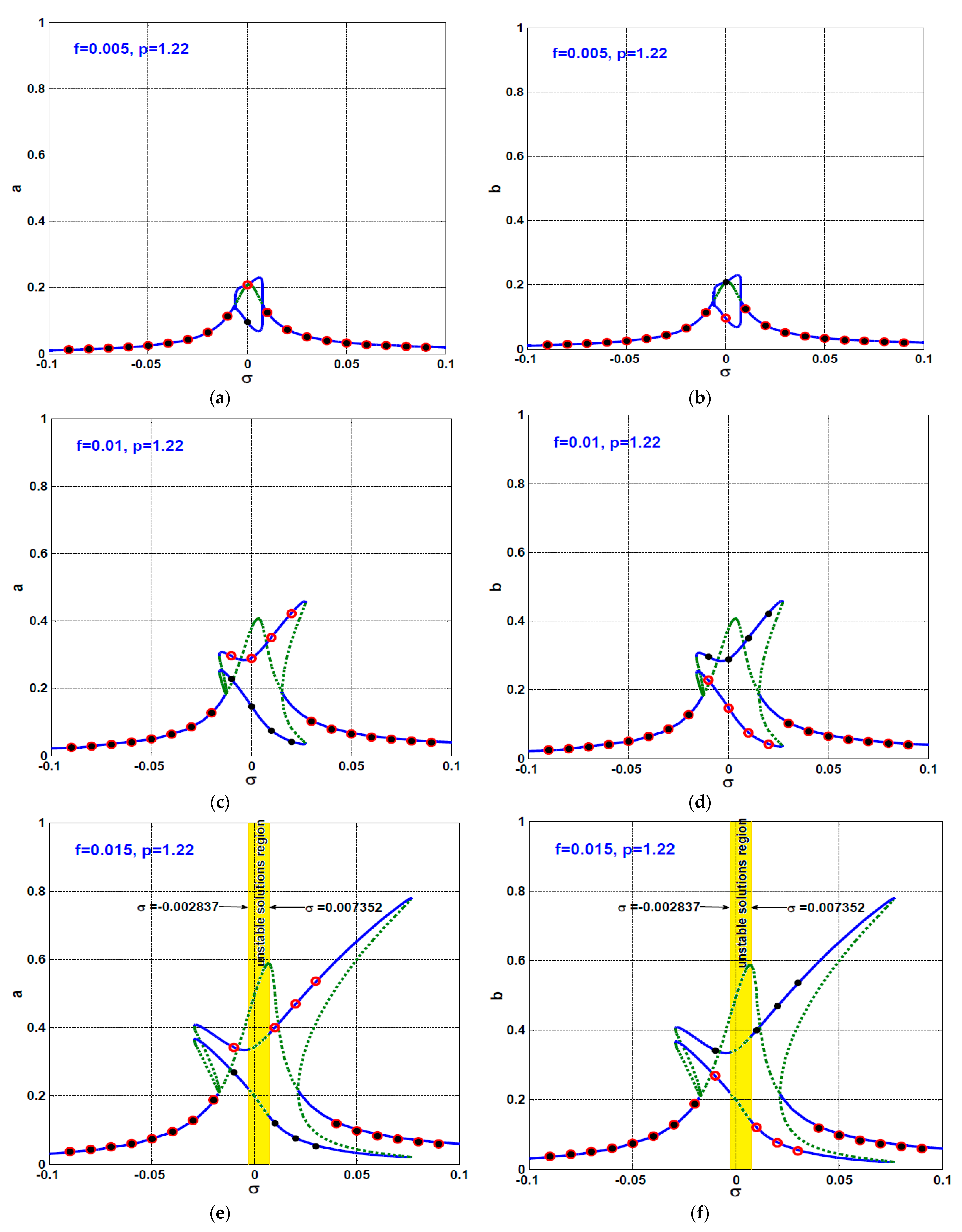
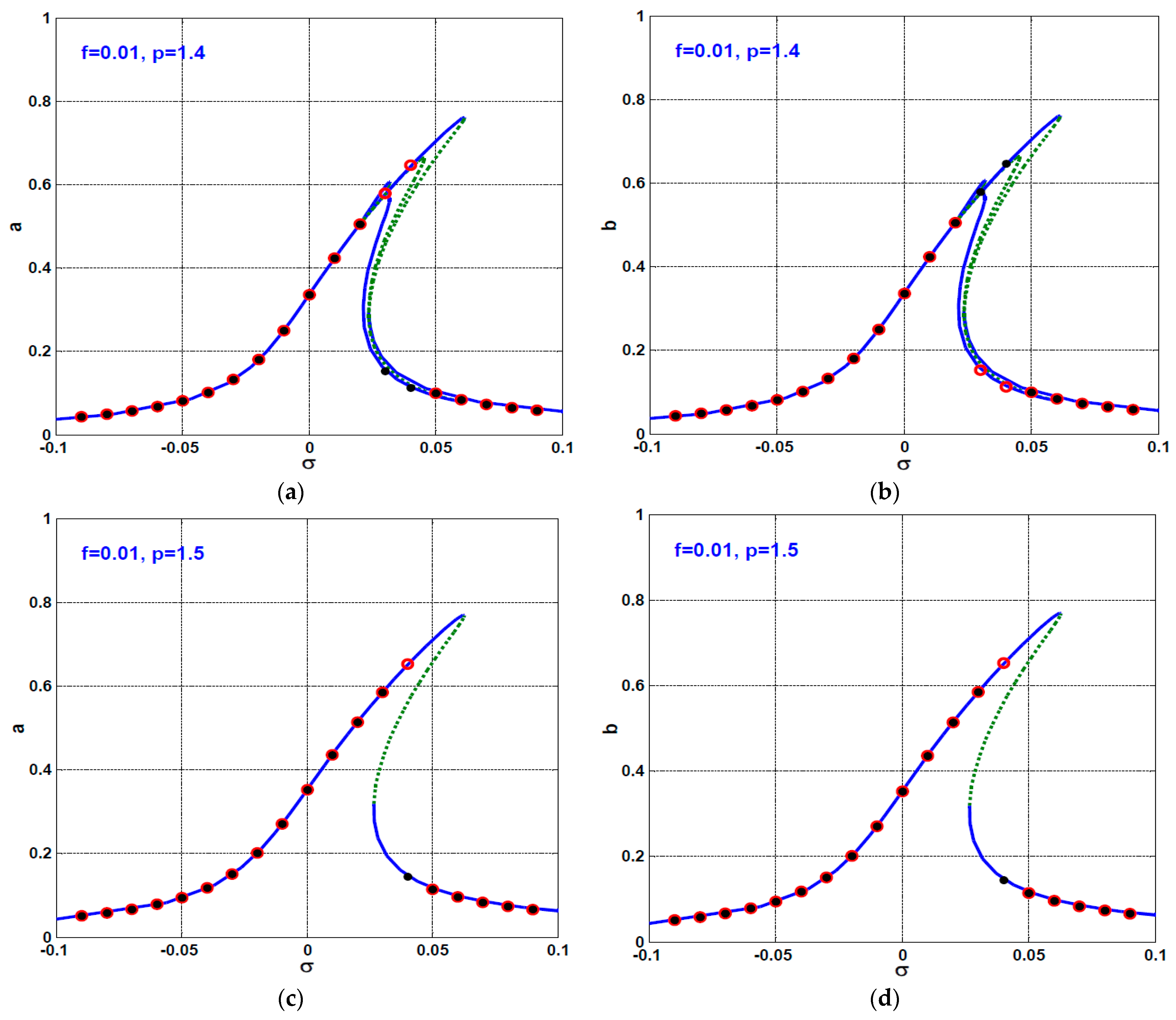
4.1. Influence of the Proportional Gain ($p$) on the Rotor System Dynamics

Before proceeding further, we should remember that the normalized system parameters are defined such that $p=\frac{c_0}{I_0}{k}_1,d=\frac{c_0\zeta }{I_0}{k}_2,$ and $f=\frac{e}{c_0}$. Accordingly, it is easy to deduce that the dimensionless coefficients $p$ and $d$ represent the dimensionless form of the proportional and derivative gains, respectively, while $f$ represents the eccentricity of the rotating disc. In addition, the detuning parameter $\sigma$ denotes the closeness of the system angular speed $\Omega$ to its natural frequency $\omega$ (i.e., $\Omega =\omega +\sigma$). In the following, the stability conditions, bifurcation analysis, and control performance of the twelve-pole system are investigated in terms of the parameters $p,d,f,$ and $\sigma$. Figure 3 illustrates the angular speed response curves of the twelve-pole system at various values of the eccentricity (i.e., $f=0.005,0.01,0.015$) when the proportional gain $p=1.22$. In general, the figure shows that the twelve-pole system has a complicated response near the perfect resonance (i.e., when $\Omega \to \omega$), where the rotor system may possess two and/or three stable periodic solutions besides the unstable one at the same angular speed. In addition, the figure confirms that the vibration amplitudes of the twelve-pole system are monotonic increasing function the eccentricity $f$. Moreover, Figure 3e,f illustrate that the twelve-poles system can lose its stability at a specific angular speed interval (i.e., $-0.002837<\sigma <0.007352$) if $f$ exceeds a specific critical value (i.e., $f=0.015$).

The twelve-pole dynamics at different values of the proportional gain is explored through Figure 4, where Figure 4a,b show the system steady-state vibrations against $\sigma$ at $p=1.4$, while Figure 4c,d depict the system steady-state vibrations against $\sigma$ at $p=1.5$ when fixing the eccentricity at $f=0.01$. Comparing Figure 3c,d with Figure 4c,d, we can notice two important phenomena. The first phenomenon (positive phenomenon) is that the system dynamical behaviors became simpler when increasing $p=1.22$ as in Figure 3c,d to $p=1.5$ as in Figure 4c,d, where the system exhibits a response similar to a Duffing oscillator with hard spring characteristics. The second phenomenon (negative phenomenon) is that the vibration amplitudes ($a\&b$) at $p=1.5$ are about twice the oscillation amplitudes when $p=1.22$.

The sensitivity of the twelve-pole system to the different magnitudes of the rotor eccentricity (i.e., $f=0.005,0.01,$ and $0.015$) when the proportional gain kept fixed at $p=1.5$ is illustrated in Figure 5. The figure shows that the system vibration amplitudes ($a$ and $b$) are a monotonic increasing function of the eccentricity. In addition, the system behaves as a Duffing oscillator with hard spring characteristics in both the horizontal and vertical directions, where the system may have bistable periodic solutions at a specific range of angular speeds. Comparing Figure 3 and Figure 5, it is noticed that the twelve-pole system may lose its stability to respond with aperiodic oscillations when $\Omega \cong \omega$ (i.e., when $\sigma =0.0$) if the eccentricity $f=0.015$ and the proportional gain $p=1.22$ (see Figure 3e,f), meanwhile increasing the proportional gain from $p=1.22$ to $p=1.5$, eliminates the instability conditions as shown in Figure 5.

Due to the dominant role of the proportional gain ($p$) in reshaping the vibration characteristics of the twelve-pole system as demonstrated in Figure 3, Figure 4 and Figure 5, the proportional gain has been employed as a bifurcation parameter where $p$ is plotted versus the vibration amplitudes ($a\&b$) of the twelve-pole system when $f=0.01$ and $\sigma =0.0$ as shown in Figure 6. Clear from the figure is the great influence of the proportional gain on the oscillation amplitudes and bifurcation of the system motion, where the figure shows that the twelve-pole system has no solution as long as the proportional gain $p<1.098$. In addition, the figure depicts that the periodic solution of the twelve-pole system may lose its stability if the gain $p$ exceeds a specific limit (i.e., when $p>1.778$). Moreover, Figure 6 demonstrates that the system may respond with a unique periodic solution or bistable periodic solutions depending on the $p$ magnitude within the interval $1.098<p<1.778$. It is simple to explain the absence of the solution for the twelve-pole system from the engineering point of view when $p<1.098$. By coming back to the definition of the system natural frequency $\omega =\sqrt{2pcos\left(\alpha \right)+p-3}$, where $\omega$ depends only on the proportional gain because $\alpha$ is constant (i.e., $\alpha ={30}^{\mathrm{o}}$ see Figure 3). Accordingly, the selection of the proportional gain in a way that makes ${\omega }^2<0$ (i.e., $p\le 1.098$) is not acceptable from the engineering standpoint, where the system has no solution if its natural frequency is an imaginary value.

To obtain the stability boundaries of proportional control gain in more general form, the stability charts for the twelve-pole system are obtained in both $p-\sigma ,$ and $p-f$ planes, as in Figure 7. The figure illustrates that the system has no solution as long $p<1.098$ regardless of the values of $\sigma$ and $f$, as demonstrated in Figure 7a,b, respectively, where the absence of the solution depends on the magnitude of $p$ and hence the magnitude of the natural frequency $\omega$ as explained above.

To investigate the accuracy of the obtained stability charts shown in Figure 7, a numerical simulation for the twelve-pole system (i.e., solving Equations (8) and (9) using MATLAB ODE45) according to four points $p_1,p_2,p_3$, and $p_4$ that are shown in Figure 7a and are introduced in Figure 8, Figure 9, Figure 10, Figure 11. It is clear that the point $p_1$ is located within the stable solution region. Accordingly, it is expected that the twelve-pole rotor to respond with stable periodic oscillation when tuning the system parameters such that $p=1.8,\sigma =-0.01,f=0.01,$ and $d=0.005$. Figure 8 shows the temporal dynamics of the twelve-pole system according to the point $p_1$ (i.e., $p=1.8,\sigma =-0.01,f=0.01,$ and $d=0.005$), where Figure 8a,b show the instantaneous oscillations of the system, and Figure 8c illustrates the steady-state periodic orbit. In addition, both the corresponding Poincaré-map and frequency spectrum for the system temporal oscillations is constructed, as shown in Figure 8d–g. In general, Figure 8 confirms the stable periodic motion for the studied system at $p=1.8,\sigma =-0.01,f=0.01,$ and $d=0.005$, where the orbital motion, the Poincaré-map, and the frequency spectrum demonstrate that the temporal oscillations contain a single frequency component.

Figure 9 simulates the temporal vibrations of the twelve-pole system according to the point $p_2$ (i.e., $p=1.8,\sigma =0.0,f=0.01,$ and $d=0.005$) that marked in Figure 7a within the unstable solutions region. Figure 9a,b illustrate the instantaneous oscillations of the system, while Figure 9c shows the corresponding unstable periodic orbit. Figure 9a–c show that the twelve-pole system exhibits unstable periodic oscillations when simulated according to the point $p_2$ that agrees accurately with the obtained stability chart is given in Figure 7a. Moreover, to identify the nature of the system motion shown in Figure 9a,b, the corresponding Poincaré-map and frequency spectrum are established as shown in Figure 9d–g. Figure 9d–g depict that the rotor system performs a quasi-periodic oscillation where the Poincaré-map is obtained as a closed curve. In addition, the frequency spectrum shows that the temporal oscillations contain irrational frequency components.

Figure 10 and Figure 11 simulate the twelve-pole system oscillations according to the points $p_3$ and $p_4$ that are marked in Figure 7a, respectively. Figure 10 shows that the rotor system has a quasiperiodic motion when simulated according to the point $p_3$ (i.e., when $p=2.0,\sigma =0.0,f=0.01,$ and $=0.005$) that lies with the unstable solutions region. On the other hand, the system responds with stable periodic motion when simulated according to the point $p_4$ (i.e., when $p=2.0,\sigma =0.01,f=0.01,$ and $=0.005$) that lies with the stable solutions region as shown in Figure 11. Depending on the obtained analytical and numerical results investigations given in Figure 7, Figure 8, Figure 9, Figure 10 and Figure 11, we can confirm the accuracy of the obtained analytical solution that given by Equations (34)–(37) in describing the steady-state motion of the twelve-pole system governed by Equations (8) and (9).

4.2. Influence of the Derivative Gain ($d$) on the Rotor System Dynamics

The influence of the second control parameter (i.e., the derivative gain $d$) on the dynamical behaviors of the twelve-pole system is discussed through Figure 12, Figure 13, Figure 14, Figure 15, Figure 16, Figure 17 and Figure 18. In Figure 12, the twelve-pole system steady-state oscillation amplitudes are plotted against the detuning parameter $\sigma$ at various values of the derivative gain (i.e., when $d=0.005,0.01,$ and $0.015$) when fixing the eccentricity and the proportional gain constant so that $f=0.015$ and $p=1.22$. Comparing Figure 12a,b with Figure 12c,d, it is noticed that the increase in $d$ from $0.005$ to $0.01$ eliminates the unstable motions of the twelve-pole system that appeared in Figure 12a,b and reduces the vibration amplitudes $\left(a\&b\right)$ of the rotor system. However, Figure 12c,d show that the system has a bistable solution near the perfect resonance (i.e., when $\Omega \to \omega$), and the nonlinearity characteristics still dominate the rotor response. However, when increasing the derivative gain from $d=0.01$ to $d=0.015$, as depicted in Figure 12e,f, it forces the twelve-pole system to respond linearly where the bifurcations of the motions are suppressed.

The effect of the derivative gain on the steady-state oscillation amplitudes of the rotor system when fixing $p=1.5$ and $f=0.015$ has been illustrated in Figure 13. It is clear from the figure that the oscillation amplitudes are a monotonic decreasing function of the derivative gain $d$, where the system may respond linearly, and the motion bifurcations disappear at $d=0.015$.

The mechanism of the derivative gain $d$ in eliminating the motion bifurcations and reducing the system vibration amplitudes can be explained based on the definition of the twelve-pole system linear damping coefficient $\mu =\left(cos\left(\alpha \right)+\frac{1}{2}\right)d$. The linear damping coefficient $\mu$ is a constant multiple of the derivative control gain $d$. Therefore, the increase in $d$ is a direct increase of $\mu$, which in turn decreases the oscillation amplitudes and eliminates the bifurcation of the system motion at a specific critical value. Accordingly, the derivative gain is employed as a bifurcation parameter as shown in Figure 14, where the oscillation amplitudes are plotted against $d$ at various values of the proportional gain $p$ (i.e., $p=1.22$ and $p=1.5$) when fixing $f=0.01$ and $\sigma =0.0$. Comparing Figure 14a,b with Figure 14c,d, we can deduce that the amplitudes ($a\&b$) are a monotonic decreasing function of the derivative gain. In addition, the figures show that the system has a complex bifurcation behavior at $p=1.22$, while increasing the proportional gain to $p=1.5$ can eliminate the bifurcation of the system motion. Moreover, Figure 14 shows that the twelve-pole system may lose its stability if $d<0.00435$ when fixing $p=1.22$, while increasing $p$ to became $1.5$ enhances the stability margin (i.e., the system loses its stability if $d<0.0005$ when $p=1.5$).

Accordingly, to investigate the stability boundaries of the derivative control gain as a function of either the rotor eccentricity $f$ or the detuning parameter $d$, the stability chart of the twelve-pole system is established in both $d-\sigma$ plane and $d-f$ plane, as illustrated in Figure 15. It is clear from Figure 15a that the system may lose its stability at a small derivative gain (i.e., $d<0.0045$) if the rotor angular speed $\Omega$ is closed to or equal the natural frequency $\omega$ (i.e., when $\sigma \to 0$). However, increasing the derivative control gain in a way so that $d>0.0045$, guarantees the stability of the twelve-pole system oscillation regardless of the rotor angular speed. Figure 15b shows the stability margin of the derivative gain as a function of the eccentricity $f$. The figure illustrates that the increase in derivative gain makes the twelve-pole system withstand the large eccentricities without losing its stability.

To validate the accuracy of the obtained stability charts shown in Figure 15, a numerical simulation for the rotor system according to the three marked points (i.e., the points $p_1,p_2$ and $p_3$) in Figure 15b is performed, as shown in Figure 16, Figure 17 and Figure 18. Figure 16 simulates the temporal oscillations of the rotor system according to the point $p_1$ (i.e., $d=0.004,f=0.01,p=1.22,$ and $\sigma =0.0$) that is marked in Figure 15b within the unstable solutions region. Figure 16a,b shows the instantaneous vibrations of the twelve-pole system in $X$ and $Y$ directions, while Figure 16c shows the corresponding steady-state orbital motion. In addition, the Poincaré-map and frequency spectrum are shown in Figure 16d–g. Figure 16a–c confirm that the system performs unstable periodic motion when simulated according to the point $p_1$ that agrees with the stability chart given in Figure 15b. Moreover, Figure 16d–g demonstrate that the rotor system performs a quasiperiodic motion. The numerical simulations of the rotor temporal oscillations according to the points $p_2$ and $p_3$ shown in Figure 15b have been illustrated in Figure 17 and Figure 18, respectively. Now, by comparing Figure 16, Figure 17 and Figure 18 with the three marked points ($p_1,p_2$ and $p_3$) shown in Figure 15b, we can confirm the accurate correspondence among the obtained stability chart and the numerical simulations.

Finally, the bifurcation behaviors of the twelve-pole system when utilizing the eccentricity $f$ as the bifurcation control parameter is discussed through Figure 19, Figure 20 and Figure 21, where Figure 19a,b shows the system amplitudes ($a\&b$) versus the rotor eccentricity $f$ when $\sigma =0.0$ at various values of the proportional gain $p$ (i.e., when $p=1.22$ and $p=1.5$). It is clear from Figure 19a,b that the twelve-pole system exhibits complex bifurcations behavior at $p=1.22$. In addition, the figure confirms that the system loses its stability at acritical values of the eccentricity. However, the same Figures (Figure 19a,b) illustrate that the rotor system has a unique stable solution along the $f$ axis when fixing the proportional control gain to be $p=1.5$. Accordingly, we can conclude that the twelve-pole system is robust against instability when subjected to large eccentricities when setting $p=1.5$. Depending on Figure 19a,b, the system bifurcation diagrams are established, as shown in Figure 19c,d, utilizing $f$ as the bifurcation parameter when $p=1.22$ and $p=1.5$. The bifurcation diagrams in Figure 19c,d are obtained via plotting the Poincaré-map of Equations (8) and (9) versus the eccentricity $f$ with a step-size $\mathsf{\Delta }f={10}^{-4}$ and zero initial conditions. Comparing Figure 19a,b with Figure 19c,d, we can confirm the excellent corresponding between the analytic (i.e., Figure 19a,b) and numerical (i.e., Figure 19c,d) results. Figure 20 and Figure 21 are a repetition for Figure 19, but when $\sigma =-0.025$ and $\sigma =0.025$, respectively. By examining Figure 19, Figure 20 and Figure 21 carefully, we can notice three important phenomena. The first one is that the detuning parameter $\sigma$ has a great influence on the critical value of the eccentricity at which the system may lose its stability when $p=1.22$. The second phenomenon is that the twelve-pole system is stable along the $f$ axis regardless of the magnitudes of $\sigma$ if the proportional gain $p=1.5$. The third phenomenon is that the steady-state oscillation amplitudes when $p=1.5$ are greater than the steady-state oscillation amplitudes at $p=1.22$ along the stable interval of the $f$ axis.

As the detuning parameter $\sigma$ has a great influence on the critical value of the eccentricity at which the system may lose its stability as depicted in Figure 19, Figure 20 and Figure 21, the stability chart of the twelve-pole system has been constructed in the $f-\sigma$ plane, as shown in Figure 22a,b, when $p=1.22$ and $p=1.5$, respectively. It is clear from Figure 22a that the twelve-pole system may lose its stability at small eccentricity values when $\sigma =0.0$. However, increasing or decreasing $\sigma$ beyond zero increases the stability margin of the system. On the other hand, the stability chart in Figure 22b depicted that the system is stable for all values of the eccentricity regardless of the detuning parameter magnitude when setting $p=1.5$. Comparing Figure 19, Figure 20 and Figure 21 with Figure 22, we can deduce that Figure 22 is a full picture for Figure 19, Figure 20 and Figure 21 regarding the stability boundaries of $f$ at the different values of $\sigma$ either when $p=1.22$ or $p=1.5$.

Numerical confirmation for the stability charts shown in Figure 22, according to the marked points $p_1$ and $p_2$, is illustrated in Figure 23 and Figure 24 by solving Equations (8) and (9) using MATLAB ode45. Figure 23 illustrates the twelve-pole system temporal oscillations according to the point $p_1$ (i.e., $f=0.05,\sigma =0.0,p=1.22,d=0.005$) that is marked in Figure 22a within the unstable solutions region. Figure 23d–g depict that the twelve-pole rotor performs chaotic motion as the Poincare map and frequency spectrum illustrated, which agrees with the stability chart in Figure 22a. In addition, Figure 24 simulates the twelve-pole system temporal oscillation and the corresponding orbital motion according to the point $p_2$ (i.e., $f=0.05,\sigma =0.0,p=1.5,d=0.005$) that is marked in Figure 22b within the stable solutions region. It is noticed that the rotor system exhibits stable periodic oscillation that is agreed with the stability chart in Figure 22b.

5. Comparison between the System Dynamics at $p=1.22$ and $p=1.5$

Within this section, the efficiency of the proposed controller in both reducing the oscillation amplitudes and stabilizing the system motions is compared when the proportional gain $p=1.22$ and $p=1.5$. Figure 25a,b shows the steady-state vibration amplitudes at $f=0.01$, while Figure 25c,d depicts the steady-state vibration amplitudes at $f=0.015$. It is noticed from Figure 25a,b that the twelve-pole system vibration amplitudes at $p=1.22$ are always smaller than the oscillation amplitudes when $p=1.5$ along the $\sigma$ axis. However, one of the drawbacks of the small proportional gain (i.e., when $p=1.22$) is the complex bifurcation of the system motion. On the other hand, the figures show simple bifurcation behaviors at $p=1.5$, but the system may suffer from high oscillation amplitudes.

Additionally, Figure 25c,d shows the vibration characteristics of the system when $f=0.015$ at $p=1.22$ and $p=1.5$. The figure demonstrates the control system has vibration mitigation efficiency at $p=1.22$ higher than that $p=1.5$. However, the system may lose its stability at the large eccentricities at $p=1.22$. Therefore, the optimal design of the control variables ($p$ and $d$) is a compromising process that depends on the magnitudes of the system parameters (i.e., the eccentricity and angular speed), and the control objectives.

6. Conclusions

The twelve-pole AMBS system vibrational behaviors are extensively analyzed within this article. The classical mechanics principle is applied to derive the system’s equations of motion. Then, the derived mathematical model is solved analytically by utilizing the perturbation analysis to obtain the amplitude-phase modulating equations. Based on the extracted amplitude-phase equations, the steady-state oscillations are explored in terms of all system parameters. The stability charts are established in two-parameter space to investigate the stability margin of the different system parameters. In addition, the obtained results are validated numerically via plotting the system temporal oscillations, orbital motion, Poincaré-map, frequency spectrum, and the bifurcation diagram. According to the presented study, we can conclude with the following important remarks:

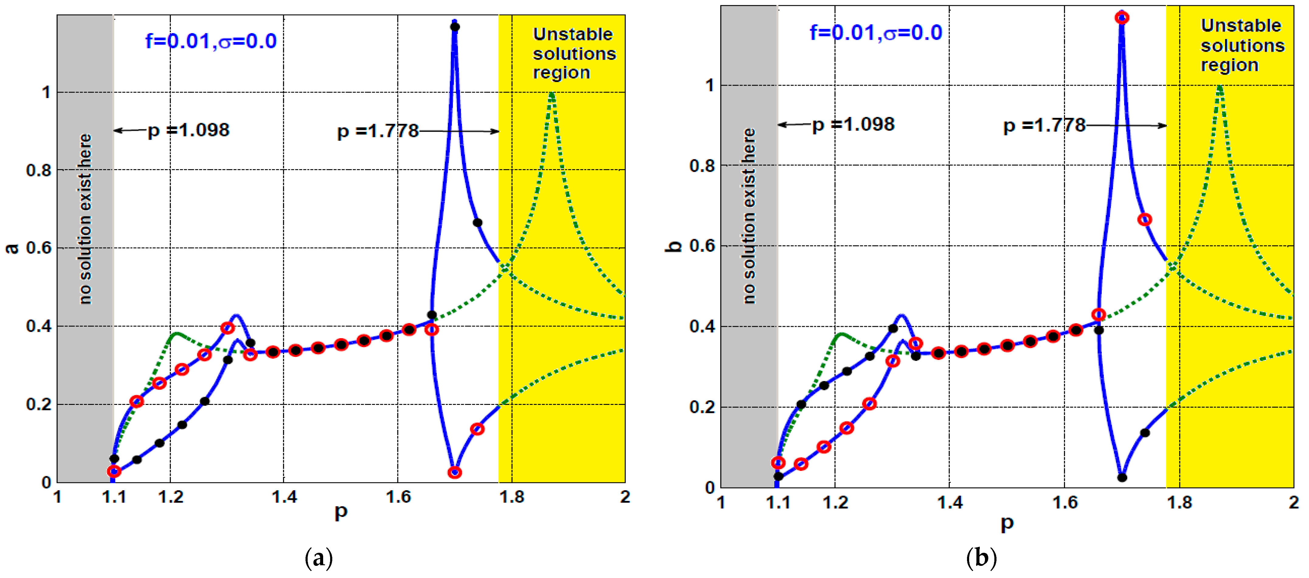
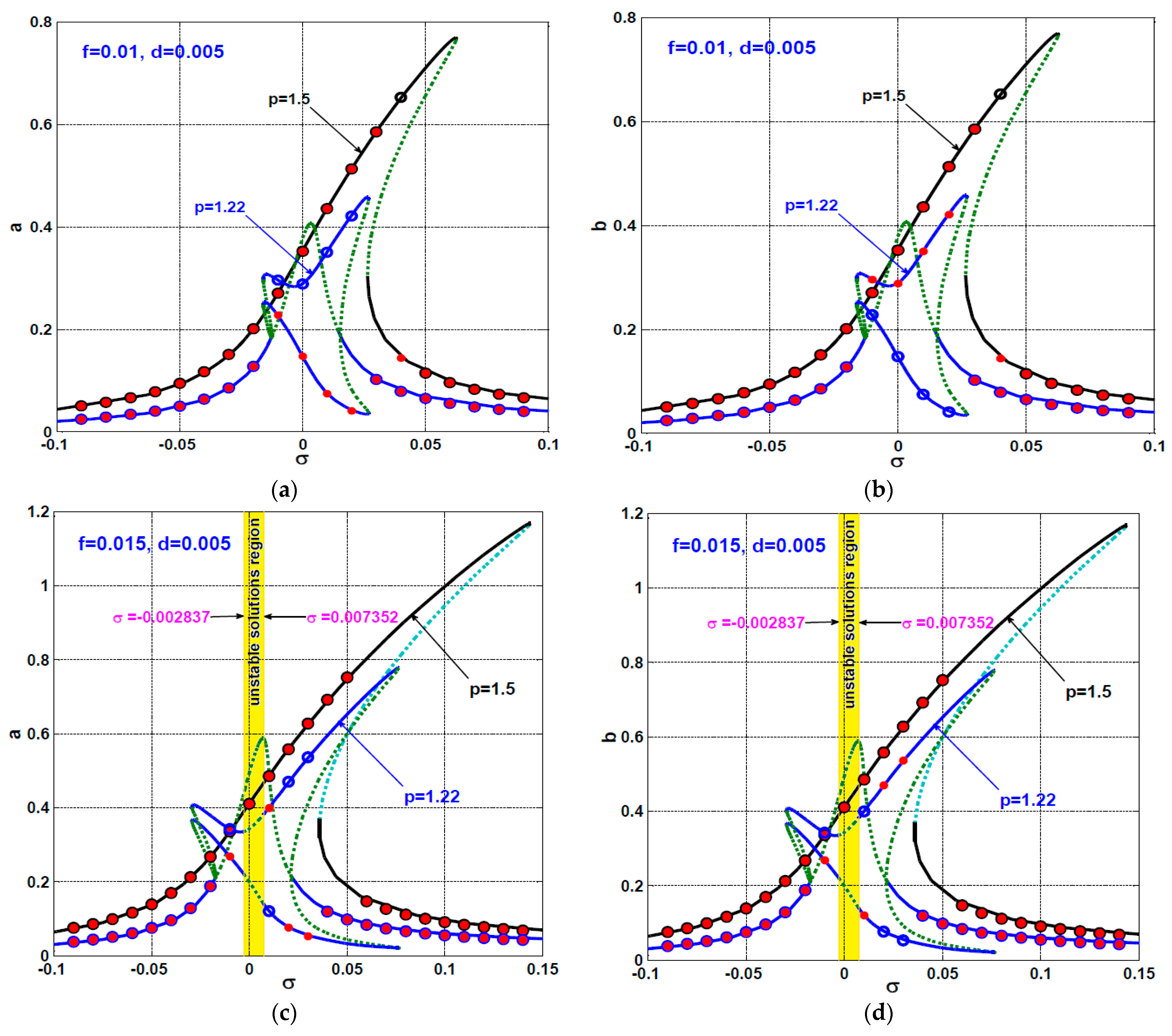
• The proportional gain has a great influence on the twelve-pole system’s dynamical behaviors, solution bifurcations, and stability conditions;
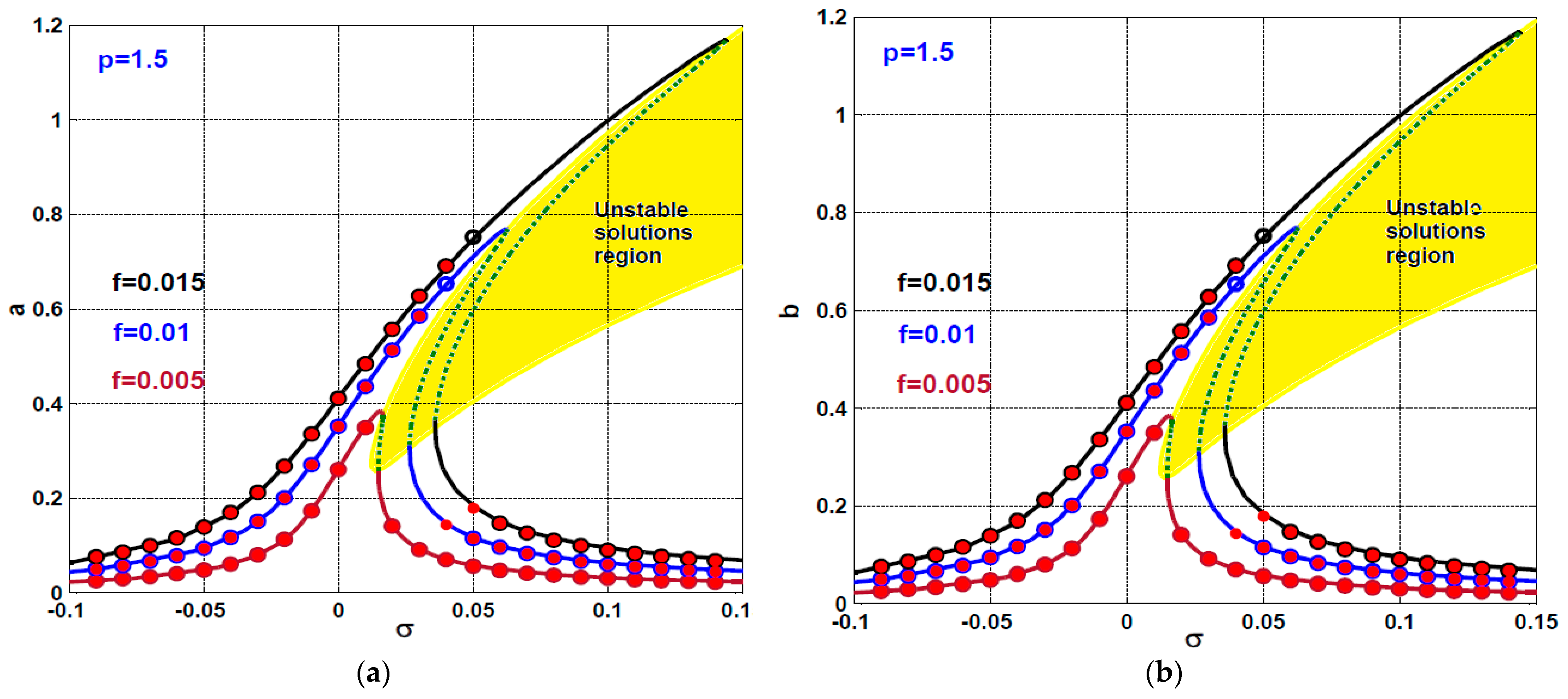
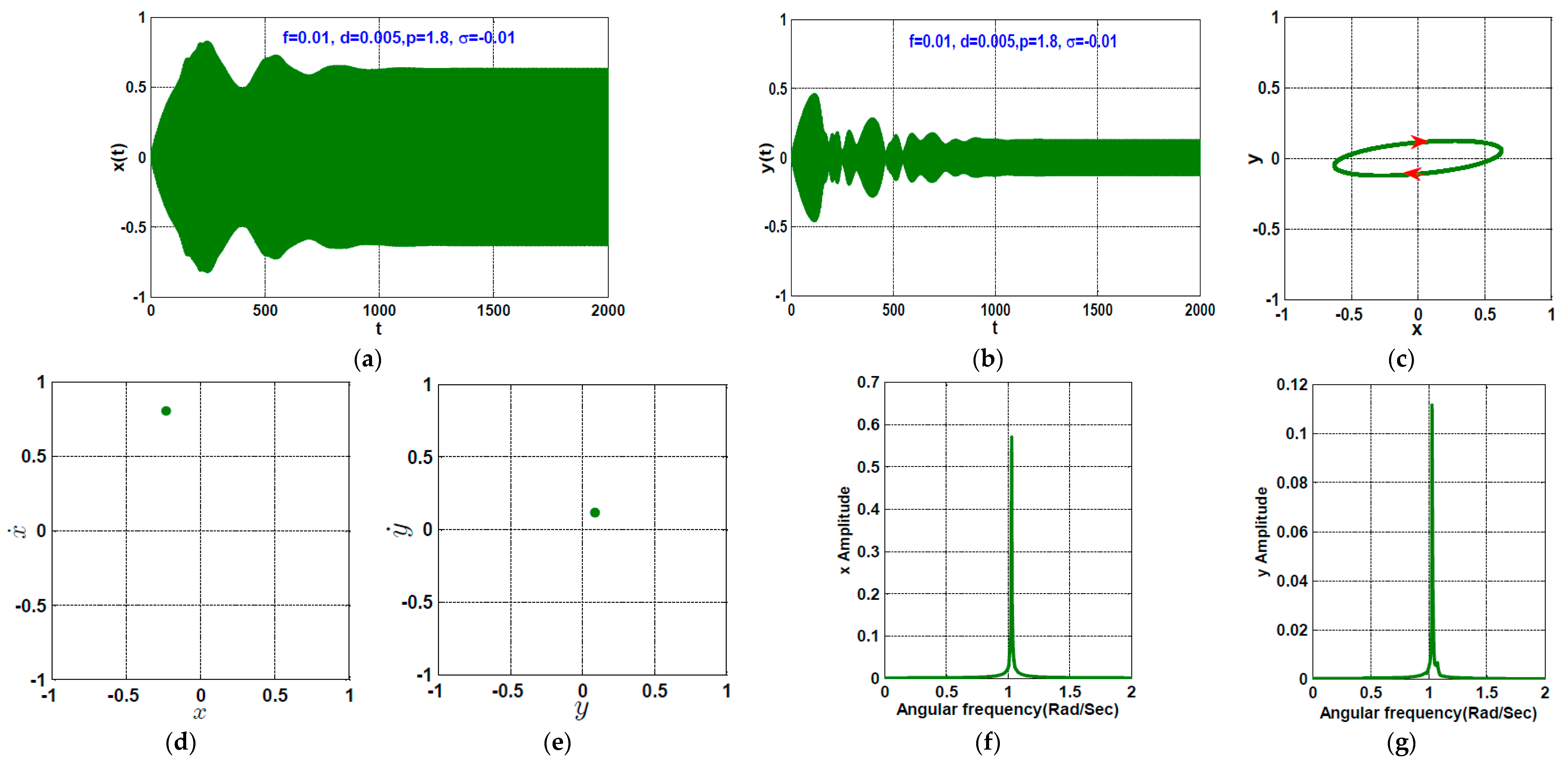
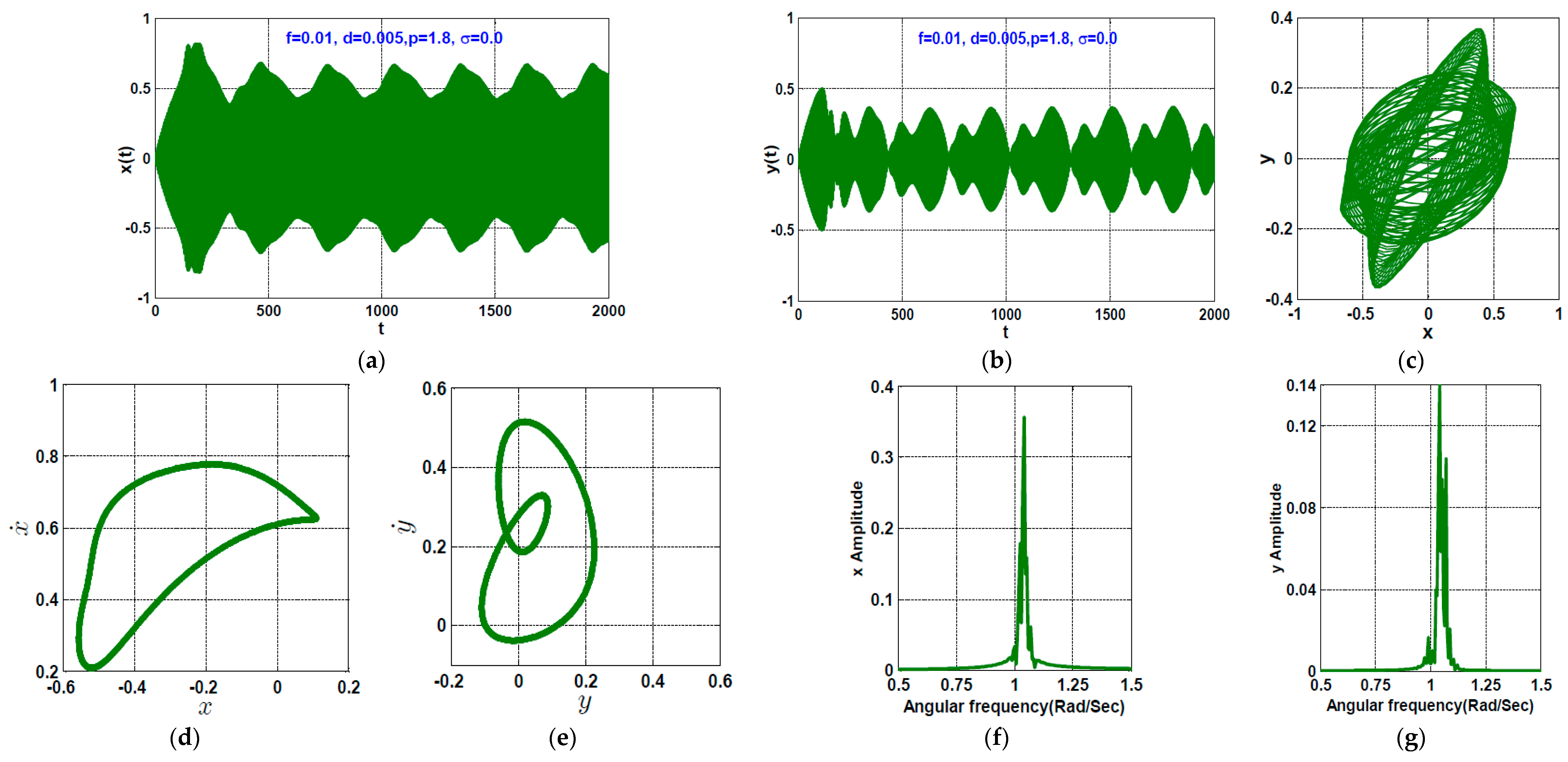
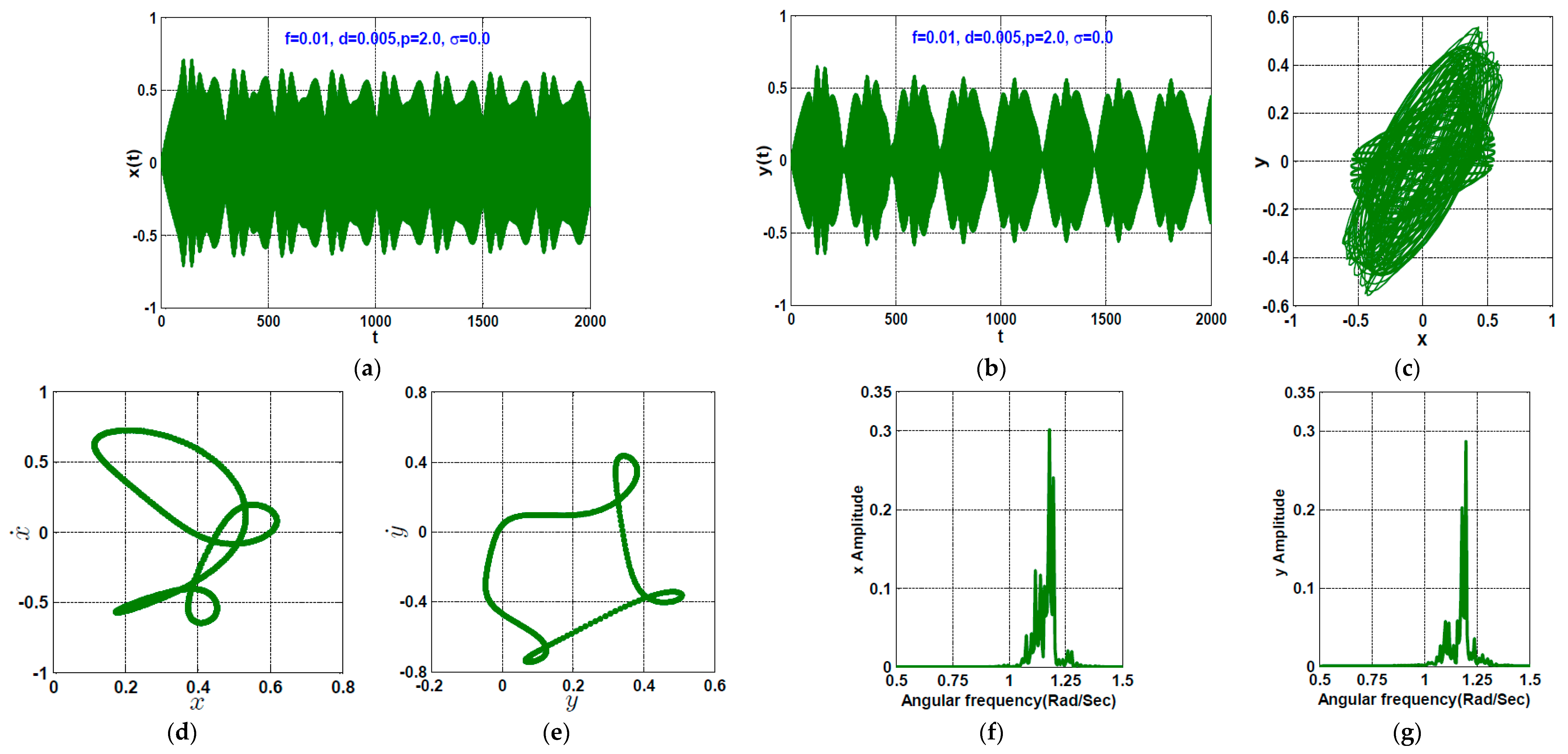
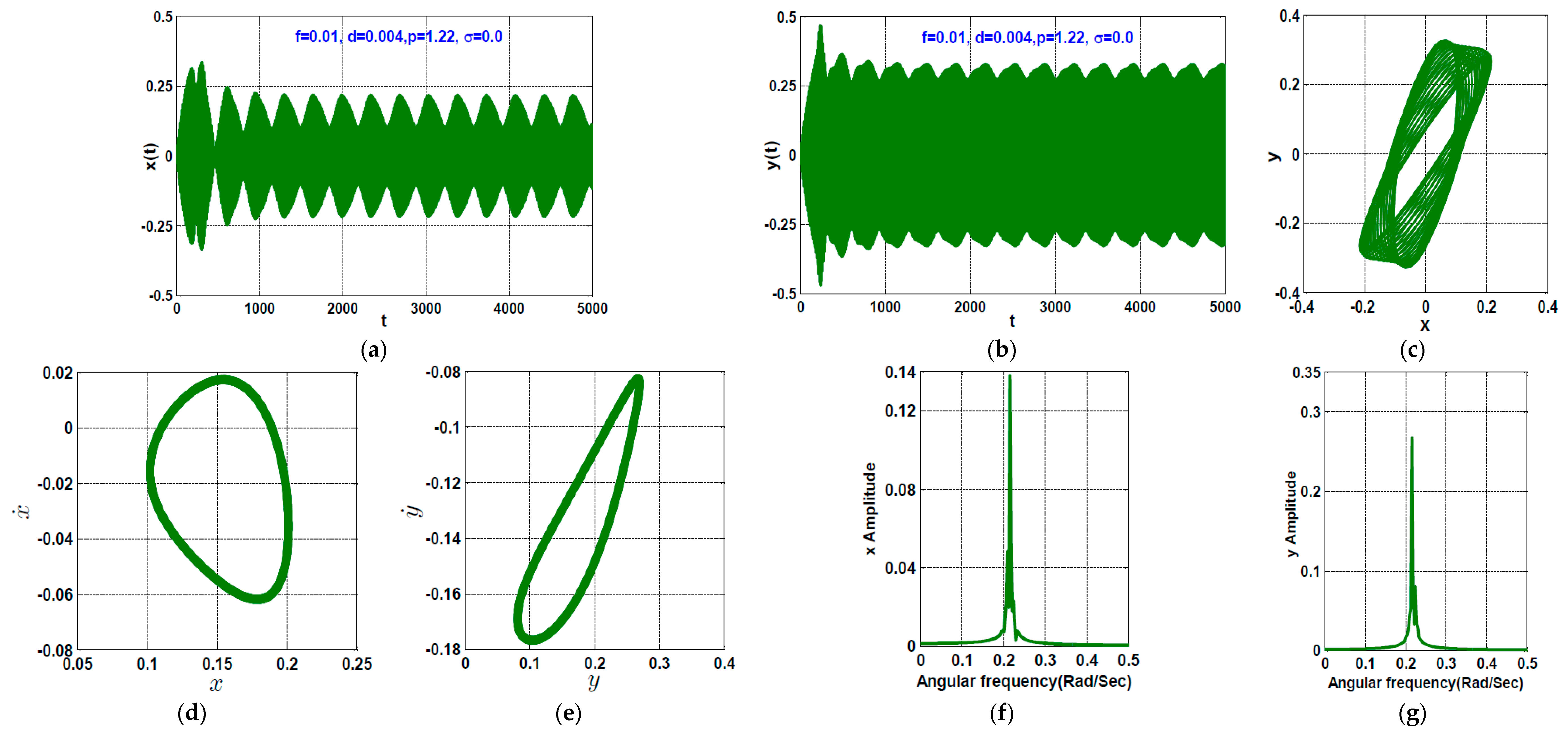
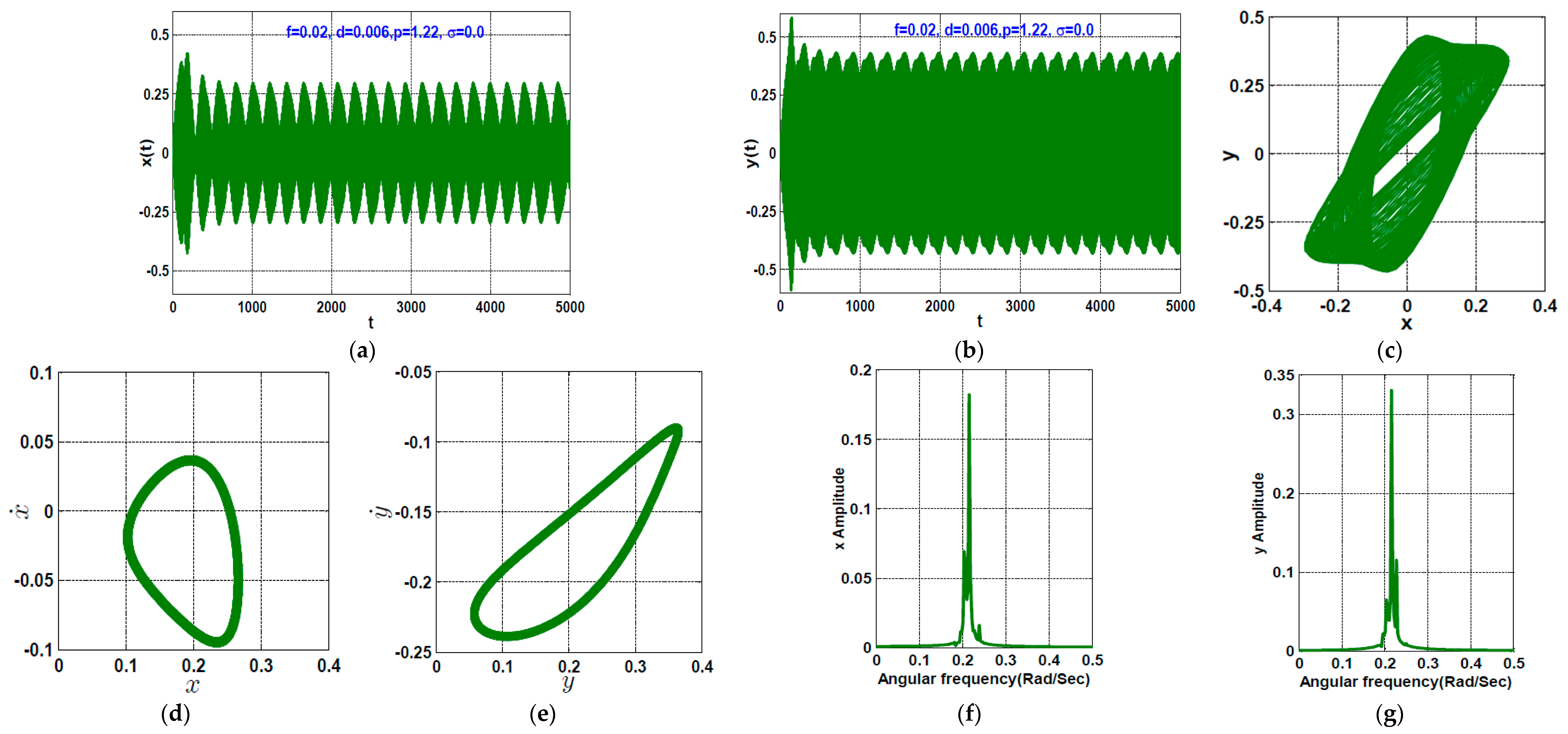
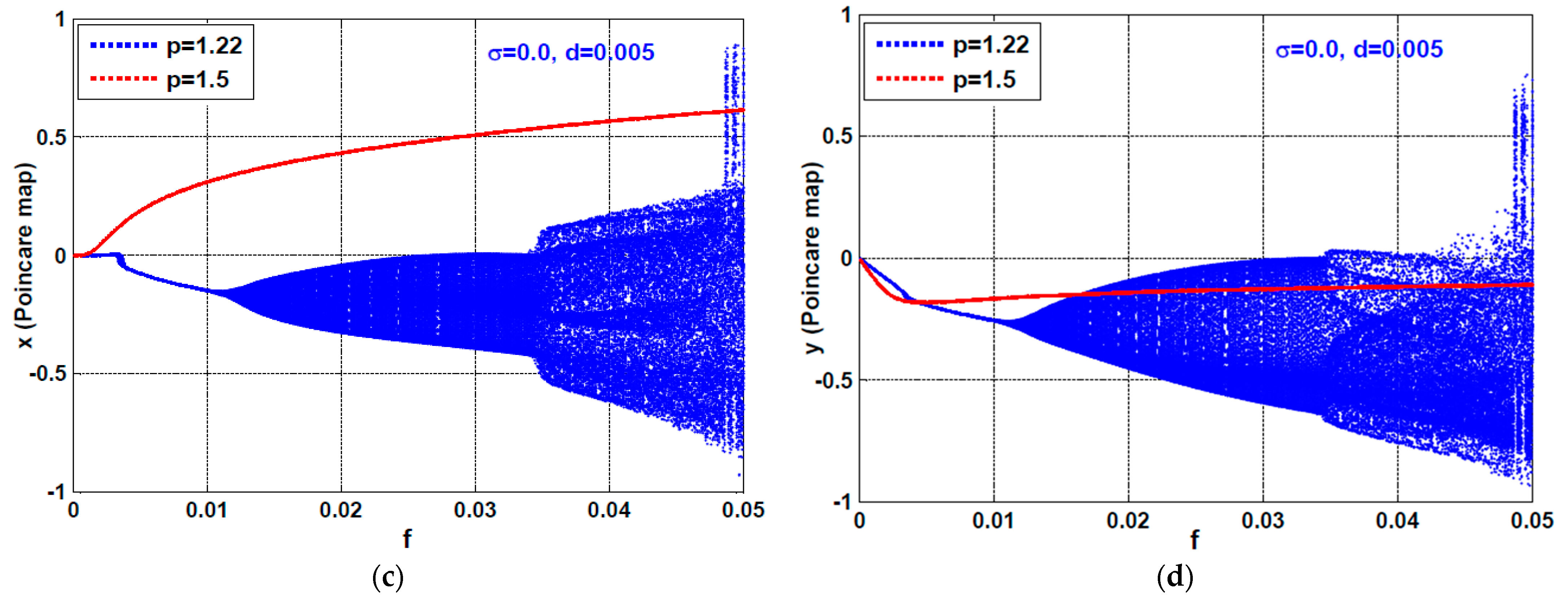
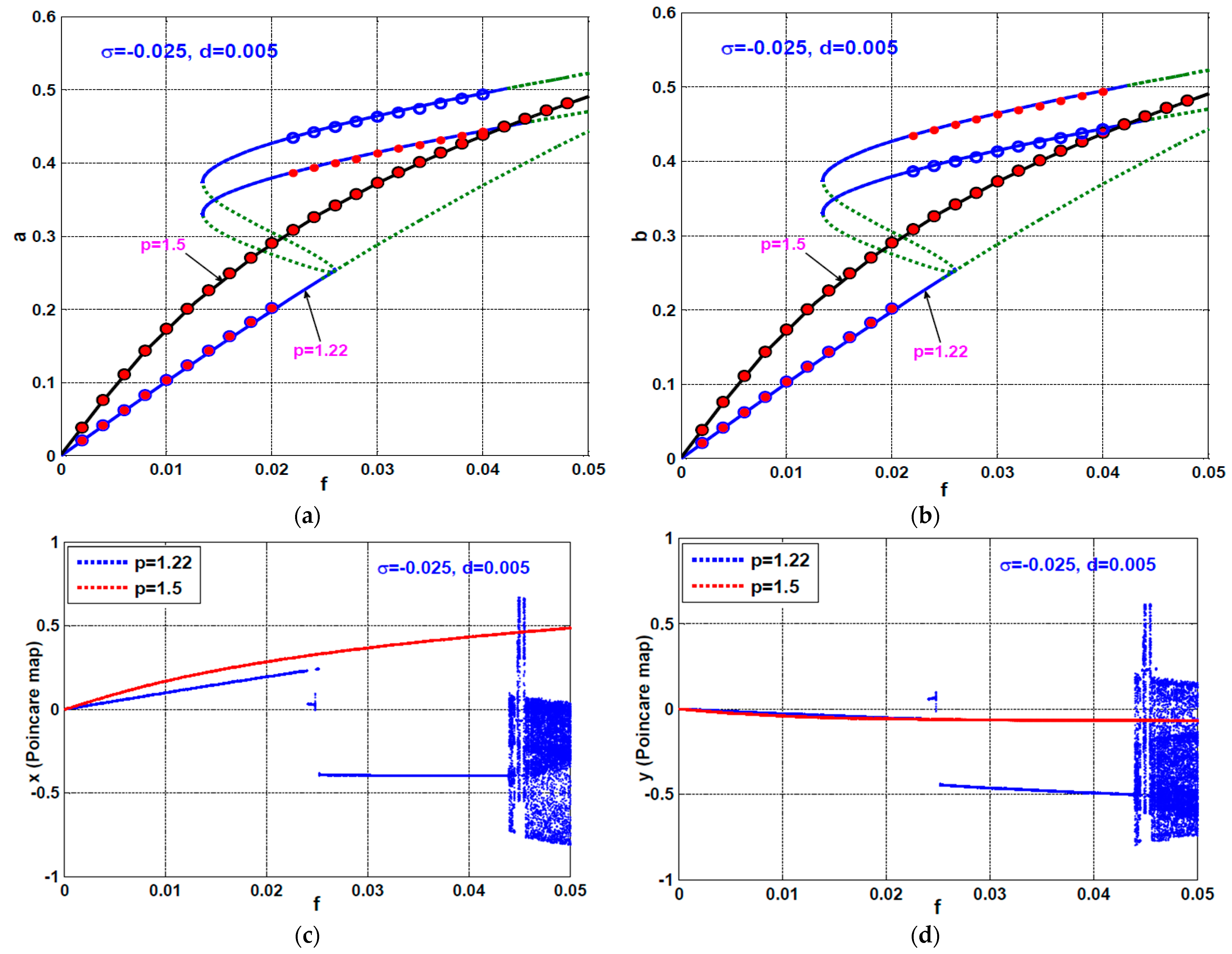
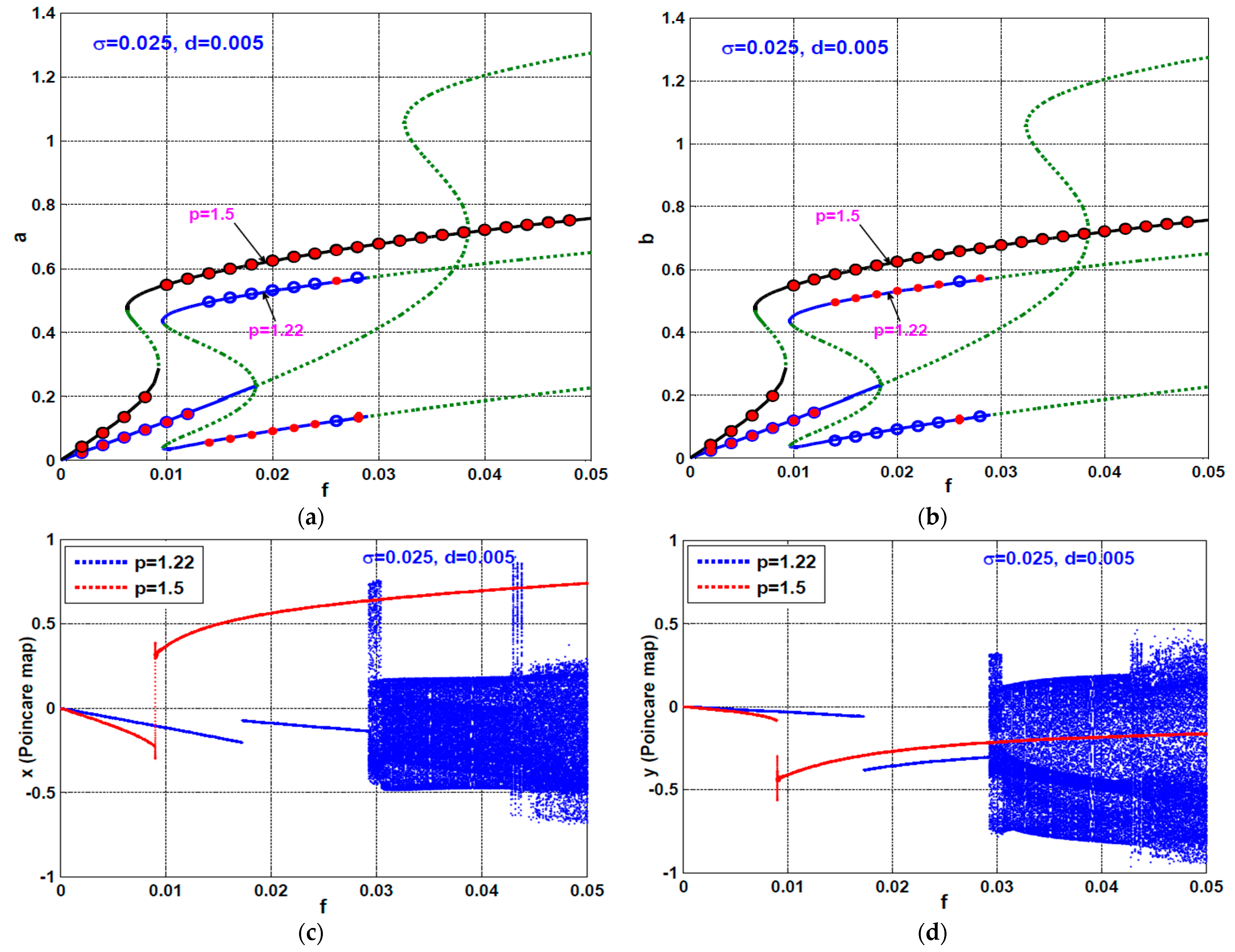
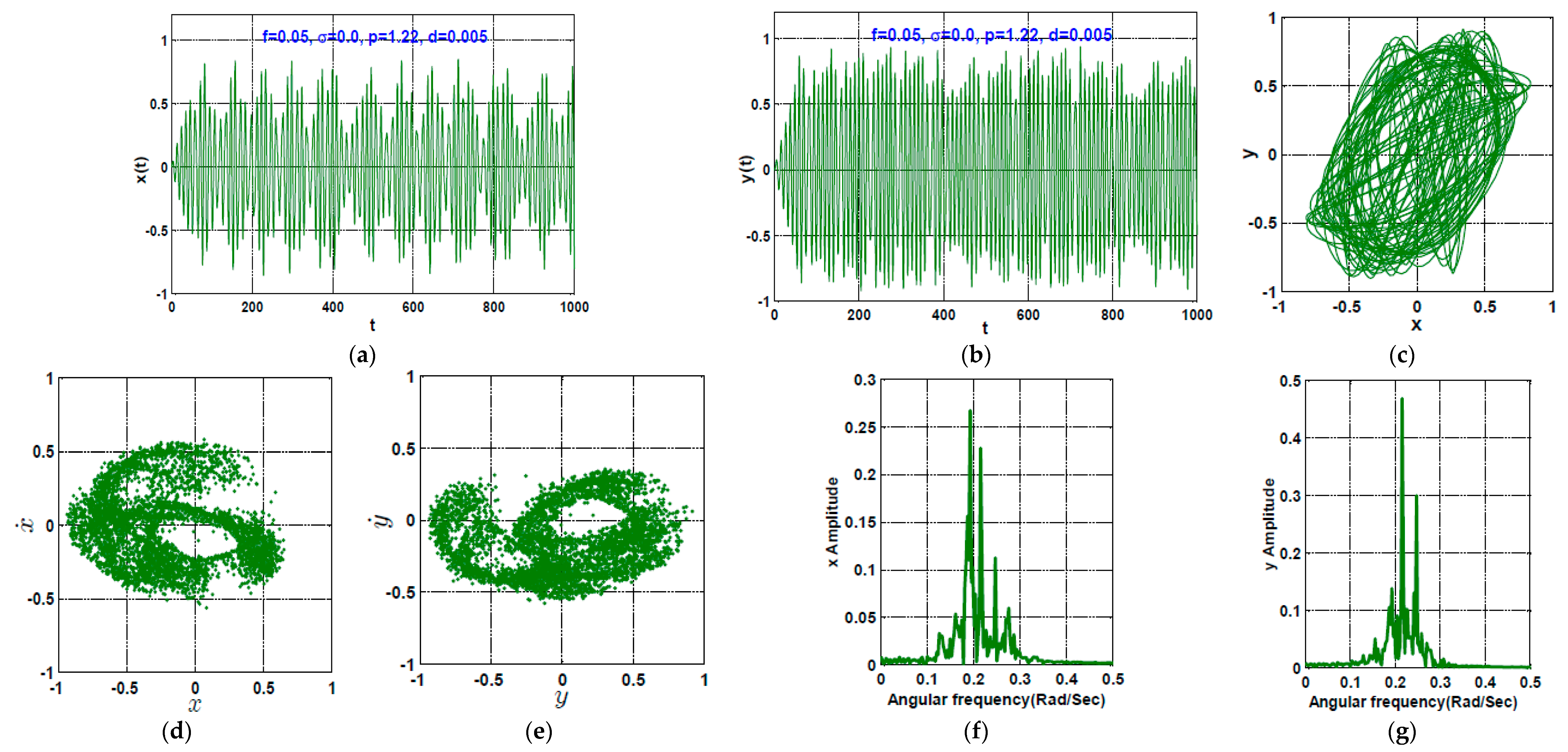
• At the small values of the proportional gain (i.e., $1.1<p<1.34$), the rotor system responds with a small oscillation amplitude with complex bifurcation behaviors at the small eccentricity magnitude $f$. However, the system may lose its stability to perform a quasiperiodic or chaotic oscillation when increasing the rotor eccentricity beyond a critical value;
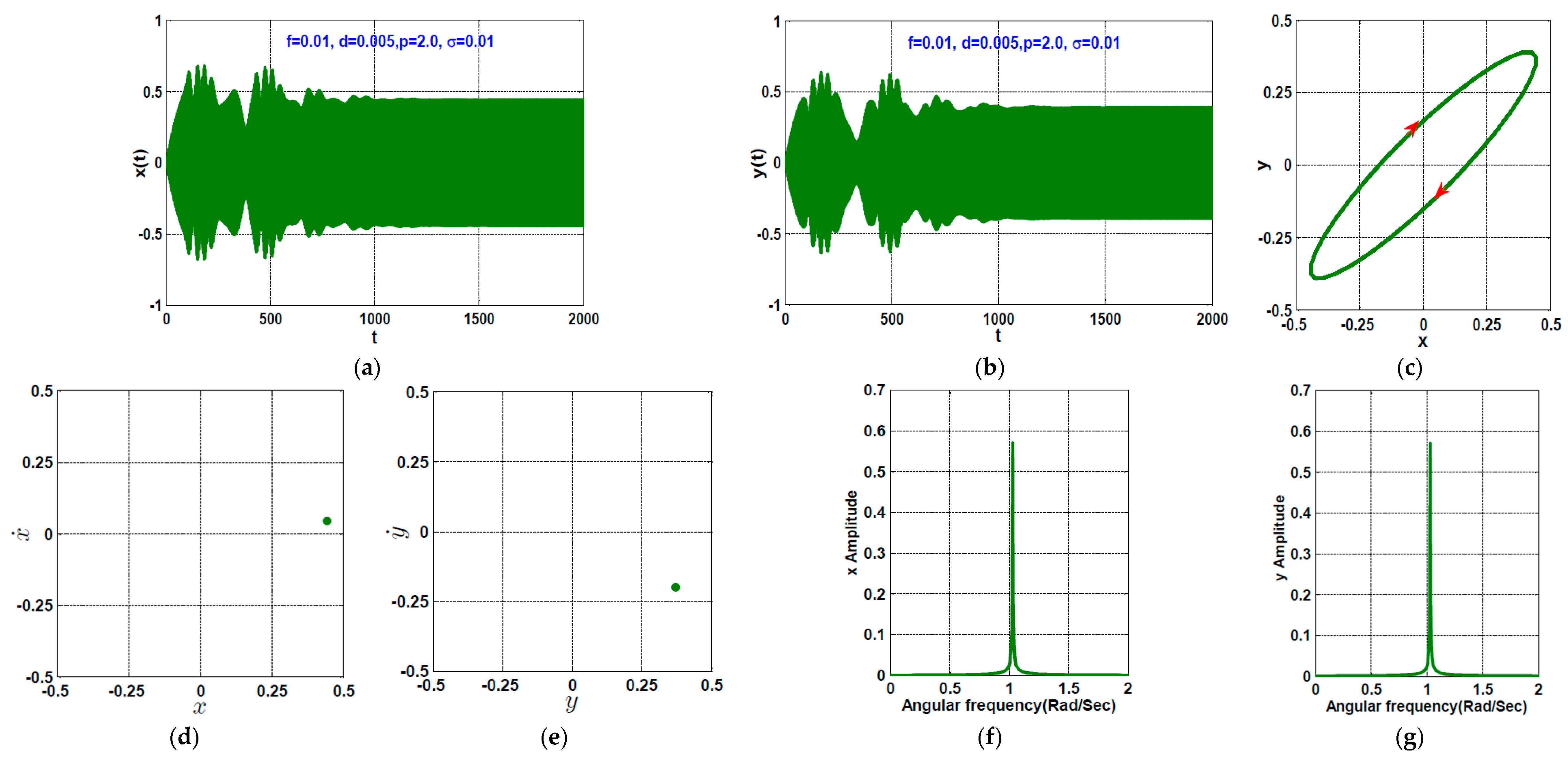
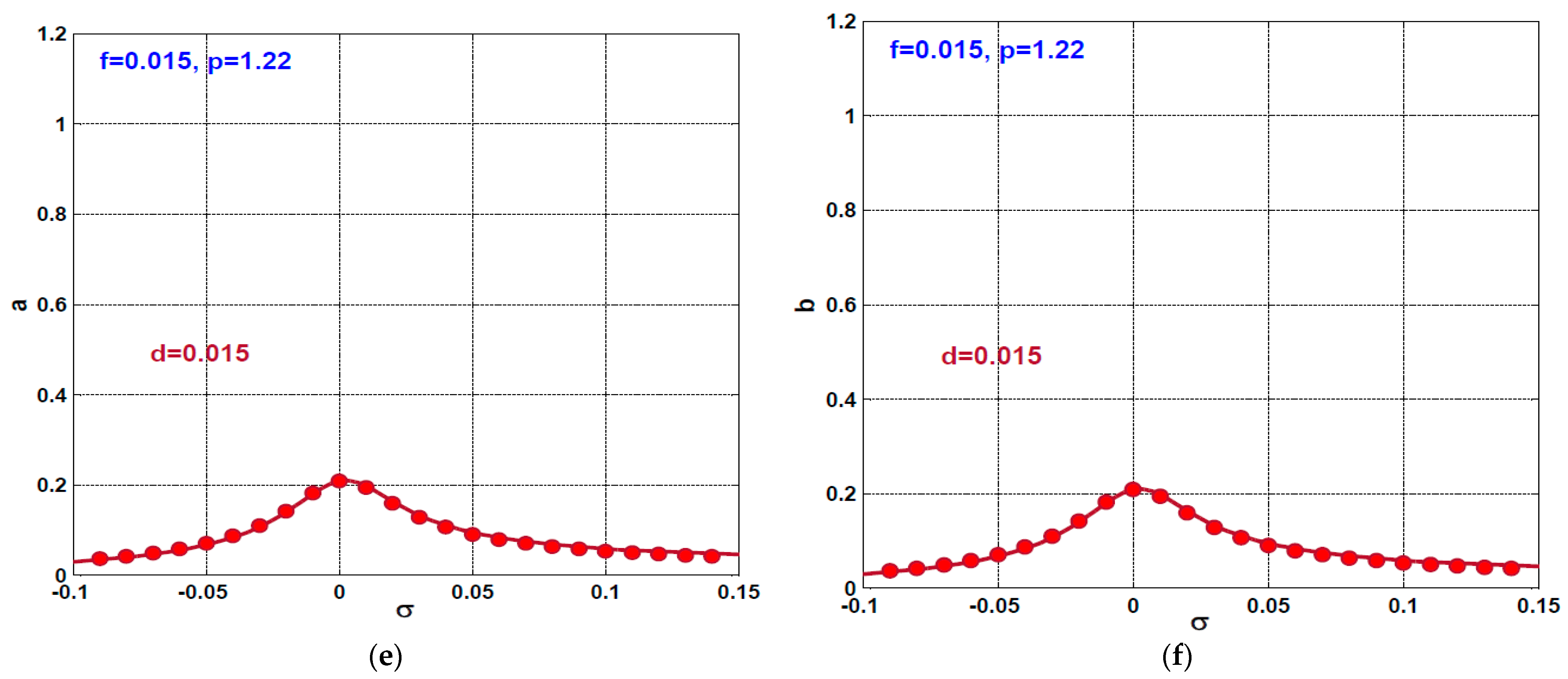
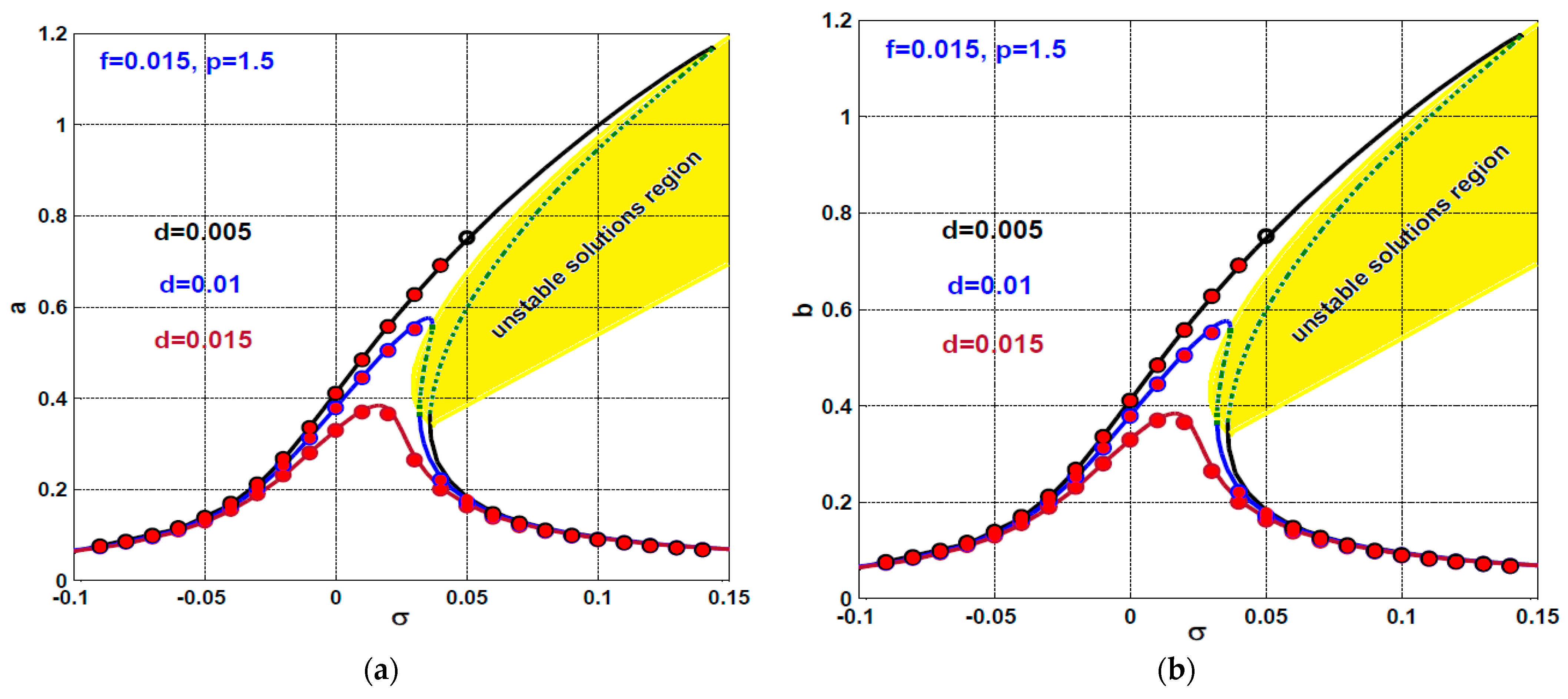
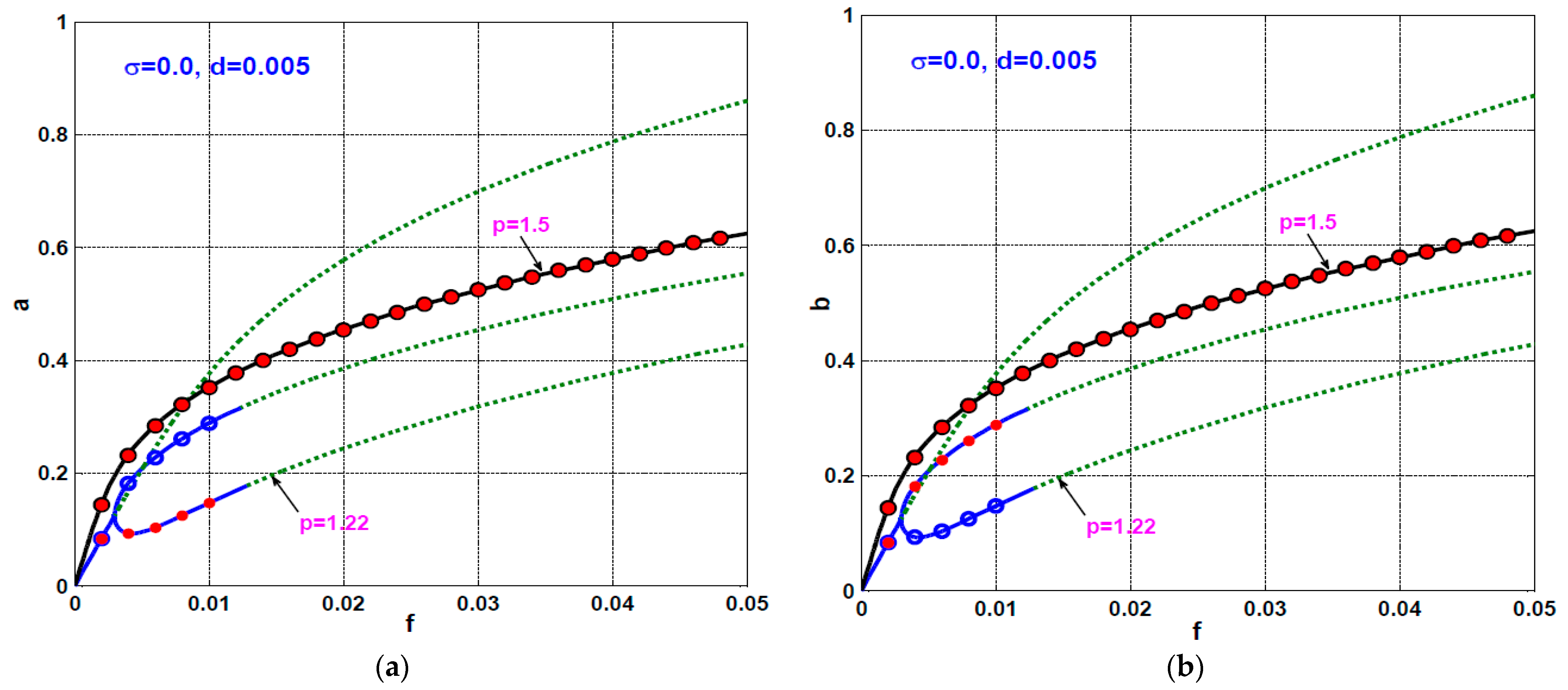
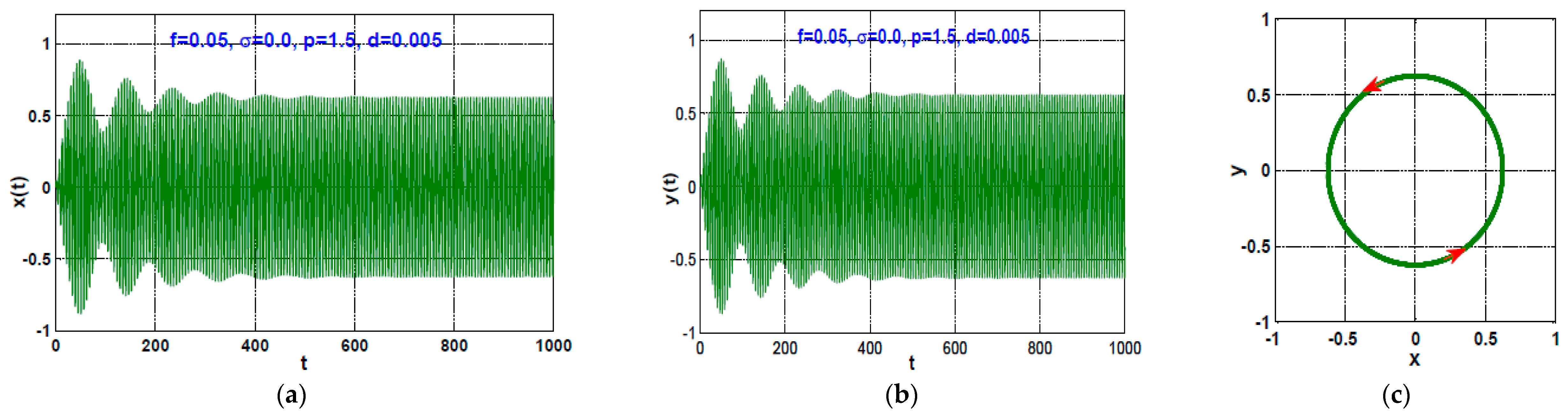
• At the large values of the proportional gain (i.e., when $1.34<p<1.65$), the twelve-pole rotor exhibits simple bifurcation behaviors and relatively large vibration amplitudes at the small disc eccentricities. In addition, the system responds periodically in the case of the strong values of the eccentricity $f$ without losing its stability;
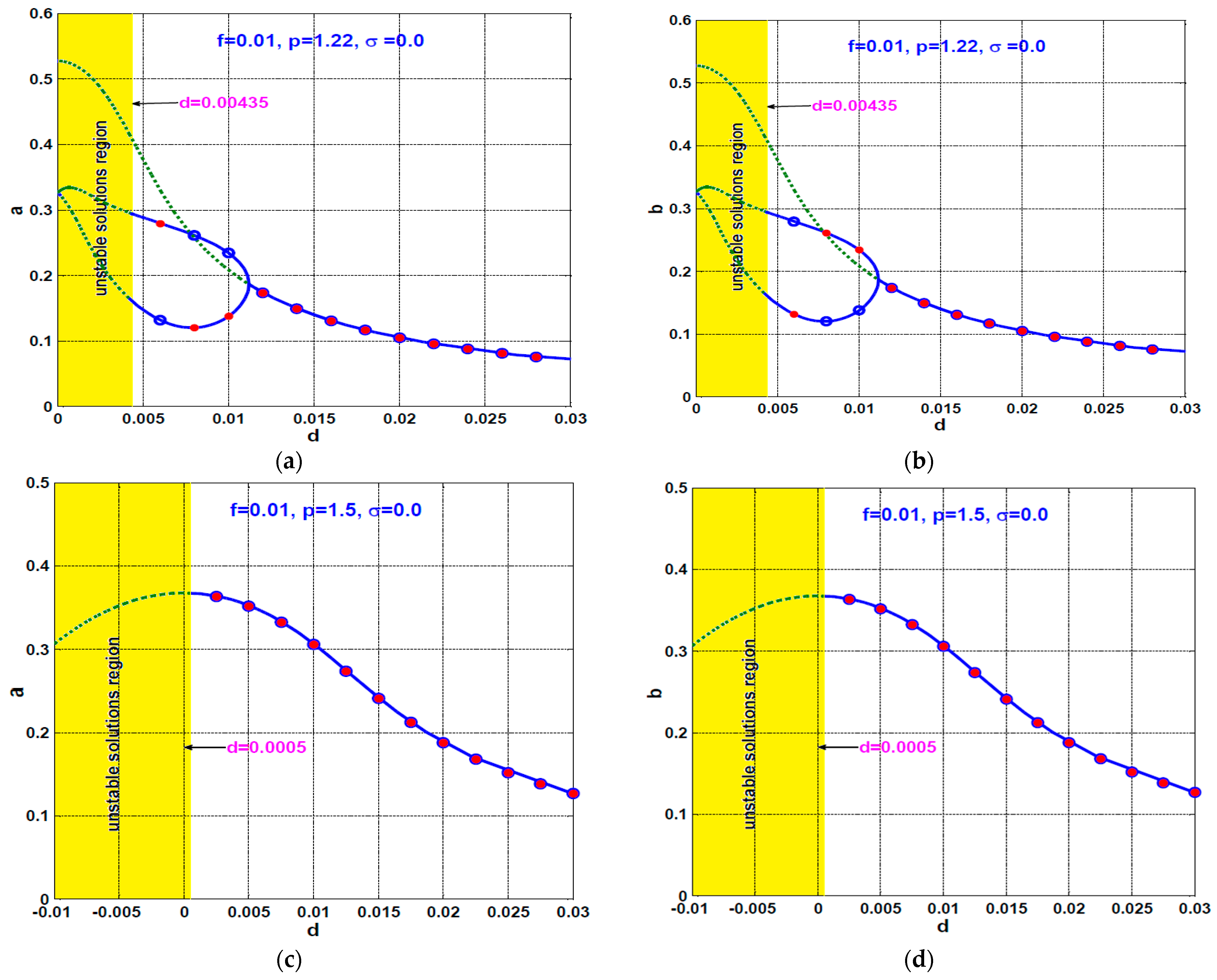
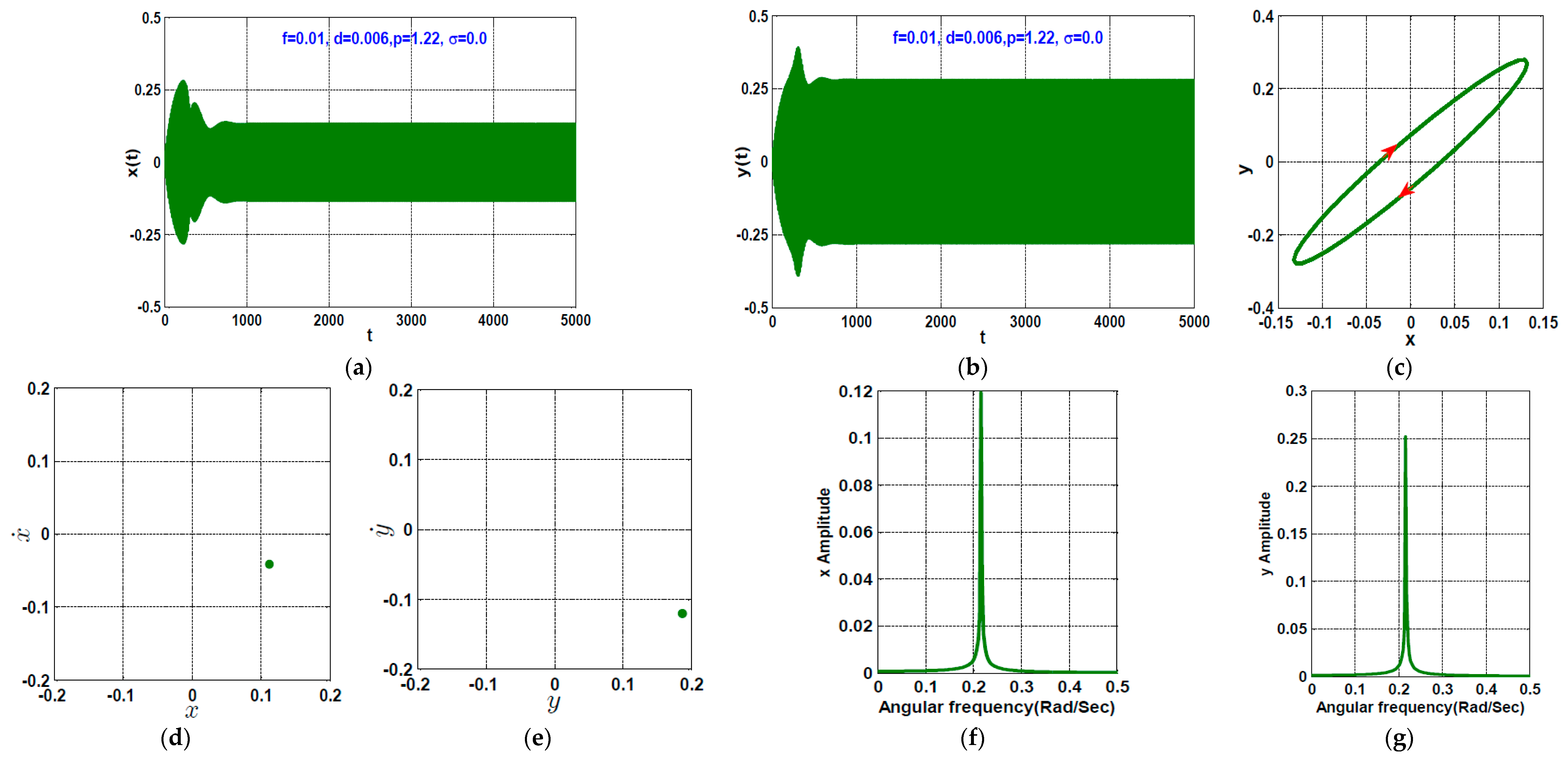
• Regardless of the proportional gain magnitude, the rotor system vibrations amplitudes are a monotonic decreasing function of the derivative gain, where increasing $d$ decreases the oscillation amplitudes and eliminate the motion bifurcations;
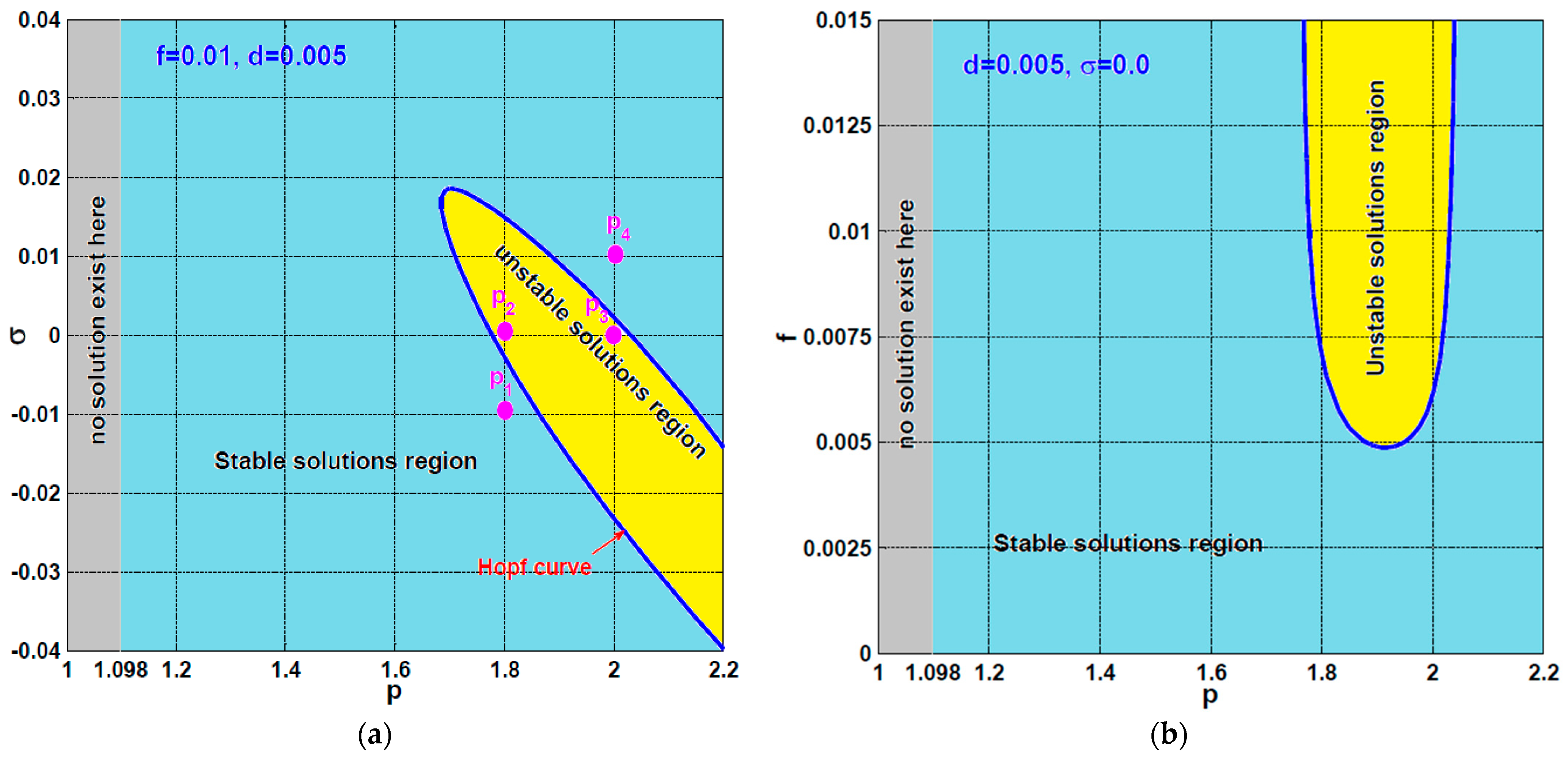
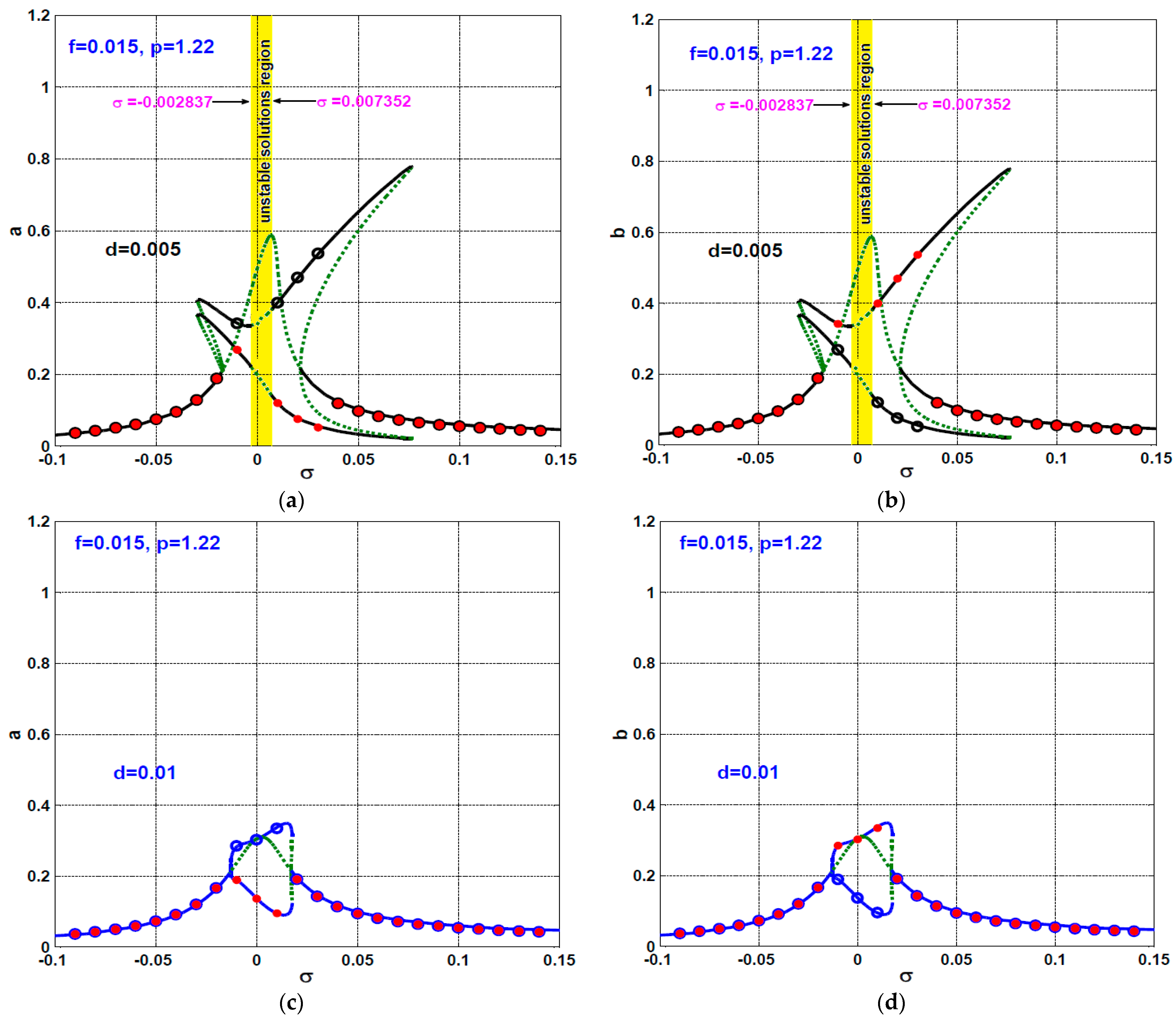
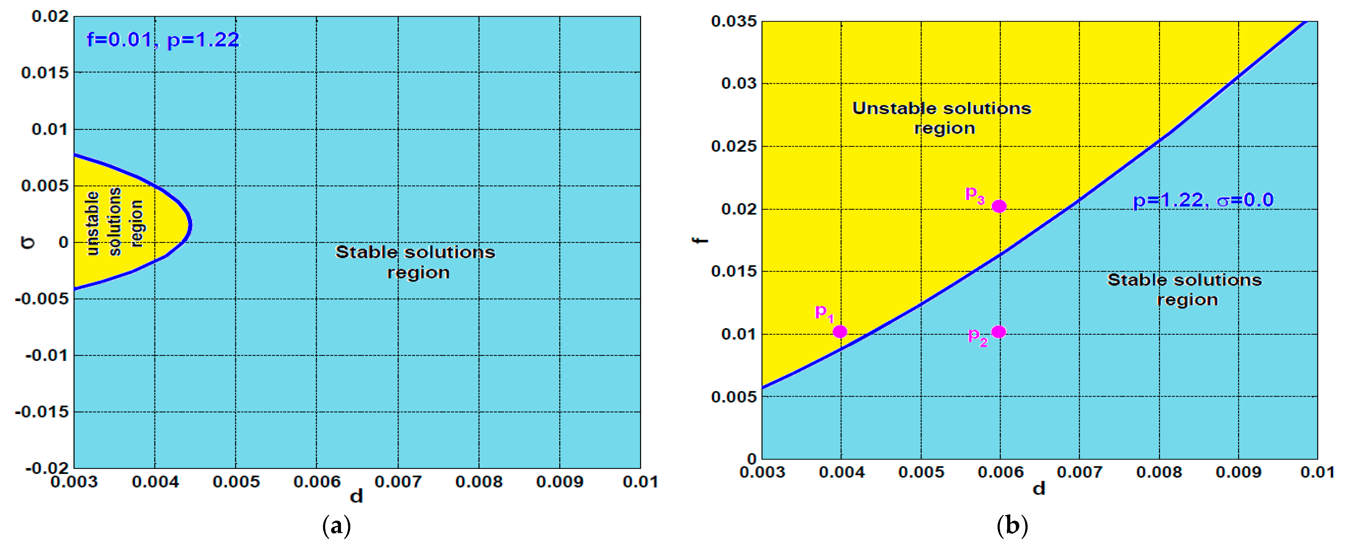
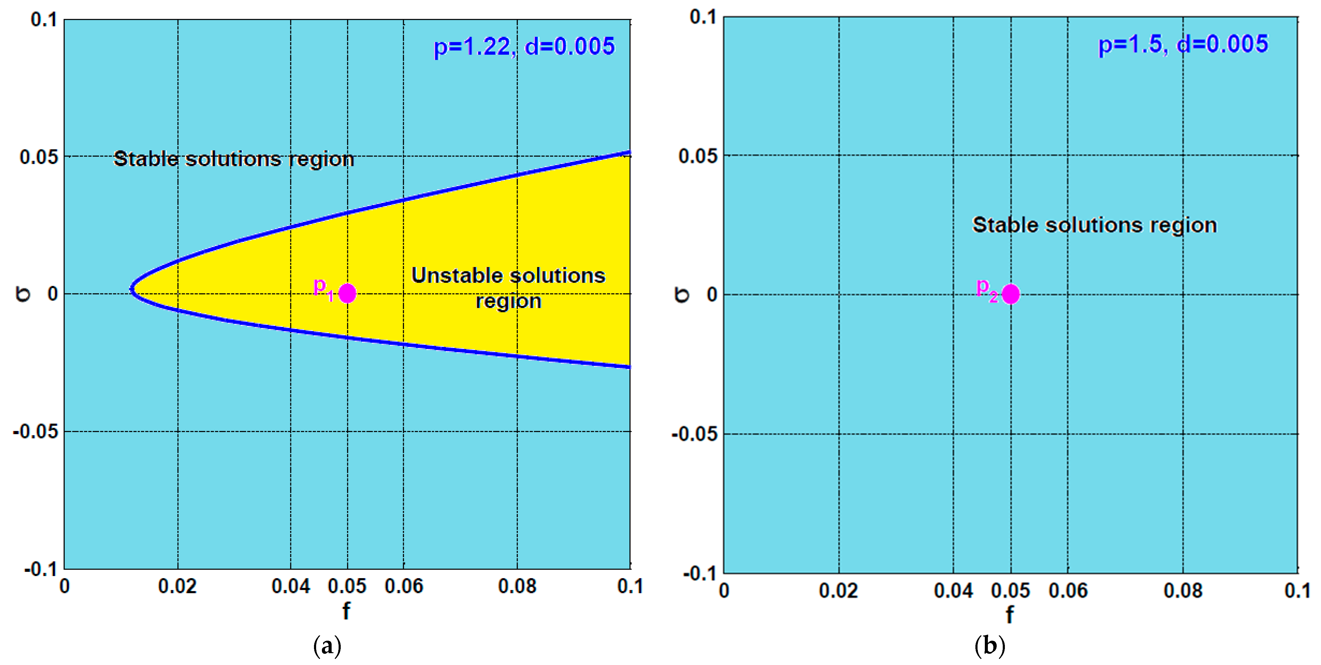
• The stability margin of the rotor eccentricity $f$ depends on the system angular speed $\Omega$ at the small values of the proportional gain (i.e., when $1.1<p<1.34$). However, the rotor system performs a stable periodic motion regardless of the eccentricity magnitude and rotor angular speed at the large values of the proportional gain (i.e., when $1.34<p<1.65$);
• The optimal design of the control variables ($p$ and $d$) is a compromising process that depends on the system parameters and the control objectives;
• It is recommended to investigate different advanced control methodologies for the twelve-pole system in future works.

References

1. Ji, J.C.; Yu, L.; Leung, A.Y.T. Bifurcation behavior of a rotor supported by active magnetic bearings. J. Sound Vib. 2000, 235, 133–151. [Google Scholar] [CrossRef]
2. Saeed, N.A.; Awwad, E.M.; El-Meligy, M.A.; Nasr, E.S.A. Radial Versus Cartesian Control Strategies to Stabilize the Nonlinear Whirling Motion of the Six-Pole Rotor-AMBs. IEEE Access 2020, 8, 138859–138883. [Google Scholar] [CrossRef]
3. Saeed, N.A.; Mahrous, E.; Awrejcewicz, J. Nonlinear dynamics of the six-pole rotor-AMBs under two different control configurations. Nonlinear Dyn. 2020, 101, 2299–2323. [Google Scholar] [CrossRef]
4. Ji, J.C.; Hansen, C.H. Non-linear oscillations of a rotor in active magnetic bearings. J. Sound Vib. 2001, 240, 599–612. [Google Scholar] [CrossRef]
5. Ji, J.C.; Leung, A.Y.T. Non-linear oscillations of a rotor-magnetic bearing system under superharmonic resonance conditions. Int. J. Nonlinear. Mech. 2003, 38, 829–835. [Google Scholar] [CrossRef]
6. Saeed, N.A.; Eissa, M.; El-Ganini, W.A. Nonlinear oscillations of rotor active magnetic bearings system. Nonlinear Dyn. 2013, 74, 1–20. [Google Scholar] [CrossRef]
7. Yang, X.D.; An, H.Z.; Qian, Y.J.; Zhang, W.; Yao, M.H. Elliptic Motions and Control of Rotors Suspending in Active Magnetic Bearings. J. Comput. Nonlinear Dyn. 2016, 11, 054503. [Google Scholar] [CrossRef]
8. Eissa, M.; Saeed, N.A.; El-Ganini, W.A. Saturation-based active controller for vibration suppression of a four-degree-of-freedom rotor-AMBs. Nonlinear Dyn. 2014, 76, 743–764. [Google Scholar] [CrossRef]
9. Saeed, N.A.; Kandil, A. Lateral vibration control and stabilization of the quasiperiodic oscillations for rotor-active magnetic bearings system. Nonlinear Dyn. 2019, 98, 1191–1218. [Google Scholar] [CrossRef]
10. Saeed, N.A.; Mahrous, E.; Abouel Nasr, E.; Awrejcewicz, J. Nonlinear dynamics and motion bifurcations of the rotor active magnetic bearings system with a new control scheme and rub-impact force. Symmetry 2021, 13, 1502. [Google Scholar] [CrossRef]
11. Zhang, W.; Zhan, X.P. Periodic and chaotic motions of a rotor-active magnetic bearing with quadratic and cubic terms and time-varying stiffness. Nonlinear Dyn. 2005, 41, 331–359. [Google Scholar] [CrossRef]
12. Zhang, W.; Yao, M.H.; Zhan, X.P. Multi-pulse chaotic motions of a rotor-active magnetic bearing system with time-varying stiffness. Chaos Solitons Fractals 2006, 27, 175–186. [Google Scholar] [CrossRef]
13. Zhang, W.; Zu, J.W.; Wang, F.X. Global bifurcations and chaos for a rotor-active magnetic bearing system with time-varying stiffness. Chaos Solitons Fractals 2008, 35, 586–608. [Google Scholar] [CrossRef]
14. Zhang, W.; Zu, J.W. Transient and steady nonlinear responses for a rotor-active magnetic bearings system with time-varying stiffness. Chaos Solitons Fractals 2008, 38, 1152–1167. [Google Scholar] [CrossRef]
15. Li, J.; Tian, Y.; Zhang, W.; Miao, S.F. Bifurcation of multiple limit cycles for a rotor-active magnetic bearings system with time-varying stiffness. Int. J. Bifurc. Chaos 2008, 18, 755–778. [Google Scholar] [CrossRef]
16. Li, J.; Tian, Y.; Zhang, W. Investigation of relation between singular points and number of limit cycles for a rotor–AMBs system. Chaos Solitons Fractals 2009, 39, 1627–1640. [Google Scholar] [CrossRef]
17. Saeed, N.A.; Kandil, A. Two different control strategies for 16-pole rotor active magnetic bearings system with constant stiffness coefficients. Appl. Math. Model. 2021, 92, 1–22. [Google Scholar] [CrossRef]
18. Kandil, A.; Sayed, M.; Saeed, N.A. On the nonlinear dynamics of constant stiffness coefficients 16-pole rotor active magnetic bearings system. Eur. J. Mech. A/Solids 2020, 84, 104051. [Google Scholar] [CrossRef]
19. Wu, R.; Zhang, W.; Yao, M.H. Nonlinear Vibration of a Rotor-Active Magnetic Bearing System with 16-Pole Legs. In Proceedings of the International Design Engineering Technical Conferences and Computers and Information in Engineering Conference, Cleveland, OH, USA, 6–9 August 2017. [Google Scholar] [CrossRef]
20. Wu, R.; Zhang, W.; Yao, M.H. Analysis of nonlinear dynamics of a rotor-active magnetic bearing system with 16-pole legs. In Proceedings of the International Design Engineering Technical Conferences and Computers and Information in Engineering Conference, Cleveland, OH, USA, 6–9 August 2017. [Google Scholar] [CrossRef]
21. Wu, R.Q.; Zhang, W.; Yao, M.H. Nonlinear dynamics near resonances of a rotor-active magnetic bearings system with 16-pole legs and time varying stiffness. Mech. Syst. Signal Process. 2018, 100, 113–134. [Google Scholar] [CrossRef]
22. Zhang, W.; Wu, R.Q.; Siriguleng, B. Nonlinear Vibrations of a Rotor-Active Magnetic Bearing System with 16-Pole Legs and Two Degrees of Freedom. Shock. Vib. 2020, 2020, 5282904. [Google Scholar] [CrossRef]
23. Ma, W.S.; Zhang, W.; Zhang, Y.F. Stability and multi-pulse jumping chaotic vibrations of a rotor-active magnetic bearing system with 16-pole legs under mechanical-electric-electromagnetic excitations. Eur. J. Mech. A/Solids 2021, 85, 104120. [Google Scholar] [CrossRef]
24. Ishida, Y.; Inoue, T. Vibration suppression of nonlinear rotor systems using a dynamic damper. J. Vib. Control 2007, 13, 1127–1143. [Google Scholar] [CrossRef]
25. Saeed, N.A.; Kamel, M. Active magnetic bearing-based tuned controller to suppress lateral vibrations of a nonlinear Jeffcott rotor system. Nonlinear Dyn. 2017, 90, 457–478. [Google Scholar] [CrossRef]
26. Saeed, N.A.; El-Ganaini, W.A. Time-delayed control to suppress the nonlinear vibrations of a horizontally suspended Jeffcott-rotor system. Appl. Math. Model. 2017, 44, 523–539. [Google Scholar] [CrossRef]
27. Saeed, N.A. On the steady-state forward and backward whirling motion of asymmetric nonlinear rotor system. Eur. J. Mech. A/Solids 2019, 80, 103878. [Google Scholar] [CrossRef]
28. Saeed, N.A. On vibration behavior and motion bifurcation of a nonlinear asymmetric rotating shaft. Arch. Appl. Mech. 2019, 89, 1899–1921. [Google Scholar] [CrossRef]
29. Saeed, N.A.; Awwad, E.M.; El-Meligy, M.A.; Nasr, E.S.A. Sensitivity analysis and vibration control of asymmetric nonlinear rotating shaft system utilizing 4-pole AMBs as an actuator. Eur. J. Mech. A/Solids 2021, 86, 104145. [Google Scholar] [CrossRef]
30. Saeed, N.A.; Awwad, E.M.; El-Meligy, M.A.; Nasr, E.S.A. Analysis of the rub-impact forces between a controlled nonlinear rotating shaft system and the electromagnet pole legs. Appl. Math. Model. 2021, 93, 792–810. [Google Scholar] [CrossRef]
31. Saeed, N.A.; El-Bendary, S.I.; Sayed, M.; Mohamed, M.S.; Elagan, S.K. On the oscillatory behaviours and rub-impact forces of a horizontally supported asymmetric rotor system under position-velocity feedback controller. Lat. Am. J. Solids Struct. 2021, 18, e349. [Google Scholar] [CrossRef]
32. Saeed, N.A.; Awwad, E.M.; Maarouf, A.; Farh, H.M.H.; Alturki, F.A.; Awrejcewicz, J. Rub-impact force induces periodic, quasiperiodic, and chaotic motions of a controlled asymmetric rotor system. Shock. Vib. 2021, 2021, 1800022. [Google Scholar] [CrossRef]
33. Srinivas, R.S.; Tiwari, R.; Kannababu, C. Application of active magnetic bearings in flexible rotordynamic systems—A state-of-the-art review. Mech. Syst. Signal Process. 2018, 106, 537–572. [Google Scholar] [CrossRef]
34. Chittlangia, V.; Lijesh, K.P.; Akash, K.; Hirani, H. Optimum design of an active magnetic bearing considering the geometric programming. Technol. Lett. 2014, 1, 23–30. [Google Scholar]
35. Kumar, G.; Choudhury, M.D.; Natesan, S.; Kalita, K. Design and analysis of a radial active magnetic bearing for vibration control. Procedia Eng. 2016, 144, 810–816. [Google Scholar] [CrossRef] [Green Version]
36. Zhang, W.; Zhu, H. Radial magnetic bearings: An overview. Results Phys. 2017, 7, 3756–3766. [Google Scholar] [CrossRef]
37. Zhong, Z.; Duan, Y.; Cai, Z.; Qi, Y. Design and cosimulation of twelve-pole heteropolar radial hybrid magnetic bearing. Math. Probl. Eng. 2021, 2021, 8826780. [Google Scholar] [CrossRef]
38. Ishida, Y.; Yamamoto, T. Linear and Nonlinear Rotordynamics: A Modern Treatment with Applications, 2nd ed.; Wiley-VCH Verlag GmbH & Co. KGaA: New York, NY, USA, 2012. [Google Scholar] [CrossRef]
39. Schweitzer, G.; Maslen, E.H. Magnetic Bearings: Theory, Design, and Application to Rotating Machinery; Springer: Berlin/Heidelberg, Germany, 2009. [Google Scholar] [CrossRef]
40. Nayfeh, A.H.; Mook, D.T. Nonlinear Oscillations; Wiley: New York, NY, USA, 1995. [Google Scholar] [CrossRef]
Figure 1. Closed-loop control system of active magnetic bearings system.
Applsci 11 10839 g001
Figure 2. Twelve-pole rotor system: (a) three-dimensional 12-pole system, and (b) the 12-pole system schematic diagram.
Applsci 11 10839 g002
Figure 3. Oscillation amplitudes of the twelve-pole system versus σ at p = 1.22 : (a,b) f = 0.005 , (c,d) f = 0.01 , and (e,f) f = 0.015 .
Applsci 11 10839 g003
Figure 4. Oscillation amplitudes of the twelve-pole system versus σ at f = 0.01 : (a,b) p = 1.4 , and (c,d) p = 1.5 .
Applsci 11 10839 g004
Figure 5. Oscillation amplitudes of the twelve-pole system versus σ at p = 1.5 when f = 0.005 ,   0.01 and 0.015 : (a) oscillation amplitude in X -direction, (b) oscillation amplitude in Y -direction.
Applsci 11 10839 g005
Figure 6. Oscillation amplitudes of the twelve-pole system versus p at σ = 0.0 ,   d = 0.005 , and f = 0.01 : (a) oscillation in X -direction, (b) oscillation in Y -direction.
Applsci 11 10839 g006
Figure 7. Stability chart of the twelve-pole system: (a) p σ plane when d = 0.005 and f = 0.01 , (b) p f plane when d = 0.005 and σ = 0 . .
Applsci 11 10839 g007
Figure 8. Numerical simulation for the twelve-pole system according to the marked point p 1 in Figure 6a (i.e., when p = 1.8 , σ = 0.01 ): (a,b) temporal oscillations, (c) orbital motion, (d,e) Poincaré return map, and (f,g) frequency spectrum.
Applsci 11 10839 g008
Figure 9. Numerical simulation for the twelve-pole system according to the marked point p 2 in Figure 6a (i.e., when p = 1.8 , σ = 0.0 ): (a,b) temporal oscillations, (c) orbital motion, (d,e) Poincaré return map, and (f,g) frequency spectrum.
Applsci 11 10839 g009
Figure 10. Numerical simulation for the twelve-pole system according to the marked point p 3 in Figure 6a (i.e., when p = 2.0 , σ = 0.0 ): (a,b) temporal oscillations, (c) orbital motion, (d,e) Poincaré return map, and (f,g) frequency spectrum.
Applsci 11 10839 g010
Figure 11. Numerical simulation for the twelve-pole system according to the marked point p 4 in Figure 6a (i.e., when p = 2.0 , σ = 0.01 ): (a,b) temporal oscillation, (c) orbital motion, (d,e) Poincaré return map, and (f,g) frequency spectrum.
Applsci 11 10839 g011
Figure 12. Oscillation amplitudes of the twelve-pole system versus σ at f = 0.015 and p = 1.22 : (a,b) d = 0.005 , (c,d) d = 0.01 , and (e,f) d = 0.015 .
Applsci 11 10839 g012aApplsci 11 10839 g012b
Figure 13. Oscillation amplitudes of the twelve-pole system versus σ at p = 1.5 ,   f = 0.015 when d = 0.005 ,   0.01 and 0.015 : (a) oscillation in X -direction, (b) oscillation in Y -direction.
Applsci 11 10839 g013
Figure 14. Oscillation amplitudes of the twelve-pole system versus d when σ = 0.0   and f = 0.01 : (a,b) p = 1.22 , and (c,d) p = 1.5 .
Applsci 11 10839 g014
Figure 15. Stability chart of the twelve-pole system: (a) d σ plane when f = 0.01 and p = 1.22 , and (b) d f plane when p = 1.22 and σ = 0 .
Applsci 11 10839 g015
Figure 16. Numerical simulation for the twelve-pole system according to the marked point p 1 in Figure 14b (i.e., when d = 0.004 , f = 0.01 ): (a,b) temporal oscillation, (c) orbital motion, (d,e) Poincaré return map, and (f,g) frequency spectrum.
Applsci 11 10839 g016
Figure 17. Numerical simulation for the twelve-pole system according to the marked point p 2 in Figure 14b (i.e., when d = 0.006 , f = 0.01 ): (a,b) temporal oscillation, (c) orbital motion, (d,e) Poincaré return map, and (f,g) frequency spectrum.
Applsci 11 10839 g017
Figure 18. Numerical simulation for the twelve-pole system according to the marked point p 3 in Figure 14b (i.e., when d = 0.006 , f = 0.02 ): (a,b) temporal oscillation, (c) orbital motion, (d,e) Poincaré return map, and (f,g) frequency spectrum.
Applsci 11 10839 g018
Figure 19. (a,b) Oscillation amplitudes of the twelve-pole system versus f , and (c,d) the corresponding bifurcation diagrams at σ = 0.0 ,   d = 0.005 when p = 1.22 and 1.5 .
Applsci 11 10839 g019aApplsci 11 10839 g019b
Figure 20. (a,b) Oscillation amplitudes of the twelve-pole system versus f , and (c,d) the corresponding bifurcation diagrams at σ = 0.025 ,   d = 0.005 when p = 1.22 and 1.5 .
Applsci 11 10839 g020
Figure 21. (a,b) Oscillation amplitudes of the twelve-pole system versus f , and (c,d) the corresponding bifurcation diagrams at σ = 0.025 ,   d = 0.005 when p = 1.22 and 1.5 .
Applsci 11 10839 g021
Figure 22. Stability chart of the twelve-pole system: (a) f σ plane when p = 1.22 and d = 0.005 , and (b) f σ plane when p = 1.5 and d = 0.005 .
Applsci 11 10839 g022
Figure 23. Numerical simulation for the twelve-pole system according to the marked point p 1 in Figure 21a (i.e., when f = 0.05 , σ = 0.0 , p = 1.22 ): (a,b) temporal oscillation, (c) orbital motion, (d,e) Poincaré return map, and (f,g) frequency spectrum.
Applsci 11 10839 g023
Figure 24. Numerical simulation for the twelve-pole system according to the marked point p 2 in Figure 21b (i.e., when f = 0.05 , σ = 0.0 ,   p = 1.5 ): (a,b) temporal oscillation, and (c) orbital motion.
Applsci 11 10839 g024
Figure 25. Oscillation amplitudes of the twelve-pole system versus σ at d = 0.005 , when p = 1.22   and 1.5 : (a,b) f = 0.01 , and (c,d) f = 0.015 .
Applsci 11 10839 g025
Publisher’s Note: MDPI stays neutral with regard to jurisdictional claims in published maps and institutional affiliations.