Actual Measurement and Evaluation of the Balance between Electricity Supply and Demand in Waste-Treatment Facilities and Development of Adjustment Methods

Abstract

In Japan, breakthroughs to improve the share of renewable energy in the energy mix have become an urgent issue. However, the problem could not be solved by simply adding more power plants for various technical reasons, such as the unsuitability of using renewable energy as baseloads due to its intermittency. Furthermore, establishing the required cooperative systems for regionally distributed power adjustment is also tricky. Based on these backgrounds, this paper constructs an operation plan that minimizes CO₂ emissions by correcting the generation and load patterns of the renewable energy of solar power, utilizing power generation from waste as a substitute for baseload power, and estimating the power demand of each facility. The result shows that by adjusting the operation plans, the model can reduce CO₂ emission by 20.95 and 8.30% in weeks with high and low solar power generation surpluses, respectively. Furthermore, these results show that it is possible to reduce CO₂ emissions in regions that have power sources with low CO₂ emission coefficients by forecasting the amount of power generation and power load in the region and appropriately planning the operation in advance.

1. Introduction

In recent years, climate change has become a serious global problem. In Japan, the effects of the Great East Japan Earthquake have spurred interest in renewable energy, and the effective use of energy is increasing [1,2]. Figure 1 depicts the changes in Japan’s power source composition before and after the earthquake [3,4]. Before the earthquake, LNG-fired power plants and coal accounted for 29 and 27.8% of the total power supply, respectively, but after the earthquake, the ratio increased to 38.3 and 31.6%, respectively, due to the shutdown of nuclear power plants. In addition, the share of renewable energy increased significantly from 2.2 to 9.2%. In particular, solar and wind power generation is becoming more widespread due to the Feed-in-Tariff (FIT) system [5,6]. However, since these sources are unstable and easily affected by the weather and time, it is not easy to utilize them as a substitute for baseload power supply, such as thermal power generation, which is stable, and its output can be adjusted. In addition, since the FIT system imposes a levy on electricity consumers, the expansion of power sources using this system is limited. It is necessary to consume electricity during power generation rather than by selling electricity by utilizing FIT [7]. Therefore, in recent years, regional utilization of waste power generation has been anticipated. Waste is a stable power source with relatively low CO₂ emissions. However, enabling cost-effective waste power generation is challenging due to difficulty securing a waste quantity suitable for incineration, low power generation efficiency due to a low combustion temperature, and difficulty in power adjustment. In addition, decarbonization in the supply chain under the greenhouse gas (GHG) protocol has been hindered by the increased CO₂ emissions due to intermediate treatment facilities, such as incinerators [8,9]. Furthermore, when electricity is purchased from a grid power company in Japan, it is calculated using a constant annual value factor of CO₂ emission. However, the CO₂ emission factor is not constant because the power supply composition fluctuates depending on the weather and time as the number of unstable power supplies increases [10]. In Japan, the increasing number of unstable power supplies necessitates adjusting the operation of solar power generation during the daytime on holidays. Moreover, the utilization of unstable power supplies is challenging [11,12,13].

In this study, to establish a plan to minimize CO₂ emissions, large-scale waste treatment/disposal plants (hereafter abbreviated as RC) located in Iga City, Mie Prefecture, and solar power generation equipment (hereafter abbreviated as PV) located in Izumi City, Osaka Prefecture and owned by the same group corporation are taken as case study facilities. The RC plants were considered as one block (RC block). The internal processing equipment represented the consumer, and the three incineration facilities and PV in the RC block were the power supply source.

Here, the present study established a method to predict power load and power generation patterns by acquiring and analyzing power demand and supply data at each facility. In Japan, methods for predicting energy demand in specific city blocks and the amount of electricity generated by specific facilities have been established [14,15]. However, these methods are designed to be used in business models based on the viewpoint of power generators and retailers who supply electricity, and few studies capture the matching of supply and demand from both directions. One approach similar to this study is peak shifting, but the peak shifting plans that have been popularized mainly by retail electric utilities mostly only change the electricity price depending on the season and do not change the demand-side energy use plan following the demand-side energy use plan with the real-time power supply composition. Similarly, changing the demand-side energy use plan is impossible to comply with the real-time power supply configuration [16]. In a demand response approach, where consumer electricity consumption is reduced by fluctuating electricity prices when electricity load is tight, using simulation models in residential areas is effective. However, only a few industrial companies have taken this approach, and its actual status and effectiveness are unclear [17,18]. The novelty of this research lies in the fact that, based on this background, this study has designed a model that makes it possible to construct electricity procurement and usage plans that minimize CO₂ emissions based on measured data from actual operating facilities in the industrial sector and the demand and generation characteristics of each facility. In addition, another method was used to calculate a CO₂ emission factor that fluctuated with time (hereafter termed CO₂ emission factor by time of the day), considering that the consumption rate of renewable energy in the domestic electricity market fluctuates with time. Finally, this study predicted weekly CO₂ emissions using the load pattern of power supply and demand and the time-of-day CO₂ emission factor, created an operation plan with the smallest CO₂ emissions and verified its effects. In addition, while other countries can procure electricity from land-linked areas, in reality, all countries still face the issues of what to do with nuclear power and how to stably supply electricity from renewable energy sources [19]. In Japan, such issues became apparent first in the world in the wake of the Great East Japan Earthquake [20]. Therefore, this study is presented to serve as a model both for the power adjustment in Japan and for other countries by providing a clue to the power supply problems that many countries will face in the future.

2. Materials and Methods

Waste in Japan is roughly divided into two types: industrial waste generated by business activities and general waste [21]. Industrial waste is classified into 20 items according to its nature, and the processing method differs depending on the item. The RC comprises many treatment facilities that enable the treatment of many industrial and general wastes and consists of a controlled final disposal site, making it the largest waste treatment and disposal facility in Japan [22,23]. Because there are many types and incoming quantities of waste, the operation plan of each processing facility is alternated based on the weekly waste delivery schedule. Figure 2 depicts the material flow of RC waste. Since RC also accepts disaster-related waste, the waste load varies depending on the time of year.

Nonetheless, except on Sundays, approximately 2000 t of waste is delivered daily.

Table 1. Items handled and processing capacity of each line.

Processing Facility	Items Handled	Processing Capacity, t/D
Crushing facility, A	Bulky waste	250
Crushing facility B	Bulky waste	98.4
Recycling facility A	Small home appliances	30
Recycling facility B	Plastic packaging and containers	25
Manufacturing facility A	Wood waste	262
Manufacturing facility B	Plastic and paper waste	69 (×2)
Solidification facility	Soil and contaminated soil	400

shows the items handled and the processing capacity of each facility. Figure 3 shows the relationship between energy supply facilities and energy demand facilities in the RC. Incineration facility A in RC (“Incineration facility A”) generates steam turbine power using the heat from the incinerated waste (“Steam turbine α”). In addition to the steam turbine power generation that uses the excess exhaust heat of incineration facility A (“Steam turbine β”), incineration facility B (“Incineration facility B”) also uses steam turbines to generate electricity. The electricity generated by the three facilities is used as the operating power of each processing facility in the RC, and surplus electricity is sold to the grid power company. Figure 4 depicts the energy balance of Steam turbine α. The amount of heat generated from the boiler is 27,740 MJ/h, of which 38% is used to power the turbine. In addition to power generation, heat is used for wastewater concentration in the water treatment facility, a trans-heat container that stores heat, generating approximately 10% excess heat [24].

This research is conducted in three stages: (1) forecasting power generation and power load patterns, (2) forecasting CO₂ emission factors, and (3) constructing an operation plan that minimizes CO₂ emissions.

The target of this forecast for the power generation facilities can be broadly classified into two main categories: solar power generation and waste incineration power generation. The waste incineration power generation can be predicted from the steam generation of the boiler and the power generation efficiency. However, since most incineration plants keep the calorie content of the waste incinerated at a constant level to stabilize the combustion conditions, it is assumed that the power generated will also be stable [25]. Therefore, this study is aimed to correct the power generation pattern by obtaining the amount of power generated by waste incineration every minute. In general, there are two methods for predicting PV power generation: one is to predict the amount of power generation directly from weather conditions, and the other is to predict the amount of power generation indirectly from solar radiation [26]. Therefore, this study analyzed the power generation pattern by measuring the weather conditions, the amount of power generated per minute, and solar radiation in the PV area. Furthermore, it is assumed that the power load is directly affected by the operating hours of the equipment. Here, the study analyzed the power load pattern for each facility by obtaining the daily operating hours and the power load per 10 s for each facility.

In addition, a field survey was conducted because it is expected that the power load and power generation amount during the operation of each facility will have characteristic features. The results of the field survey are shown in

Table 2. Priorities in the treatment process.

Processing Facility	Priority in the Processing Process				Remarks
	Carry-in Schedule	B-SY	A-SY	Carry-Out Schedule
Crushing facility A	×	×	×	○	・ Adjusted to meet the fuel demand of the power plant ・ Can be operated for half a day
Manufacturing facility A	○	△	×	○	・ Consider the destination schedule ・Acceptance is required
Recycling facility A	○	○	×	×	・ The capacity is only 10 t, but it cannot operate unless it is filled fully ・No storage capacity on the carry-out side
Manufacturing facility B	○	△	×	×	・ Even if the amount of delivery is not enough, it will be processed as soon as feedstock is received
Solidification facility	△	△	△	×	・ It is necessary to take measures at the time of acceptance ・No effect on operation even if the facility is stopped temporarily
Recycling facility B	○	×	×	×	・ Annual delivery schedule can be recognized here ・ Feedstocks are processed immediately
Crushing facility B	×	×	×	×	・ Must be operated when a person is present

“X” indicates no consideration, “△” indicates consideration is necessary in some cases, and “○” indicates consideration is necessary.

. The field survey revealed that RC is roughly divided into facilities that are always operational regardless of the amount of waste carried in (henceforth, “always in operation line”) and facilities that create an operation plan according to the amount of waste carried in (henceforth, “operation plan line”). Based on the survey results, the operation plan of the facility will be developed to minimize CO₂ emissions by adjusting the operation time of the planned operation line.

Next, the CO₂ emission factor by time of the day was calculated. As mentioned above, a calculation method used in Japan involves using a constant factor in calculating CO₂ emissions from electricity throughout the year [27]. However, the actual CO₂ emission factor differs between daytime (when the ratio of solar power generation is large) and nighttime (when the ratio of thermal power generation is large). Furthermore, since the demand for electricity and the amount of solar power generation fluctuate during the year, the CO₂ emission factor fluctuates according to the time of day. Therefore, in this paper, the CO₂ emission factor with time was calculated from the power generation results in the past five years of the grid power company contracted by RC (henceforth, “power company A”). Furthermore, the fluctuation factors of CO₂ emission factor by time of the day were analyzed, and a prediction method was developed.

Finally, to minimize RC CO₂ emissions, an operation plan was created using optimization calculations from the load pattern, power generation pattern, and CO₂ emission factor by time of the day. There are five main elements in the operation standard of the operation plan line: residual storage capacity of the unprocessed stockyard to store unprocessed waste (henceforth, “B-SY”), the residual storage capacity of the post-processing stockyard to store waste after processing (henceforth, “A-SY”), scheduled amount of incoming/outgoing waste, securing vehicles for unloading, and securing workers. In the present study an operation plan that minimizes CO₂ emissions by considering the three factors of B-SY, A-SY, and planned loading/unloading amounts for the operation plan line was created. However, it is difficult to obtain data because each facility’s operation plan is made separately. Therefore, the CO₂ emission reduction effect was calculated by comparing the CO₂ emissions estimated from the operating time based on the operating results and those after optimization. Figure 5 presents the operation plan that minimizes CO₂ emissions.

3. Research Results

3.1. Analysis of Power Supply and Demand at Each Facility

As mentioned above, the load pattern can be divided into operation-plan line and always-in-operation line, and the power generation pattern can be divided into waste and solar power generation. Figure 6, Figure 7, Figure 8 and Figure 9 show the change in power demand during regular operation on a specific day. The operation plan line clearly shows the power load during non-operation and operation. On the other hand, the always in-operation line requires a constant power load throughout the day. In addition, waste power generation is stable throughout the day, while the amount of power generated by solar power generation fluctuates greatly depending on the weather and time of day. Therefore, in this paper, the load pattern and power generation pattern are roughly divided into operation plan line, always in operation line, waste power generation, and solar power generation.

3.1.1. Development of Load Pattern for Operation Plan Line

As shown in Figure 10, when the power load of the operation plan line was analyzed, it was expressed by the step values during non-operation and operation. It was evident that the power load during operation differed depending on the processing method of the facility. Therefore, Equation (1) calculates the daily load pattern. In addition, the operating power, non-operating power, and the prediction errors of each facility are shown in

Table 3. Operating power and error rate of each facility.

Line Name	Operation Power, kW	Non-Operation Power, kW	Prediction Error, %
Crushing facility, A	265	0	13.68
Manufacturing facility B	746	2	9.13
Manufacturing facility A	158	8	12.41
Home appliances	230	6	19.33
Solidification facility	162	0	16.84
Container packaging	379	35	11.66
Crushing facility B	73.5	0	18.27

.

$$P_c=P_1\times A_{1\left(t\right)}+P_2\times A_{2\left(t\right)}+\cdots +P_n\times A_{n\left(t\right)}$$

(1)

where, $P_c$ is the consumed power (kW), P_1~n is the power value for conditions $1 \mathrm{through} n$ (kW), $A_{1\left(t\right)}$ is the binary value for conditions $1 \mathrm{through} n$ at $t$ 0 or 1, and $t$ is time.

3.1.2. Development of Load Pattern of Always-in-Operation Line

As shown in Figure 11, in the always-in-operation line, the operating power load fluctuates even during 24 h operation. A field survey of this factor revealed that the equipment of analysis of the power load during operation of each always in operation line are shown in

Table 4. Power demand and error rate of always-online.

Line Name	Basic Power, kW	Nighttime Power, kW	Holiday Power, kW	Prediction Error, %
Roaster	449	411	411	5.16
Roaster pretreatment	155	114	-	12.61
Water treatment	128	100	-	11.33
New water treatment	350	270	-	10.10
Office	105	53	53	13.35
Incinerator B (operation power)	885	-	-	1.84
Incinerator A (operation power)	2190	2040	2040	3.08

.

3.1.3. Development of Power Generation Pattern for Waste Power Generation

Regarding waste power generation, as mentioned above, three facilities are operating in RC. Steam turbine α and Steam turbine β have a constant amount of power generation because the amount of steam is always in surplus, and power is generated up to the upper limit, as shown in Figure 4. Equations (2) calculate the amount of power generated by Steam turbine α and Steam turbine β.

$$P_s=\overline{P_s}$$

(2)

where, $P_s$ is the waste power generation in kW, and $\overline{P_s}$ is the constant power generation value.

Each incineration facility periodically undergoes repair work, and a one-sided furnace operation is carried out for dozens of days throughout the year. Since the amount of steam generated decreases during single-fired operation, the amount of power generated by Steam turbine α and Steam turbine β differs from that during regular operation. The amount of power generated during single-fired operation is shown in

Table 5. Power generation of steam turbines α and β.

Facility	Power Generation, kW	Power Generation during Single Furnace Operation, kW
Steam turbine α	2993	2690
Steam turbine β	944	0

.

In incineration facility B, the amount of power generated fluctuates due to the variable amount of steam generated. In addition, the soot blower operates by utilizing the generated steam to remove soot and dust, adhering to the electric heating surface of the boiler. Therefore, as shown in Figure 12, the amount of power generated during operation fluctuates regularly. The amount of power generated by incineration facility B is shown in

Table 6. Power generation of incinerator B.

Facility	Power Generation, kW	During Soot Blower Operation, kW
Incineration facility B	530	420

.

3.1.4. Examination of the Prediction Method for Solar Power Generation Amount

The amount of solar power generation depends on the fluctuation of solar radiation, which depends on the weather conditions and the time of day. Therefore, in this paper, a method to estimate the amount of solar radiation to predict the amount of power generated in the week when the operation plan was developed. Multiple operators provide services aimed at forecasting the amount of solar radiation. Therefore, this study examined the Japan Meteorological Agency’s solar radiation forecast API (Application Programming Interface) and weather forecast, since private businesses can freely use it. In Prediction method 1, the prediction from API was used to predict the amount of solar radiation. On the other hand, in Prediction method 2 prediction from the weather forecast was used. The error that occurred when the prediction was made weekly was evaluated. Solar radiation amount prediction API can predict the amount of solar radiation up to 3 days later in 1 h units and the amount of solar radiation up to 7 days later in 3 h units. Therefore, in Prediction method 1, the weekly solar radiation prediction result for 1 h was calculated by complementing the solar radiation prediction result for 3 h. Additionally, in Prediction method 2, the weather forecast conducted one week in advance, from 11 February to 11 March, 2020, was classified as sunny, cloudy, rainy, or sometimes cloudy (

Table 7. Weather classification.

Weather Forecast	Sunny	Cloudy	Rainy	Cloudy but Occasionally Sunny
Actual weather	Sunny Clear at one point Sunny in the morning Sometimes sunny	A little cloudy A little cloudy at one point A little cloudy in the morning Sometimes a little cloudy Cloudy Cloudy at one point Cloudy in the morning	Rainy Rainy at one point Rainy in the morning Sometimes raining Heavy rain Cloudy sometimes raining	Cloudy butoccasionally sunny

) and then the average value for each category was calculated. Using the results, each solar radiation pattern was determined. Figure 13 shows an example of the comparison of the measured values of Prediction methods 1 and 2. The average error of the power generation amount calculated by Prediction methods 1 and 2 during the daytime (9:00 to 18:00) from 11 February to 11 March 2020 was 116.0 and 125.3 W/m², respectively. Both values accounted for approximately 3% of the total amount. Based on the weather forecast information results, this study used Prediction method 2, which is the easiest to use. However, since the solar radiation pattern varies depending on the season, the solar radiation pattern for each month was created to calculate the amount of power generation. The amount of solar radiation and power generation displayed a positive correlation. The process of calculating the amount of power generation from the amount of solar radiation is described in Equation (3):

$$P_{solar}=\mathrm{B}\times S_r$$

(3)

where, P_solar is the solar power generation [kW], B is the power generation factor (=1.91) [kW/(W/m²)], and S_r is the predicted amount of solar radiation [W/m²].

3.2. Development of Prediction Method for CO₂ Emission Factor by Time of the Day

In calculating the CO₂ emission factor by time of the day, this study analyzed the supply and demand performance of power company A (April 2016 to September 2020). Figure 14 shows the actual power supply on 1 April 2020, as an example of the breakdown of the power supply. Power company A is one of the largest power generation companies in Japan and owns multiple power sources. Therefore, in calculating the CO₂ emission factor by time of the day, the CO₂ emission factor at the transmission end of each power source is shown in

Table 8. The CO₂ emission factor of each power source.

Power Plant	CO2 Emission Factor, kg-CO2/kWh
Thermal power plant	0.4997
Solar power	0.038
Wind farm	0.026
Hydroelectric power plant	0.011
Adjustments (e.g., FIT)	0.490
Pumped-storage hydropower	0.011

. The emission factor of thermal power generation was calculated based on the composition ratio of coal and petroleum liquid natural gas (LNG). In addition, core emission factors and adjusted emission factors are relevant when calculating the CO₂ emission factor. However, since this section does not evaluate the environmental value of power company A, this study uses the concept of core emission factors. The calculation method of the core emission factor is shown in Equation (4). From the actual data on area supply and demand, the CO₂ emission factor in power company A for each time point was calculated using Equation (5).

$$CEF=\frac{Q}{E}$$

(4)

where $CEF$ is the core emission factor (t-CO₂/kWh), $Q$ is the core CO₂ emission amount (t-CO₂), and $E$ is the electric power sold (kWh).

$$p=\frac{\sum t_i·u_i}{k}$$

(5)

where $p$ is the CO₂ emission factor by time of the day (kg-CO₂/kWh), $t_i$ is the amount of power generated by each power source (MWh), $u_i$ is the CO₂ emission factor of each power source (kg-CO₂/kWh), and $k$ is the area demand (MWh).

It was found that only the solar power generation fluctuated significantly in the power supply composition by season and time of the day. Based on this finding, multiple regression analysis was performed to correct the correlation between solar power generation and CO₂ emission factor by time of the day for power company A. As shown in Figure 15,there was a high correlation (R² = 0.8115) between the coefficient of determination of solar power generation amount and CO₂ emission factor with time of the day. Therefore, the present study decided to predict the CO₂ emission factor by time of the day after predicting the solar power generation amount of power company A using the weather forecast of Nagoya, which is the power generation area of power company A.

3.3. CO₂ Reduction Effects due to Operation Shift

To analyze the elements related to the current operation plan, a multiple regression analysis was performed on the amount of waste carried in and the weekly operation plan for the operation plan line data. The analysis revealed a positive linear correlation (Figure 16 and Figure 17). This result agrees with the results of the field survey. Therefore, it was evident that the import quantity is one of the important elements of the operation plan. In addition, a similar multiple regression analysis revealed a positive linear correlation between the operating time and electric energy (Figure 18 and Figure 19). These collective findings indicate that the operating time can be calculated from the weekly carry-in amount, and the weekly electric energy can be predicted from the operating time.

Minimizing the amount of CO₂ reduction by altering the operation plan of the operation plan line was explored by mathematical optimization. The model equation for optimizing calculation is shown in Equation (6). From Equation (6), the operation judgment of each processing facility is binary, so it is non-linear. Therefore, the calculation was performed using the generalized reduction gradient method and the genetic algorithm. The constraints are shown in the following

Table 9. Constraints on the operation of each facility.

Processing Facility	Constraints	Processing Plan Criteria
Crushing facility A	―	Achievement of the weekly processing target
Manufacturing facility B	Securing the amount to be carried out
Manufacturing facility A	Securing the amount to be carried out
Recycling facility A	Securing SY before processing
Solidification facility	―
Recycling facility B	―
Crushing facility B	―

. The operation plan line comprises seven more facilities than the always in operation line (Roaster, Roaster pretreatment, Water treatment, New water treatment, office, Incinerator B (operation power), Incinerator A (operation power)), and the operating power uses the setting values obtained in Table 4. In addition, the actual measurement value is used for the operating time of each processing facility.

$$E{M}_{\left(x_{i, {CEF}_t}\right)}=\left({\displaystyle \sum }_{i=1}^8{A}_i·x_i-EP\right)\times CE{F}_t$$

(6)

where EM is the CO₂ emission amount (kg-CO₂/W), A_i is the operating power of each treatment facility (kWh/W), x_i is the operation decision of each treatment facility (0 or 1), and EP is the power generation amount (kWh/W).

Figure 20 illustrates how to create an operational plan that minimizes CO₂ emissions. In this study, actual data are used in some calculation processes because the verification does not include understanding operating hours and operating schedules. Figure 21 shows the results of the operation shift from 13 April (Monday) to 18 April (Saturday). Before the shift to operation, the amount of power generated on Monday was small, which was below the power demand of the processing equipment. The difference between power generation and power demand was relatively low from Tuesday to Friday. Approximately 500 kW of surplus electricity was generated on Saturday. When the operation shift was performed, the operation on Monday turned to Saturday, and the power usage from the grid on Monday was significantly reduced. The amount of reduction was 2520 kg-CO₂ before and after the shift, and the reduction rate was 20.95%.

Figure 22 shows the results of the operation shift from 15 to 20 June. The weather was cloudy throughout that week, and the fluctuation in the amount of solar power generation was small. As a result of the operation shift, operations were concentrated on Saturday, and the reduction rate was 8.30%.

4. Discussion

This study aimed to construct a model for operation planning that minimizes CO₂ emissions. The research results show that it is possible to construct an operation plan that minimizes CO₂ emissions by predicting the amount of electricity generated, the amount of demand, and CO₂ emissions. Although the subject of this study is the power load of photovoltaic power generation, waste power generation, and waste treatment facilities, the present study believes that it is highly likely that power usage planning that minimizes CO₂ emissions can be established for other facilities as well, if sufficient prediction accuracy can be obtained. On the other hand, this study found that in some cases, the forecasts of solar power generation and CO₂ emission factor by time of the day may not be effective enough because the accuracy of the weather forecast affects the error in CO₂ emissions. To reduce this error, this study examined the improvement in the prediction accuracy of solar radiation by using data from a field survey to modify the operation plans. Figure 23 shows a comparison of the forecast results and actual measurements using the weather forecast for one week and two days in advance for photovoltaic power generation and the CO₂ emission factor. The CO₂ emission factor shows a tendency similar to the predicted result, but it can be confirmed that the amount of photovoltaic power generation is different from the actual measurement. Therefore, each absolute error was calculated and shown in

Table 10. Absolute error in actual measurement and prediction of solar power generation and CO₂ emission factor.

	Solar Power Generation (Absolute Error), kWh	CO2 Emission Factor (Absolute Error), kg-CO2/kWh
Forecast one week in advance	156	0.018
Forecast two days in advance	137	0.020

. On the other hand, it was found that there is no significant difference between the prediction results one week and two days in advance with the current prediction method. In future research, reducing the absolute error by further improving the prediction method will be considered.

5. Conclusions

Due to the intermittency and adjustability of popular renewable energy such as solar and wind power, they are unsuitable for baseload power supply substitute. In recent years, Japan has been promoting power generation from municipal waste for regional utilization. Waste is considered a stable power source with relatively low CO₂ emissions. However, several factors have hindered cost-effective waste power generation. Some of these factors are: (1) difficulty in securing a waste quantity suitable for incineration, (2) low power generation efficiency, and (3) difficulty in power adjustment. In addition, CO₂ emissions are calculated imprecisely because the waste input fluctuation over the years was not considered.

Responding to the above challenges and supporting better waste power generation utilization, this study took a large-scale waste treatment plant in Iga City, Mie Prefecture, and a solar power generation plant located in Izumi City, Osaka Prefecture as case study plants. Using actual data from the case plants, this study has:

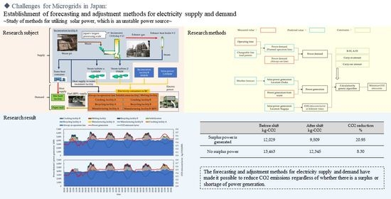
• Developed a prediction method by analyzing the power data of operation plan line, always in operation line, waste power generation, and solar power generation. For solar power generation, the average error was 125.3 kW by predicting the amount of solar radiation based on the weather forecast.
• Calculated the CO₂ emission factor by time of the day from the data of power company A analysis. This study also developed a method to predict the CO₂ emission factor by time of the day with a prediction accuracy of 0.81 by predicting the solar power generation amount in power company A.

Results showed that by formulating an operation plan for the operation plan line using CO₂ emission factor by time of the day and a method for predicting power load and power generation, CO₂ emissions could be reduced by 20.95% in weeks with high solar power generation and by 8.30% in weeks with low high solar power generation.

The limitation of this study was that the actual operation plan could not be acquired (this study only estimated it using the power data due to company confidentiality). Furthermore, personnel constraints were not considered in the proposed operation plan.

When constructing an operation plan of a similar power generation facility with the purpose of CO₂ emissions reduction, it is necessary to accurately predict the following three parameters: (1) power generation, (2) power demand, and (3) CO₂ emission factor. Thus, while the prediction method developed in this study can be used as a benchmark, future works analyzing other facilities must employ the actual parameters from the specific plants. Additionally, the target power load facilities in this study are limited to industrial facilities in the industrial sector. Actual users in the region include residential and commercial facilities, hospitals, and public facilities. The findings of this study can be used to establish a forecasting method for waste treatment facilities and to plan electricity use that minimizes CO₂ emissions as a region.

References

1. Bunme, P.; Yamamoto, S.; Shiota, A.; Mitani, Y. GIS-Based Distribution System Planning for New PV Installations. Energies 2021, 14, 3790. [Google Scholar] [CrossRef]
2. Ahmed, W.; Ahmed Sheikh, J.; Parvez Mahmud, A. Impact of PV System Tracking on Energy Production and Climate Change. Energies 2021, 14, 5348. [Google Scholar] [CrossRef]
3. Japan’s Energy Problems. Available online: https://www.enecho.meti.go.jp/about/special/johoteikyo/energyissue2020_1.html (accessed on 30 September 2021). (In Japanese).
4. Agency for Natural Resources and Energy; Ministry of Economy. Trade and Industry. Available online: https://www.enecho.meti.go.jp/statistics/total_energy/pdf/gaiyou2019fyr.pdf (accessed on 1 October 2021). (In Japanese)
5. Ministry of the Environment . Available online: https://www.env.go.jp/earth/ondanka/ghg-mrv/emissions/results/JNGI2019_sankou.pdf (accessed on 1 October 2021). (In Japanese)
6. Akita, N.; Ohe, Y.; Araki, S.; Yokohari, M.; Terada, T.; Bolthouse, J. Managing Conflicts with Local Communities over the Introduction of Renewable Energy: The Solar-Rush Experience in Japan. Land 2020, 9, 290. [Google Scholar] [CrossRef]
7. Castilho, C.D.; Torres, J.P.; Fernandes, C.A.; Lameirinhas, R.A. Study on the Implementation of a Solar Photovoltaic System with Self-Consumption in an Educational Building. Energies 2021, 14, 2214. [Google Scholar] [CrossRef]
8. Nishikawa, S.; Nakao, A.; Yamamoto, S.; Yamamoto, Y.; Nakakubo, T.; Yoshida, N. Effects of extended heat recovery and waste collection on power generation efficiency and business feasibility for a high-efficient waste power generation plant with reserve capacity. J. Jpn. Soc. Civ. Eng. Ser. G 2017, 73, II_379–II_390. [Google Scholar] [CrossRef]
9. Greenhouse Gas Protocol. Available online: https://ghgprotocol.org/standards/scope-3-standard (accessed on 7 January 2021). (In Japanese).
10. Ministry of the Environment. Available online: https://ghg-santeikohyo.env.go.jp/files/calc/itiran_2020_rev.pdf (accessed on 31 August 2021). (In Japanese)
11. Miike, H.; Nanno, I. Light and Shadow of the Solar Power Generation: Consideration of Local Climate and Culture of Calendar-Based on the Analysis of a Record of 10 Years Photovoltaic Generation. Time Stud. 2019, 10, 1–18. [Google Scholar]
12. Yamada, H.; Ikki, O. National Survey Report of PV Power Applications in Japan 2012. In International Energy Agency Co-operative Programme on Photovoltaic Power Systems; IEA & New Energy and Industrial Technology Development Organization (NEDO): Kawasaki, Japan, 2013. [Google Scholar]
13. Kyushu Electric Power Transmission and Distribution Co., Inc. Available online: https://www.kyuden.co.jp/td_renewable-energy_purchase_control.html (accessed on 2 September 2021). (In Japanese).
14. Oozeki, O. National Institute of Advanced Industrial Science and Technology . Available online: https://unit.aist.go.jp/rpd-envene/PV/ja/results/2010/20Ozeki.pdf (accessed on 1 October 2021). (In Japanese).
15. Goto, I.; Higashi, H. Electric Load Forecasting System for Electricity Retailers. SEI Tech. Rev. 2015, 187, 60–65. [Google Scholar]
16. TEPCO Energy Partner, Inc. Peak Shift Plan. Available online: https://www.tepco.co.jp/ep/private/plan2/old06.html (accessed on 1 October 2021). (In Japanese).
17. Morita, H.; Ishida, C.; Onishi, A.; Kawahara, S.; Imura, H.; Kato, H. An Effect of a “Demand Response” Power Model to Energy Saving Behavior and Energy Consumption. Proc. JSCE 2015, 71, I357–I368. [Google Scholar]
18. TEPCO Ventures, Inc. Available online: https://www.tepcoventures.co.jp/flexbee/demand_response (accessed on 1 October 2021). (In Japanese).
19. International Renewable Energy Agency. Planning for the Renewable Future Long-Term Modelling and Tools to Expand Variable Renewable Power in Emerging Economies; International Renewable Energy Agency: Abu Dhabi, United Arab Emirates, 2017; pp. 9–111. [Google Scholar]
20. Agency for Natural Resources and Energy; Ministry of Economy. Trade and Industry. Available online: https://www.meti.go.jp/shingikai/enecho/denryoku_gas/genshiryoku/pdf/021_03_00.pdf (accessed on 1 October 2021). (In Japanese)
21. Bureau of environment Tokyo Metropolitan Government. Available online: https://www.kankyo.metro.tokyo.lg.jp/data/publications/resource/industrial_waste/industrial_waste.files/P13-P25.pdf (accessed on 1 September 2021). (In Japanese)
22. Mie Prefectural Government. Available online: https://www.oshigoto.pref.mie.lg.jp/kigyonavi/1504 (accessed on 2 September 2021). (In Japanese)
23. Kansai Bureau of Economy. Trade and Industry. Available online: https://www.kansai.meti.go.jp/3-6kankyo/R3fy/03_mie.pdf (accessed on 2 September 2021). (In Japanese)
24. Sanki Engineering Co., Ltd. Available online: https://www.sanki.co.jp/product/thc/outline/ (accessed on 30 September 2021). (In Japanese).
25. Fukuma, Y.; Fujikawa, H.; Matsuda, Y.; Watase, M.; Matsuto, T. Estimating Heat Generation and Heating Values by Exhaust Gas Composition for a Municipal Solid Waste Incinerator. J. Jpn. Soc. Mater. Cycles Waste Manag. 2018, 29, 8–19. [Google Scholar] [CrossRef] [Green Version]
26. Horisaki, S. Demonstration Experiment of Photovoltaic Power Generation Prediction Method Using Weather Data. Unisys Technol. Rev. 2017, 134, 47–56. [Google Scholar]
27. Ministry of the Environment. Available online: https://ghg-santeikohyo.env.go.jp/files/calc/cm_ec_R03/full.pdf (accessed on 1 October 2021). (In Japanese)
Figure 1. Changes in Japan’s Energy Mix [3,4].
Applsci 11 10747 g001
Figure 2. Material flow in RC.
Applsci 11 10747 g002
Figure 3. RC energy flow.
Applsci 11 10747 g003
Figure 4. Energy balance.
Applsci 11 10747 g004
Figure 5. Image of operation shift.
Applsci 11 10747 g005
Figure 6. Operation planning line (crushing facility A) load pattern.
Applsci 11 10747 g006
Figure 7. Load pattern of continuous operation line (a new water treatment facility).
Applsci 11 10747 g007
Figure 8. Amount of power generated by waste power generation facilities.
Applsci 11 10747 g008
Figure 9. Amount of solar power generation by weather.
Applsci 11 10747 g009
Figure 10. Operation planning line (Manufacturing facility A) load pattern.
Applsci 11 10747 g010
Figure 11. Load pattern of continuous operation line (Roasting pretreatment facility).
Applsci 11 10747 g011
Figure 12. Incineration facility B.
Applsci 11 10747 g012
Figure 13. Comparison of solar radiation prediction methods.
Applsci 11 10747 g013
Figure 14. Power generation record of electric power company A.
Applsci 11 10747 g014
Figure 15. Relationship between solar power generation and CO2 emission factor.
Applsci 11 10747 g015
Figure 16. Relationship between the amount of crushing facility A and solidification facility input and operating time.
Applsci 11 10747 g016
Figure 17. Relationship between the carry-in/out volume and operating time of facilities other than crushing facility A and solidification facility.
Applsci 11 10747 g017
Figure 18. Relationship between operating time and weekly operating power.
Applsci 11 10747 g018
Figure 19. Relationship between operating time and weekly operating power.
Applsci 11 10747 g019
Figure 20. The logic for calculating planned operating values.
Applsci 11 10747 g020
Figure 21. Results of weekly operational shifts where surplus power is generated.
Applsci 11 10747 g021
Figure 22. Weekly operation shift results with no surplus power.
Applsci 11 10747 g022
Figure 23. Comparison of solar power generation and CO2 emission factor made one week and two days in advance.
Applsci 11 10747 g023