Feasibility of Acoustic Print Head Monitoring for Binder Jetting Processes with Artificial Neural Networks

Abstract

The clogging of piezoelectric nozzles is a typical problem in various additive binder jetting processes, such as the manufacturing of casting molds. This work aims at print head monitoring in these binder jetting processes. The structure-born noise of piezoelectric print modules is analyzed with an Artificial Neural Network to classify whether the nozzles are functional or clogged. The acoustic data are studied in the frequency domain and utilized as input for an Artificial Neural Network. We found that it is possible to successfully classify individual nozzles well enough to implement a print head monitoring, which automatically determines whether the print head needs maintenance.

1. Introduction

Additively manufactured (AM) components are built layer by layer, which enables the production of products of high complexity as well as filigree, rigid, and high-strength structures. Advantages of this process, such as almost unlimited design freedom and tool-free production, allow for a wide variety of applications in many fields [1]. Innovative foundry manufacturers discovered the benefits of additive manufacturing early on. Additively manufactured patterns, molds, and cores have several advantages, including improved part consolidation, material efficiency and on demand production [2]. Therefore, they are now being increasingly used and have become mainstream in this industry. As the actual component is produced using a conventional casting process, this type of additive manufacturing is referred to as indirect additive manufacturing [3].

Additive manufacturing of molds and cores in the foundry industry can be based on an organic cold resin system [4]. Another possibility is the use of an inorganic binder system [3]. In this case, an inorganic binder based on water glass is applied to the sand bed. Compared to organic binders, inorganically-bound cores and molds have various advantages [5]. For example, there are no emissions during core production, a significant reduction in emissions during casting, no organic condensate adhesion to the casting, and improved material properties. In addition, the economics of the casting process are improved due to reduced maintenance of casting tools and reduced air treatment [6].

One challenge in 3D printing with an inorganic molding material system is part quality. The possible drying of individual nozzles on the 3D printer’s print head can result in unconnected areas in the part [7], which have lower strength due to the lack of binder. Inorganic binder systems need thermally induced curing [1]. However, inorganic core binders can also be activated by CO₂ [8]. Therefore, the binder in the nozzle can solidify if it is in contact with CO₂ without cleaning it regularly. According to Günther et al., another reason for defective nozzles is buildup on the print head, such as sand grains or misdirected drops [9].

To counteract the problem of defective nozzles, the condition of print heads is usually checked manually before each print job by printing a test pattern on a pH indicator paper. If the quality of the print head falls below a defined threshold, various cleaning processes can be used to restore the functionality of the nozzles. This procedure allows the condition of the nozzles to be checked and, if necessary, improved before the printing process begins. Another possibility is the continuous optical control of each layer as proposed by Günther et al. [9]. Defective nozzles can be detected by lines without binder in the individual layers.

This article aims at a feasibility study of acoustic print head monitoring. Modal analysis is a popular way to determine the elastic parameters of materials [10,11]. However, the monitoring of industrial manufacturing processes is researched in numerous articles as well [12,13].

In this article, an acoustic print head analysis is implemented, instead of manual control by means of a test print. This acoustic analysis can be automated easily and has the potential for online monitoring. In a first step, the acoustic data must be recorded by attaching a suitable sensor system for monitoring the print head. In addition, a suitable evaluation methodology must be developed that searches for acoustic patterns in the signal and uses these to draw conclusions about the condition of the nozzles. This evaluation will be performed with Artificial Neural Networks (ANN). ANNs and machine learning have been utilized to evaluate acoustic emissions and structure born noise in an industrial environment for predictive maintenance in numerous articles [12,14], however there is no study on the analysis of piezo print heads.

2. Materials and Methods

2.1. Binder Jetting Equipment

The experiments are performed on a VX500 sand binder jetting system (Voxeljet AG, Friedberg, Germany). This printer is used for the production of inorganically-bound sand molds and sand cores. As the print head was of primary importance for the tests and investigations of this article, the print head structure and print head cleaning of the print head will now be explained in more detail below.

The print head is supplied with printing and cleaning fluid by the system’s fluid system. The fluid system also collects the waste fluid produced during the printing process. There are a total of six Spectra SL-128 AA, FUJIFILM Dimatix printing modules inside the print head, with each printing module containing 128 piezoelectric nozzles. In total, there are 768 individually controllable piezoelectric nozzles in the print head.

To ensure print quality, the print head must be maintained and cooled in the cleaning station before and during the printing process. The cleaning station contains a foam roller that is moistened from the fluid system. In addition, a pressure roller pushes binder residue out of the cleaning roller, which is intended to prevent degradation of the foam by the binder [15]. In idle mode, the print head is on the capping station. Here, a damp sponge is pressed against the print modules from below, which protects them from drying out. According to the authors of [15], a standard print head cleaning consists of a 0.5 s purge operation, a double roller pass, and a free spraying of the modules with 10,000 shots. During the so-called purge operation, the negative pressure supply is reversed for a short period of time and the fluid tank is pressurized with positive pressure. This causes fluid to flow through all nozzles. The overpressure is intended to purge clogged nozzles. The second part of the standard print head cleaning process, the roller pass, removes fluid droplets that have formed on the underside of the print head. During the spraying process, all 768 nozzles are activated for one second, which is supposed to ensure a stable condition of the nozzles.

2.2. Measurement System

A sensor of type 8702B500 from Kistler (Kistler Instrumente GmbH, Munich, Germany) was used for acceleration measurements. With this type of sensor, the signal is generated by a shear ceramic measuring device and converted into a voltage signal by evaluation electronics integrated in the sensor. The sensor is characterized by low lateral sensitivity and low sensitivity to base strain. The sensor has a resonant frequency of 54 kHz and has a measurement range of up to ±500 g [16]. The supply voltage as well as the signal processing was provided by a RogaDAQ 2, which is recognized as a standard sound device by a PC. Manufacturer of this portable high performance data acquisition device is ROGA-Instruments (Nentershausen, Germany). The RogaDAQ 2 supports measurements from 0 Hz to 20 kHz with an input limit of ±5 volts.

In principle, several different options are available for mounting the accelerometer on the print head. Kistler offers magnetic mounting adapters, adhesive mounting adapters, adhesive axles, or mounting bolts as mounting options. Due to the high frequencies to be expected in the signal, a mounting bolt was selected for fastening the sensor, which represents the stiffest of all connection options [17]. Figure 1 depicts the mounting of the sensor on the print head. Highlighted are the accelerometer (1), the threaded nut for position assurance (2), the threaded nut for clamping (3), the spacer plate (4), and the surrounding steel plate (5).

2.3. Data Acquisition and Evaluation

When recording the test data, several measurements were combined into one audio signal. This simplified the recording process, as it was not necessary to store each signal individually. The piezoelectric frequency of the print head can theoretically be set to a value of 30 kHz, but was kept constant at 10 kHz for all test series, as this is the usual printing frequency.

Table 1. Recording and print head settings for the experiments in this article.

Parameter	Symbol	Value
Frequency of the piezoelectric actuator	fPiezo	10 kHz
Number of nozzle shots	nshots	10,000
Sample rate of the measuring system	fsample	48 kHz
Number of samples in the signal	nsample	40,000

summarizes the most important parameters of the print head and the data acquisition.

We attempted to determine whether a nozzle was functional or not on the basis of the recorded experimental vibration data. To determine the nozzle condition, the ejection of a droplet from the nozzle was utilized as the evaluation criterion. This means that if a droplet ejection was visible, the nozzle was classified as working correctly. If no droplet ejection could be detected when the nozzle was actuated, the nozzle was considered to be faulty (clogged). The vibration data was recorded on four different days to study time-dependent influences. In addition, the times of the recordings were chosen such that the level of background noise was as low as possible in order to achieve a minimum of background noise. Therefore, the measurement recordings took place before 8:00 a.m. or after 5:00 p.m.

The tested nozzle was located approximately in the center of the print head and represents the 70th nozzle in the fourth module of the print head. To check the nozzle condition, a glass mirror was used, which was located below the piezoelectric modules during activation. After each nozzle activation, it was visually checked whether there was a drop on the mirror. If a drop was visible on the mirror, the mirror was cleaned and placed under the print head again for the next measurement. A total of 480 individual measurements were recorded in the course of this series of tests, which were recorded at four different dates, each with 120 individual measurements. At each measurement date, the measurements were again split into four data blocks. This means that in one day two data blocks with a functional nozzle and two data blocks with a clogged nozzle were recorded, each with 30 individual measurements of a nozzle actuation. The sequence of a data block of 30 individual measurements can be seen in the following figure.

Figure 2 shows the recording of a data block with 30 nozzle shots. At the beginning, all nozzles of the print head were always cleaned. A standard cleaning and a purge process were carried out. Then, the measuring position was approached and the corresponding nozzle condition was checked. If the visual inspection showed that the state of the nozzle was as desired (functional or clogged), the nozzle could be triggered again. If the state was not as desired, the print head was cleaned to achieve a functional nozzle or the experiments were paused for 5 min to achieve a clogged nozzle. Thirty nozzle shots form a data block, with a consistent nozzle state in each block.

2.4. Reference Network and Training

The ANN used for the evaluation of the acoustic data is built with a four-layer feedforward network which uses tansig activation functions (specified in Equation (1)) for the hidden layers and the softmax function (specified in Eqaution (2)) for the output layer. In general, such a network is well suited for pattern recognition, where different input vectors are classified into given target categories [18]. We use supervised ANNs in contrast to unsupervised ANNs to ensure the best possible success rate in the classification problem. The additional experimental effort for labeling the training data in an industrial application will be small compared to the repeated manual effort of monitoring the print head with a test pattern. The Fast Fourier Transformation (FFT) of the recorded signal is utilized as input data. After specifying input and target values, the training function for the ANN was determined. In principle, Matlab provides a large number of different training functions, which can be selected depending on the application and the available computing power. A detailed overview can be found under [19]. The algorithm trainscg was selected, where scg is the abbreviation for Scaled Conjugate Gradient Backpropagation. This algorithm is used by default in Matlab for pattern recognition problems and is also well suited for large networks, according to the work in [20], as it is very efficient. As the number of input and output neurons was already specified by the input and target matrices, only the size and number of hidden layers had to be specified to fully define the network size. All relevant parameters can be found in

Table 2. Important parameters of the reference-ANN utilized for the data evaluation.

Parameter	Value/Setting
Neurons—input layer	20,000
Neurons—hidden layer 1	100
Neurons—hidden layer 2	60
Neurons—output layer	2
Activation function—hidden layers	tansig
Transfer function—output layer	softmax
Error measure	mean squared error (mse)
Training function	Scaled Conjugate Gradient Backpropagation
Early Stopping	80 epochs

.

The available input data were divided into training data, validation data, and test data. The distribution was random; 70% of the data was used for training, 15% for validation, and the remaining 15% as test data. The training data are used for the actual training. Based on these data, the gradients are calculated and the individual weights are updated at each iteration. In contrast, the validation data are used to prevent overfitting. An overfitted ANN is overtrained on the given training data, reducing the prediction accuracy for further unknown data sets which were not part of the training data set. To prevent this, so-called early stopping is used. If the calculated error between the target and initial values of the network exceeds the error limit for the validation data over several iterations and, at the same time, the error of the training data continues to decrease, this is an indicator of so-called overfitting [20]. By specifying a maximum number of training epochs, an early stop of the training is enforced. Finally, the weights are assigned the values that produced the minimum error in the validation data set, thus preventing overfitting.

The FFT of the respective signal is used as input values of the ANN. In advance, a short overview of the most important settings and parameters of the used reference networks is given in Table 2. These parameters will be optimized in the next section.

$$\mathrm{tansig}\left(\mathrm{N}\right)=\frac{2}{1+exp(-2N)}-1$$

(1)

$$\mathrm{softmax}\left(\mathrm{N}\right)=\frac{exp\left(N\right)}{\sum (exp(N\left)\right)}$$

(2)

3. Results and Discussion

3.1. Analysis in the Time Domain vs. in the Frequency Domain

Before creating an ANN for the data evaluation, we attempted to find analytical correlations within the data. In a first step, the acoustic signals of the clogged and correctly operating nozzle are compared in the time domain.

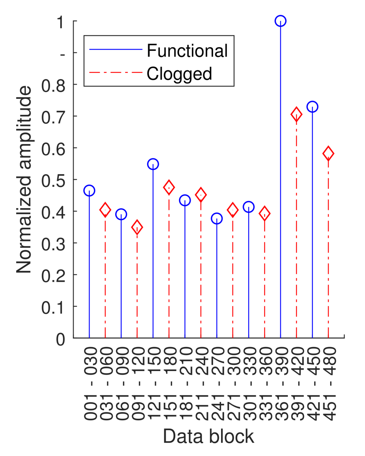
Figure 3 shows the mean values of the amplitudes of the recorded signals, which are normalized to the highest amplitude mean value occurring. Thirty data points were grouped in each case. In Figure 3, the state of the nozzle was set to the same value within these 30 data points (functional or clogged). The amplitude average of the functional nozzles tends to be higher than the amplitude average of the clogged nozzles. One possible explanation would be that the sound propagation is damped due to a clogged nozzle, which would be reflected accordingly in a lower amplitude. However, the amplitudes have a high scatter from data block to data block compared to this amplitude difference between clogged and functional nozzles.

In addition to the observations of the amplitude averages in the time domain, the signals will be analyzed in the frequency domain in the following. For this purpose, a FFT of the signals was performed in Matlab. The resulting frequencies are calculated with the sample rate and the associated number of samples.

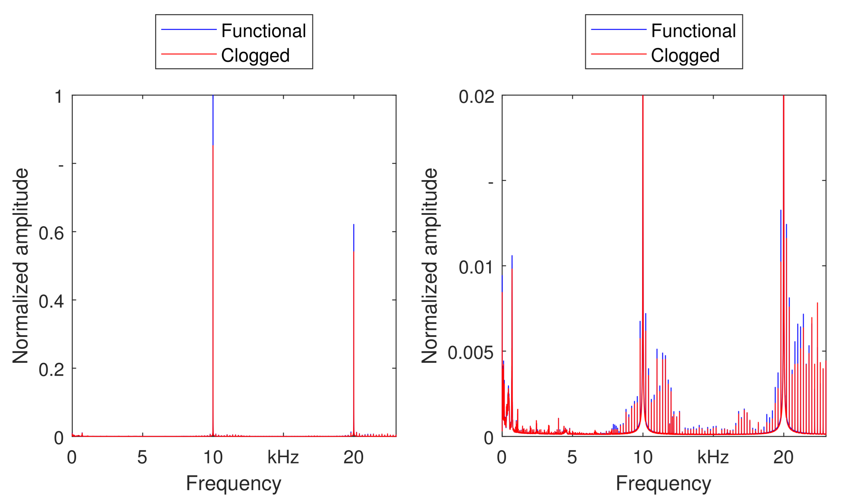
Figure 4 shows that the maximum is at a frequency of 10 kHz, which corresponds to the frequency settings of the piezoelectric actuators. In addition, the first harmonic can be seen at twice the fundamental frequency of the piezoelectric actuators. The hypothesis is that the amplitudes at a frequency of 10 kHz are higher in the frequency range for a functional nozzle than those of a clogged nozzle. While Figure 4 (left) shows the complete signal in the frequency domain, Figure 4 (right) shows a zoom representation of the previous figure, which also allows the analysis of lower amplitude values. Functional nozzles (blue) show a higher amplitude than clogged nozzles (red) not only at a frequency of 10 kHz and 20 kHz, but also in the surrounding frequency ranges. In the low-frequency range from 0 to 7.5 kHz, no difference in amplitude can be found between functional and clogged nozzles. This also seems quite plausible, as in this range it is mainly background noise that is independent of the nozzle condition. Furthermore, no shift in the frequency peaks can be detected. In summary, it can be stated that in both the time and frequency domain, the evaluated amplitudes of a functional nozzle tend to be higher than the amplitudes of a clogged nozzle. However, as the observations are mean amplitudes and there is significant scatter between the data blocks, no clear correlation for the classification of the nozzle condition can be concluded on the basis of these analytic investigations. For this purpose, an ANN will be set up in the next section and used for noise pattern analysis.

3.2. Evaluation with the Reference Network in the Frequency Domain

As described above, the data were recorded on four different dates. A k-fold cross-validation is applied for the following evaluation. This cross-validation represents a common technique for evaluating a model in machine learning. Here, the input data are partitioned and multiple models are trained with the partial data sets. The remaining part of the respective input data serves as a test data set. The overall success rate is calculated from the average of the individual success rates. This procedure prevents overfitting during training [21]. With respect to the present use case, this means that four networks are built up, each of which is based on the sound data of three different measurement dates, while the forth is used for testing.

Table 3. Correct classifications for each measurement date based on the training with data acquired on the remaining three dates.

Date	Success Rate	(Min/Max)
Date 1	64.6%	(Min: 53.4%, Max: 85.6%)
Date 2	72.2%	(Min: 61.5%, Max: 82.8%)
Date 3	49.4%	(Min: 48.3%, Max: 51.7%)
Date 4	65.7%	(Min: 57.0%, Max: 71.1%)
Average	63.0%

gives an overview of the success rate achieved in the classification of the nozzle state with the reference network.

Table 3 shows that the nozzle condition was correctly determined in 63% of the classifications by the network. The success rate obtained is the average of all four measurement dates. The success rate of each individual measurement date in turn represents an average value, which refers to ten separately trained ANNs. In addition to these mean values, the minimum and maximum of each measurement date are also shown in Table 3. Particularly noticeable is measurement date 3, where only 49.4% of all nozzle states can be correctly classified. The success rate of the other three measurement dates, on the other hand, is significantly higher. Therefore, for a more in-depth analysis, a confusion matrix of the test data from measurement date 3 is necessary. As the difference between minimum and maximum is small, the ANN with the lowest success rate of all ten trained networks is utilized as a worst case study.

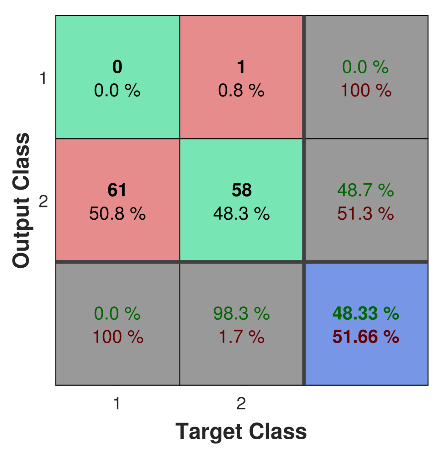
Figure 5 shows the confusion matrix of measurement date 3. A confusion matrix allows us to represent the results of a classification problem more comprehensively. The columns of the matrix represent the given target class, whereas the rows represent the output class determined from the ANN. Target class 1 represents a functional nozzle and Target class 2 represents a clogged nozzle. The correctly classified nozzle states can be taken from the main diagonal of the matrix. Of the total 120 nozzle shots, 58 were correctly identified, which is consistent with the success rate of the minimum from Table 3. The advantage of a confusion matrix is primarily the visualization of the misclassified nozzle states, which distinguishes between false positive and false negative errors [22]. The lower left red box of the matrix shows the number of nozzles that were functional during the experiments but were classified as clogged by the network. The upper right red field, on the other hand, shows the number of nozzles that were clogged during the experiments but were incorrectly detected as functional by the network. By dividing the falsely classified nozzles into false positive and false negative errors, it becomes clear that the network evaluates almost all nozzles as clogged, regardless of the actual nozzle condition. All 61 nozzles that were “functional” when the sound was recorded are misclassified.

The reason for the large number of false evaluations could be the level of the amplitudes in the time domain. The amplitude averages of the acoustic signals of all functional nozzles of measurement date 3 (measurements 241–270 and measurements 301–330) are lowest and tend to be in the range of the clogged nozzles. Presumably, the ANN reacts to the low amplitude values, which accordingly results in the large number of false evaluations.

In summary, information of the nozzle state is present in the signal, as overall the success rate of 63.0% is above the limit of 50%, which would statistically result from a binary classification problem assuming a uniform distribution by randomly assigning the nozzle state. However, the achieved success rate is too low for a technically reasonable application. In the next section, the preprocessing of the data and the network itself will be optimized to improve the number of correct classifications.

3.3. Normalizing the Signal Amplitude

By considering the amplitude averages in the architecture of the signal processing, the different findings from the previous section are combined. By normalizing the amplitudes in the time domain with the maximum amplitude in a preprocessing step, an increase of the success rate to 70.4% can be achieved. Detailed results are presented in

Table 4. Classification success rates with the reference network after normalizing the acoustic signals in a preprocessing step in the time domain.

Date	Success Rate	(Min/Max)
Date 1	56.3%	(Min: 46.6%, Max: 64.4%)
Date 2	84.3%	(Min: 79.5%, Max: 88.5%)
Date 3	56.3%	(Min: 50.8%, Max: 62.5%)
Date 4	84.8%	(Min: 70.2%, Max: 94.2%)
Average	70.4%

. All settings and network parameters were selected analogously to the original reference network. It is also worth taking a closer look at the success rates of the individual measurement dates. Due to normalization, the success rates of measurement dates 2, 3, and 4 increase, whereas measurement date 1 achieves a lower success rate.

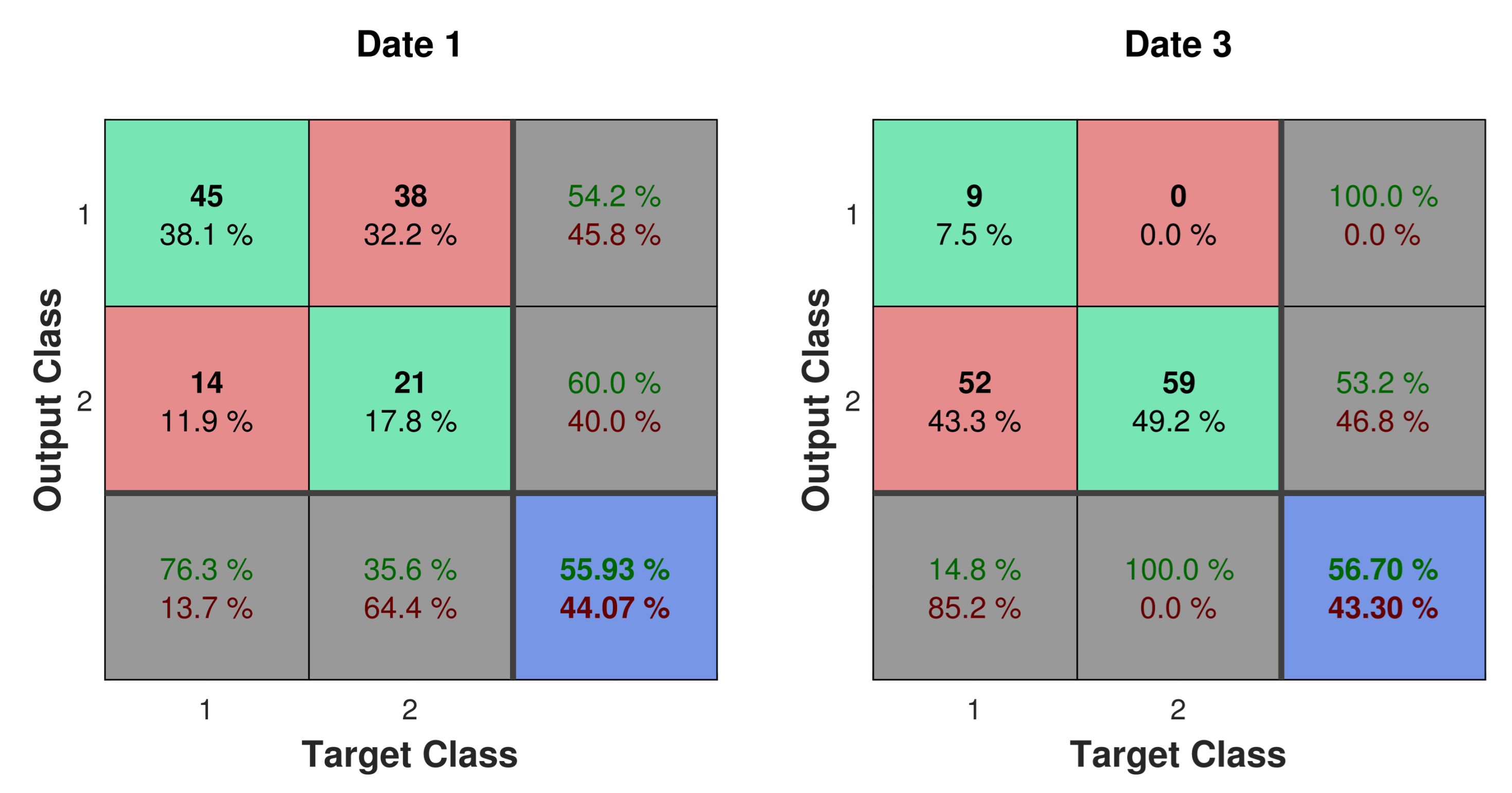
Although measurement dates 1 and 3 have a comparable overall success rate, a closer look at the confusion matrices in Figure 6 reveals differences. Analogous to Figure 5, the number of functional nozzles is classified with state 1 and the number of clogged nozzles with state 2. When comparing the two measurement dates, the ANN assigns a majority of the output to class 1 for measurement date 1 and a majority of the output to class 2 for measurement date 3, irrespective of the actual nozzle state. In purely theoretical terms, the distribution of each measurement date should be balanced for an ideal success rate, as half of all test data represents a functional nozzle state and the other half represents a clogged nozzle state. In addition, the influence of the above-described normalization of the amplitude in the time domain is particularly interesting. At measurement date 3, when compared with the original condition (see Figure 5), 7.5% of all functional nozzles can be correctly classified as a result of the normalization. Without this modification, not a single functional nozzle could be recognized as such. However, the ANN still assigns the state clogged to more than 90% of the input values. In contrast, the success rate of the first measurement date is much more balanced compared to the third measurement date. Although the ANN increasingly assigns the state 1 (functional), 17.8% of all clogged nozzles can also be detected. Furthermore, in contrast to measurement date 3, both false positive and false negative errors occur.

In summary, it can be stated that the performed normalization leads to an improvement of the overall success rate. The achieved 70.4% are in a range which is interesting from a technical point of view. However, the measurement date still influences the success rates considerably.

3.4. Influence of Sample Time

This section focuses on the optimization of the recording time, which may improve the success rate, as well as the technical feasibility. As all nozzles must be tested one after the other for their functionality when checking the complete print head, the sampling time is an important parameter for the technical feasibility. With 768 individual nozzles, it is advantageous to reduce the recording time per nozzle as far as possible. The reduction of the recording time t_recording affects the number of samples n_sample available for the evaluation at a constant sample rate f_s, which becomes clear from Equation (3).

$$n_{sample}=t_{recording}·f_s$$

(3)

Equation (3) shows that there is a linear relationship between sample number and recording time. The number of samples available for the evaluation in turn affects the sampling interval $\mathsf{\Delta }f$ of the discrete Fourier transform, which is used as input for the ANN. The sampling interval can be determined from the sample rate f_sample and the sample number n_Sample. With Equation (3), the sampling interval $\mathsf{\Delta }f$ is calculated according to

$$\mathsf{\Delta }f=\frac{f_s}{n_{sample}}=\frac{1}{t_{recording}}$$

(4)

Equation (4) shows that the reduction of the recording time causes an increase of the sampling interval. This influence on the success rate will be examined in the following. The reduced recording time is simulated by cutting of the respective signal. Starting from the maximum recording duration, which corresponds to a sample number of 40,000, the sample number is continuously reduced and the success rate is determined. The architecture of the ANN is analogous to the previous experiments. In addition, the amplitude of the input values in the time domain are again normalized.

As the evaluation of parameter influences is based on the available test data, these can now no longer be regarded as independent. In order to ensure the general validity of the success rate nevertheless, the principle of data splitting is utilized again. For this purpose, the test data sets used in the cross-validation are divided into two parts by numbering the totality of all test data and combining all even or all odd measurement values into one test data level each. The first part of the data (1st stage) is used to determine the success rate and, on the basis of this, to evaluate the influence of the parameters. To ensure that the optimization is not specifically tailored to the first part of the test data set, the success rate achieved is then checked with the independent part: the second stage of the data. 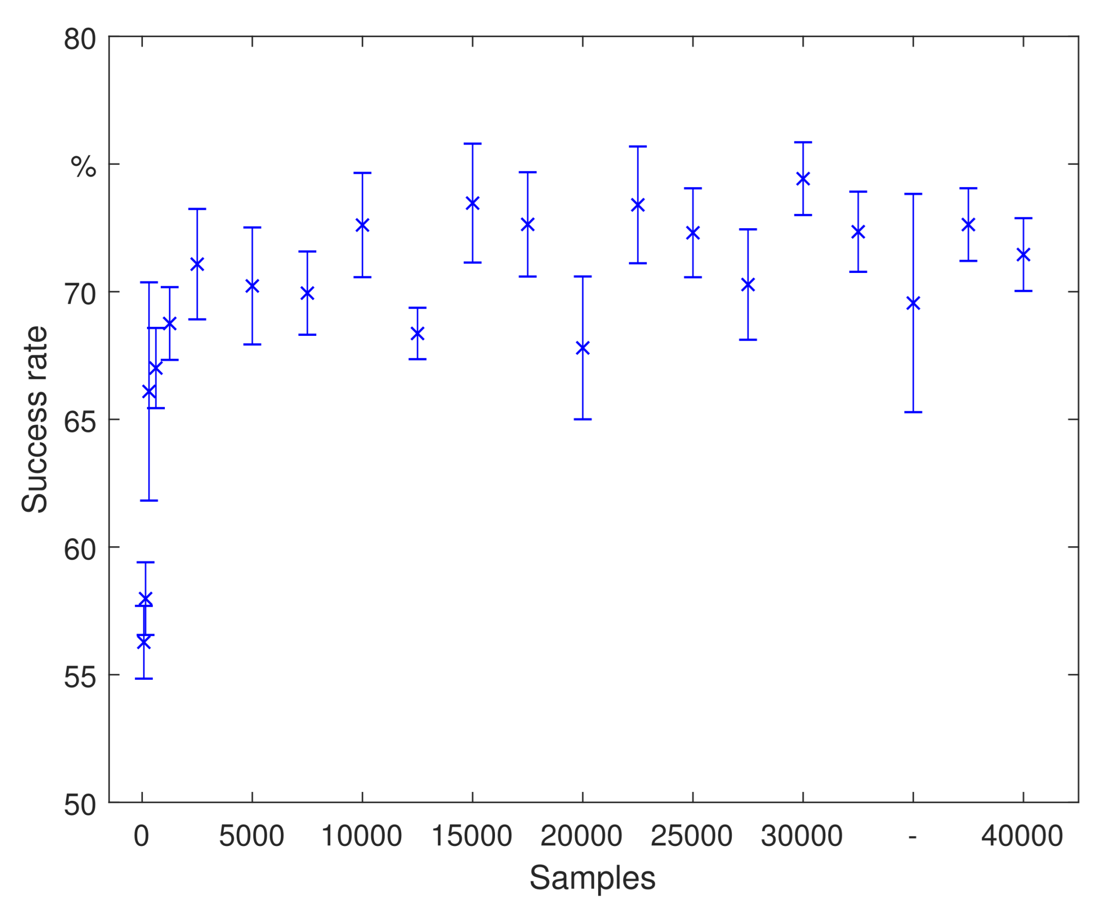Figure 7 shows the independent results for the variation of the number of samples. Please note that up to 5000 samples five different networks were utilized, while 20 networks were utilized from 5000–40,000 samples to increase to validity of the results.

The mean values are marked by a blue x, additionally the standard deviation is given for each sample size. Particularly striking is the steep drop in the success rate below a sample number of 2500. Below this limit, the reduction of the sample number and the associated increase of the sampling interval seems to make it very difficult for the ANN to recognize the nozzle state. At a sample number of 100, the success rate is only 56%. Figure 7 shows that an increase in the sample number does not necessarily lead to an increase in the success rate.

Based on these considerations, the optimization potential can now be evaluated by varying the number of samples. The analysis of Figure 7 shows that the maximum success rate of 74% is achieved with a sample number of 30,000. Compared to the original setting with a sample number of 40,000, this corresponds to an improvement of 3.6%. In order to test the statistical significance of this improvement, a z-test was performed in Matlab which rejected the hypothesis that the results at 30,000 samples and 40,000 samples originate from the same distribution at a 4% significance level. This indicates that the improvement is significant compared to the scatter.

From a production engineering point of view, it is also of interest how long the classification process takes for the whole print head with 768 nozzles, as the machine is not able to produce during classification. 30,000 samples correspond to 0.83 s for each tested nozzle or 480 s for the whole print head. Therefore, in the following a second sample number will be proposed, which also takes the necessary sampling time into account. It may be necessary to maximize the classification success or to save time in an industrial application, depending on the specific printing geometry. Therefore, a compromise must be found at which the number of samples can be kept as low as possible, but at the same time the success rate can be kept sufficiently high. According to Figure 7, it seems reasonable to define this mark at 10,000 samples. The success rate here has a value of about 72%. A z-test has failed to reject the hypothesis that the results at 10,000 samples and 40,000 samples originate from the same distribution up to a 35% significance level, which indicates similar success rates. Furthermore, the success rate is already in an approximately stable range, which has a safe distance to the lower boundary of 2500 samples. By setting the limit at a sample number of 10,000, it is possible to reduce the recording time (testing time for the whole print head: 160 s) without having to accept a deterioration in the success rate of the ANN.

3.5. Optimization of Network Architecture and Parameters

In this section, the parameters and the layer sizes of the ANN will be chosen systematically. First, the training function and the error measure will be varied for 10,000 samples to choose the best option. We tested multiple training functions, which are available in Matlab. The resulting success rates are presented in

Table 5. Success rate depending on the training function of the ANN.

Training Function	Success Rate
trainscg (Scaled conjugate gradient backpropagation)	72.7%
traincgb (Conjugate gradient backpropagation with Powell–Beale restarts)	72.6%
traincgf (Conjugate gradient backpropagation with Fletcher–Reeves updates)	69.5%
traincgp (Conjugate gradient backpropagation with Polak–Ribiere updates)	70.8%
traingd (Gradient descent backpropagation)	69.5%
traingda (Gradient descent with adaptive lr backpropagation)	69.1%
traingdm (Gradient descent with momentum)	68.5%
traingdx (Gradient descent with momentum and adaptive lr backpropagation)	69.2%
trainoss (One step secant backpropagation)	71.3%

. The training function of the reference network, already offers the best success rate. Therefore, no change is necessary. Analogously, multiple error functions for the training with the trainscg function have been tested (results in

Table 6. Success rate depending on the error measure in the training of the ANN.

Error Measure	Success Rate
mse (Mean squared error performance function)	72.7%
mae (Mean absolute error performance function)	67.6%
crossentropy (Cross-entropy performance)	71.9%
sae (Sum absolute error performance function)	71.6%
sse (Sum squared error performance function)	72.5%

). The maximum success rate was achieved with the mean square error measure, which was already implemented in the reference network.

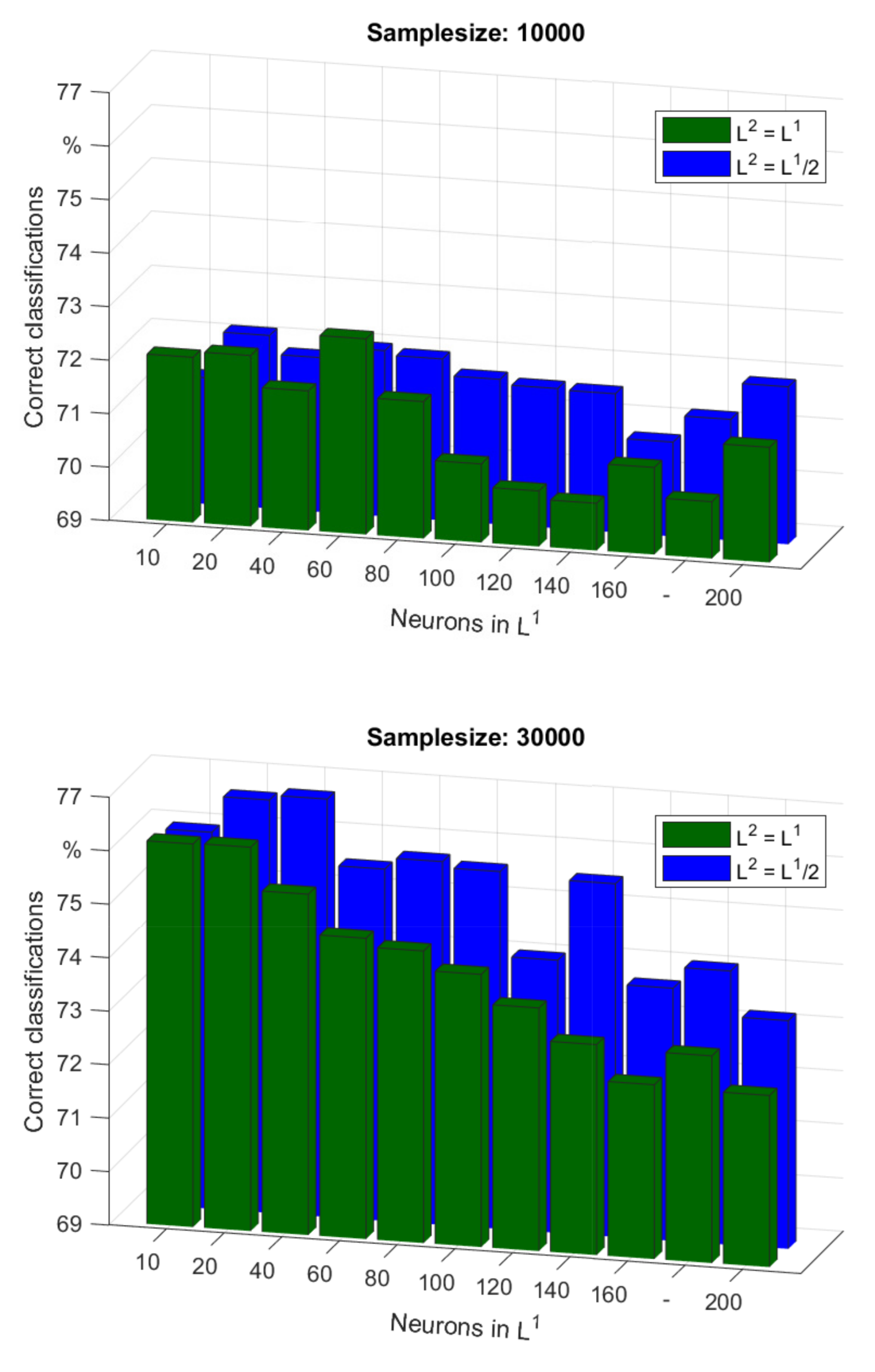
Based on the sample numbers 10,000 and 30,000, the next parameter to be varied is the network size. All previous evaluations and optimizations were based on a four-layer feedforward network with a hidden layer neuron count of 100 and 60, respectively. In the course of the network size optimization, the number of neurons of the hidden layers is now changed. The number of neurons in the first hidden layer L¹ is varied systematically between 10 and 200 neurons. For the number of neurons of the second hidden layer L² the values L² = L¹ and L² = L¹/2 are analyzed, respectively. The obtained success rates can be seen in Figure 8 as a function of network size.

The focus in the following is on a sample number of 30,000, as the maximum success rate could be achieved. Additionally, the corresponding values for a sample number of 10,000 are also listed in brackets, if the application enforces a faster classification.

Table 7. Optimized network architecture with the most important training parameters for a sample number of 30,000 (for a sample number of 10,000 in parentheses).

Parameter	Value/Setting
Neurons—input layer	15,000 (5000)
Neurons—hidden layer 1	40 (60)
Neurons—hidden layer 2	20 (60)
Neurons—output layer	2 (2)
Activation function—hidden layers	tansig
Transfer function—output layer	softmax
Error measure	mean squared error (mse)
Training function	Scaled Conjugate Gradient Backpropagation
Early Stopping	80 epochs
Input signal	normalized FFT

shows the network size and the most important training parameters for the optimized networks. The average success rate can be increased to 77%.

Table 8. Success rates for the optimized network architecture for a sample number of 30,000 and 10,000.

No. of Samples	Success Rate 30 k Samples	Success Rate 10 k Samples
Date 1	64.1%	57.2%
Date 2	89.6%	74.2%
Date 3	61.7%	75.8%
Date 4	91.8%	83.5%
Average	76.8%	72.7%

lists the achieved success rates for the classifications of each measurement date. Compared to the results of the reference network in Table 4 the classification is improved in all dates and for both network sizes. It is surprising that the success rate is decreasing with the number of neurons. Please note that we varied the number of layers with similar results. Increasing the number of layers and therefore the degrees of freedom of the ANN did not improve the success rate. With an average of 77% correct classifications a system can be built to automatically determine the general state of a print head. It is not sufficient to be sure whether a specific nozzle is functional or not, but it is sufficient to estimate if the print head needs maintenance. Therefore, a tool for predictive maintenance of piezo print heads can be built based on our results. An example of the confidence interval for an estimation of functional nozzles will be described in the next section.

4. Industrial Applicability

In the following, a fictitious test case is discussed, in which the complete print head is checked by the final ANN and the number of functioning nozzles is estimated. First of all, the time needed to record the acoustic data is calculated in advance. As already described, this depends directly on the number of samples and can be calculated T_30,000 = 480 s for $n_{sample}$ = 30,000 and T_10,000 = 160 s for $n_{sample}$ = 10,000. The extent to which the reduction in recording time (number of samples) and the associated success rate reduction affect the estimate of the number of functional nozzles can also be subsequently determined by the test case.

For the fictitious test case, it is assumed that the acoustic signals of all 768 nozzles are successively tested by the ANN and that the network evaluates an exemplary 454 nozzles as functional and, accordingly, 314 as clogged. By determining a confidence interval as well as a backward calculation, the number of estimated functional nozzles with a confidence level of 95% is to be determined. The following boundary conditions are known for this purpose.

$$n_{\mathit{functional}}+n_{\mathit{clogged}}=768$$

(5)

$$n_{\mathit{functional}}·T{Q}_{\mathit{functional}}+n_{\mathit{clogged}}·(100-T{Q}_{\mathit{clogged}})=454$$

(6)

As can be seen from the above Equations, the boundary conditions represent a system of two Equations, which has the unknowns n_functional and n_clogged. TQ_functional and TQ_clogged are the success rates for a functional and for a clogged nozzle, respectively. This distinction is necessary because a functional nozzle is detected with a lower probability than a stuck nozzle.

Equations (5) and (6) give an overview of the boundary conditions for determining the estimated functional nozzles n_functional of the print head. First, the sum of estimated functional nozzles n_functional and estimated clogged nozzles n_clogged must be equal to the total number of all nozzles of the print head. On the other hand, the given number of 454 functional nozzles results from the sum of all estimated functional nozzles which were correctly classified as functional nozzles and the number of estimated stuck nozzles which were incorrectly classified as functional by the algorithm. As the two success rates are subject to certain uncertainties, they are to be described as confidence intervals, which corresponds to an estimate of the mean with a given confidence level. Due to the fact that the nozzle state has exactly two possible characteristics (nozzle functional or nozzle clogged), the present case is a Bernoulli process, which leads to a binomial distribution of the success rates. For this, the respective confidence interval can be determined according to Clopper–Pearson [23]. For a number of 1000 test values and a confidence level of 95%, the calculated confidence interval depending on the number of samples can be taken from

Table 9. Confidence intervals for the success rates depending on the number of utilized samples in the signal.

	Confidence Interval 95%	Number of Samples
TQfunctional	70.34–75.92%	30,000
100 − TQclogged	16.70–21.68%	30,000
TQfunctional	63.99–69.91%	10,000
100 − TQclogged	21.09–26.46%	10,000

.

By solving the system of Equations given by Equations (5) and (6) with the aid of the mapped intervals for the success rates from Table 9, a range can now be determined in which the number of estimated functional nozzles of the print head is located with a confidence level of 95%. This range is listed for the sample numbers 30,000 and 10,000 in

Table 10. Confidence intervals for an estimation of functional nozzles.

Number of Nozzles	Number of Samples
530–608	30,000
577–681	10,000

.

Table 10 shows that for a sample number of 30,000, the interval for the number of estimated functional nozzles is 530–608. With a probability of 95%, the number of functional nozzles of the print head is in this range. In comparison, the number of estimated functional nozzles for a sample number of 10,000 is in a range of 577–681. The lower overall success rate for a sample number of 10,000 leads to a spreading of the interval and thus to a less accurate estimation of the real number of nozzles.

The decision whether a sample number of 30,000 or 10,000 should be chosen for the recording of the acoustic depends on the specific use case. It must be determined according to the application whether a less accurate estimation is justifiable and thus the recording time can be reduced by a factor of three (calculated with Equation (3)).

5. Conclusions

In this article, a feasibility study was conducted on defect detection on the print head of a binder jetting 3D printing system with an inorganic molding material system using analysis of structure-born noise. As an analytical evaluation of the acoustic signals did not prove to be feasible, an ANN was used for the analysis of the audio data. It was found that the functionality of the nozzle can be determined on the basis of acoustic patterns in the signal. By optimizing the network parameters and a preprocessing step, a maximum success rate of 76.8% could be achieved based on the acceleration measurements of the print head. With this approach an automatic print head monitoring can be implemented, which is accurate enough to determine whether the print head needs maintenance.

References

1. Gibson, I.; Rosen, D.; Stucker, B.; Khorasani, M. (Eds.) Additive Manufacturing Technologies; Springer International Publishing: Cham, Switzerland, 2021. [Google Scholar] [CrossRef]
2. Sivarupan, T.; Balasubramani, N.; Saxena, P.; Nagarajan, D.; El Mansori, M.; Salonitis, K.; Jolly, M.; Dargusch, M.S. A review on the progress and challenges of binder jet 3D printing of sand moulds for advanced casting. Addit. Manuf. 2021, 40, 101889. [Google Scholar] [CrossRef]
3. Ramakrishnan, R.; Griebel, B.; Volk, W.; Günther, D.; Günther, J. 3D Printing of Inorganic Sand Moulds for Casting Applications. Adv. Mater. Res. 2014, 1018, 441–449. [Google Scholar] [CrossRef]
4. Liu, H.; Lei, T.; Ma, C.; Peng, F. Optimization of driven waveform of piezoelectric printhead for 3D sand-printing. Addit. Manuf. 2021, 37, 101627. [Google Scholar] [CrossRef]
5. Lechner, P.; Hartmann, C.; Ettemeyer, F.; Volk, W. A Plane Stress Failure Criterion for Inorganically-Bound Core Materials. Materials 2021, 14, 247. [Google Scholar] [CrossRef] [PubMed]
6. Pabel, T.; Kneißl, C.; Brotzki, J.; Müller, J. Anorganisches Bindersystem. GIESSEREI-PRAXIS, 1 November 2009. [Google Scholar]
7. Mostafaei, A.; Elliott, A.M.; Barnes, J.E.; Li, F.; Tan, W.; Cramer, C.L.; Nandwana, P.; Chmielus, M. Binder jet 3D printing—Process parameters, materials, properties, modeling, and challenges. Prog. Mater. Sci. 2021, 119, 100707. [Google Scholar] [CrossRef]
8. Polzin, H. Inorganic Binders: For Mould and Core Production in the Foundry; Fachverlag Schiele & Schön: Berlin, Germany, 2014. [Google Scholar]
9. Gunther, D.; Pirehgalin, M.F.; Weis, I.; Vogel-Heuser, B. Condition monitoring for the Binder Jetting AM-process with machine learning approaches. In Proceedings of the 2020 IEEE Conference on Industrial Cyberphysical Systems (ICPS), Tampere, Finland, 10–12 June 2020; pp. 417–420. [Google Scholar] [CrossRef]
10. Lechner, P.; Fuchs, G.; Hartmann, C.; Steinlehner, F.; Ettemeyer, F.; Volk, W. Acoustical and Optical Determination of Mechanical Properties of Inorganically-Bound Foundry Core Materials. Materials 2020, 13, 2531. [Google Scholar] [CrossRef] [PubMed]
11. Swarnakar, A.K.; van der Biest, O.; Vanhellemont, J. Determination of the Si Young’s modulus between room and melt temperature using the impulse excitation technique. Phys. Status Solidi C 2014, 11, 150–155. [Google Scholar] [CrossRef]
12. Dornfeld, D. Application of acoustic emission techniques in manufacturing. NDT & E Int. 1992, 25, 259–269. [Google Scholar] [CrossRef]
13. Shevchik, S.A.; Kenel, C.; Leinenbach, C.; Wasmer, K. Acoustic emission for in situ quality monitoring in additive manufacturing using spectral convolutional neural networks. Addit. Manuf. 2018, 21, 598–604. [Google Scholar] [CrossRef]
14. der Mauer, M.A.; Behrens, T.; Derakhshanmanesh, M.; Hansen, C.; Muderack, S. Applying Sound-Based Analysis at Porsche Production: Towards Predictive Maintenance of Production Machines Using Deep Learning and Internet-of-Things Technology. In Digitalization Cases; Management for Professionals; Urbach, N., Röglinger, M., Eds.; Springer International Publishing: Cham, Switzerland, 2019; Volume 29, pp. 79–97. [Google Scholar] [CrossRef]
15. Ramakrishnan, R. 3-D-Drucken Mit Einem Anorganischen Formstoffsystem. Ph.D. Thesis, Institut für Umformtechnik und Gießereiwesen (utg), Technische Universität München, München, Germany, 2015. [Google Scholar]
16. Kistler. Produktdatenblatt K-Shear Beschleunigungssensoren: Universale Beschleunigunssensoren mit Spannungsausgang; Kistler Instrumente AG: Munich, Germany, 2008. [Google Scholar]
17. Kistler. Produktdatenblatt Montagezubehör für Beschleunigungssensoren; Kistler Instrumente AG: Munich, Germany, 2006. [Google Scholar]
18. MathWorks. Classify Patterns with a Shallow Neural Network. Available online: https://de.mathworks.com/help/nnet/gs/classify-patterns-with-a-neural-network.html (accessed on 22 August 2021).
19. MathWorks. Choose a Multilayer NN Training Function. Available online: https://de.mathworks.com/help/nnet/ug/choose-a-multilayer-neural-network-training-function.html (accessed on 22 August 2021).
20. Hagan, M.T.; Demuth, H.B.; Beale, M.; De Jesus, O. Neural Network Design, 2nd ed.; Martin Hagan: Frisco, TX, USA, 2014. [Google Scholar]
21. Schaffer, C. Selecting a classification method by cross-validation. Mach. Learn. 1993, 13, 135–143. [Google Scholar] [CrossRef]
22. Runkler, T.A. Data Mining: Modelle und Algorithmen Intelligenter Datenanalyse, 2. Aktualisierte Aufl. ed.; Computational Intelligence; Springer Fachmedien Wiesbaden: Wiesbaden, Germany, 2015. [Google Scholar]
23. Clopper, C.J.; Pearson, E.S. The Use of Confidence or Fiducial Limits Illustrated in the Case of the Binomial. Biometrika 1934, 26, 404–413. [Google Scholar] [CrossRef]
Figure 1. Mounting of the acceleration sensor on the print head. Highlighted are the accelerometer (1), the threaded nut for position assurance (2), the threaded nut for clamping (3), the spacer plate (4), and the surrounding steel plate (5).
Applsci 11 10672 g001
Figure 2. Flow chart for the recording of 30 nozzle shots in one data block.
Applsci 11 10672 g002
Figure 3. Comparison of the signal amplitudes of the individual data blocks in the time domain.
Applsci 11 10672 g003
Figure 4. Spectral analysis for a shot with a functional and a clogged nozzle.
Applsci 11 10672 g004
Figure 5. Confusion matrix measuring date 3 evaluated with the reference network.
Applsci 11 10672 g005
Figure 6. Confusion matrices for measurement dates 1 and 3 after the signal was normalized in the time domain in a preprocessing step.
Applsci 11 10672 g006
Figure 7. The success rate of the classification depends on the number of samples in the recording and therefore the recording length.
Applsci 11 10672 g007
Figure 8. Success rates for different sizes of the hidden layers in the ANN.
Applsci 11 10672 g008