State-Feedback Control in Descriptor Discrete-Time Fractional-Order Linear Systems: A Superstability-Based Approach

Abstract

In this article, the superstabilizing state-feedback control problem in descriptor discrete-time fractional-order linear (DDFL) systems with a regular matrix pencil is studied. Methods for investigating the stability and superstability of the considered class of dynamical systems are presented. Procedures for the computation of the static state-feedback (SSF) and dynamic state-feedback (DSF) gain matrices such that the closed-loop DDFL (CL-DDFL) system is superstable are presented. A numerical example is used to show the efficacy of the presented approach. Our considerations were based on the Drazin inverse matrix method.

1. Introduction

Descriptor systems (also known as singular systems) play an important role in modern control theory, allowing us to model and analyze constrained dynamical systems [1,2,3]. These restrictions can be naturally imposed on a system (as a consequence of physical laws, e.g., the law of conservation of energy) or determined by the engineer (e.g., the constrained area of work).

In the second half of the 20th century, many papers and monographs on descriptor systems were written, laying the foundations for this theory [4,5,6,7,8,9,10,11]. An overview of the state of the art in the field of descriptor systems theory can be found in [1,2,3,7]. The stability of such systems was examined in [2,3,7,12,13]. Static and dynamic feedback control in descriptor systems was also investigated for state feedback [2,7,14] and the output feedback [2,7,15,16,17]. Descriptor systems theory can be used in many areas, such as electrical and mechanical engineering, robotics, fluid mechanics, chemical engineering, economics, and demography, see e.g., [2,4,8,18,19,20].

In recent years, the analysis and synthesis problems of dynamical systems described by fractional-order differential (or difference) equations have attracted a lot of attention [3,20,21,22,23].

The notion of the practical stability of positive fractional discrete-time systems was introduced in [24] and conditions for practical stability were provided in [24,25]. The stability of discrete-time linear systems with delays was investigated in [26,27].

Superstable systems are a subclass of asymptotically stable systems, in which dynamics are more restricted. Such systems provide some practically important properties, e.g., superstability (as opposed to stability) remains under the presence of time-varying and nonlinear perturbations, which allows researchers to solve problems relating to the synthesis of robust systems easily. Moreover, superstable systems ensure the elimination of peaks or sharp increases in the state vector trajectory [28,29,30].

In this article, the superstabilizing state-feedback control problem in DDFL systems is studied. The main advantage of the presented approach is that it can be applied to the analysis of descriptor systems properties which are determined by matrix entries, such as positivity and superstability. This study is an extension of the results presented in [31].

The organization of the paper is as follows. In Section 2 the considered state-space model is introduced. Section 3 is devoted to the application of the Drazin inverse to the analysis of DDFL systems. In Section 4 an equivalent model of this class of dynamical systems is presented. Methods for investigating stability and superstability are given in Section 5. In Section 6 and Section 7 descriptor systems with static and dynamic state-feedback are studied and procedures for the computation of the gain matrices such that the closed-loop system is superstable are given. A numerical example showing the efficacy of the discussed approach is presented in Section 8. In Section 9 some concluding remarks and open problems are provided.

The following system of symbols will be used in the paper: $\mathbb{R}$ for the set of real numbers, ${\mathbb{R}}^{n\times m}$ for the set of $n\times m$ real matrices, $\mathbb{C}$ for the set of complex numbers, ${\mathbb{Z}}_{+}$ for the set of nonnegative integers, and ${\mathbb{I}}_n$ for the $n\times n$ identity matrix.

2. Considered State-Space Model

Let us consider the DDFL system in the form

$$E{\mathsf{\Delta }}^{\alpha }{x}_{i+1}=A{x}_i+B{u}_i,0<\alpha <1,i\in {\mathbb{Z}}_{+},$$

(1)

where $x_i\in {\mathbb{R}}^n$ is the state vector, $u_i\in {\mathbb{R}}^m$ is the input vector, $E,A\in {\mathbb{R}}^{n\times n}$, $B\in {\mathbb{R}}^{n\times m}$ and ${\mathsf{\Delta }}^{\alpha }{x}_i$ is the Grünwald–Letnikov fractional-order backward difference defined by [21]

$${\mathsf{\Delta }}^{\alpha }{x}_i=\sum _{j=0}^i{(-1)}^j\left(\genfrac{}{}{0pt}{}{\alpha }{j}\right)x_{i-j},$$

(2)

where

$$\left(\genfrac{}{}{0pt}{}{\alpha }{j}\right)=\left\{\begin{array}{cc}1\hfill & \mathrm{for}j=0,\hfill \\ \frac{\alpha (\alpha -1)\dots (\alpha -j+1)}{j!}\hfill & \mathrm{for}j=1,2,3,\dots .\hfill \end{array}\right.$$

(3)

In descriptor systems $\det E=0$ and therefore the matrix E is not invertible.

Definition 1.

Let A, B be some matrices of the same size. A set of such matrices of the form $A+\lambda B$ is called a matrix pencil, where λ is a parameter. If A, B are square matrices and $\det [A+\lambda B]\ne 0$, then the pencil is called a regular one.

According to Definition 1 we distinguish two subclasses of descriptor systems:

(1)

with the regular matrix pencil of the pair $(E,A)$, i.e., $\det [E\lambda -A]\ne 0$ for some $\lambda \in \mathbb{C}$;

(2)

with the singular matrix pencil of the pair $(E,A)$, i.e., $\det [E\lambda -A]=0$ for some $\lambda \in \mathbb{C}$.

If the matrix pencil of the pair $(E,A)$ is regular, then the solution of the state equation of a descriptor system exists and it is unique for any consistent initial condition [2,7].

There are several methods for analyzing the system (1) with the regular matrix pencil, which are based on the Drazin inverse [5], the Laurent series expansion [9] and the Weierstrass–Kronecker decomposition [11] methods.

3. Application of the Drazin Inverse

Let us assume that the matrix pencil of the pair $(E,A)$ of the system (1) is regular. As a consequence, we have $\det [Ec-A]\ne 0$ for some $c\in \mathbb{C}$. Premultiplication of (1) by ${[Ec-A]}^{-1}$ yields

$$\overline{E}{\mathsf{\Delta }}^{\alpha }{x}_{i+1}=\overline{A}{x}_i+\overline{B}{u}_i,$$

(4)

where

$$\overline{E}={[Ec-A]}^{-1}E,\overline{A}={[Ec-A]}^{-1}A,\overline{B}={[Ec-A]}^{-1}B.$$

(5)

It is well known that premultiplication of a matrix equation by the nonsingular matrix does not change its solution. Therefore, both Equations (1) and (4) have the same solution $x_i$. The substitution of (2) into (4) yields

$$\overline{E}{x}_{i+1}={\overline{A}}_{\alpha }{x}_i+\sum _{j=1}^i\overline{E}{c}_j{x}_{i-j}+\overline{B}{u}_i,i\in {\mathbb{Z}}_{+},$$

(6)

where

$${\overline{A}}_{\alpha }=\overline{A}+\overline{E}\alpha .$$

(7)

and

$$c_j={(-1)}^j\left(\genfrac{}{}{0pt}{}{\alpha }{j+1}\right).$$

(8)

Observe that the values of the coefficients $c_j$ determined by (8) highly decrease for increasing j. Therefore, in many cases the upper bound of the summation can be limited by some natural number L, which is called the length of practical implementation [24]. Hence, we can write Equation (6) in the form

$$\overline{E}{x}_{i+1}={\overline{A}}_{\alpha }{x}_i+\sum _{j=1}^L\overline{E}{c}_j{x}_{i-j}+\overline{B}{u}_i$$

(9)

with $x_{-k}=0$, $k=1,2,\dots$.

Definition 2

([3,7]). The Drazin inverse of $\overline{E}\in {\mathbb{R}}^{n\times n}$, denoted by ${\overline{E}}^D\in {\mathbb{R}}^{n\times n}$, is a matrix satisfying the following conditions

$$\overline{E}{\overline{E}}^D={\overline{E}}^D\overline{E},{\overline{E}}^D\overline{E}{\overline{E}}^D={\overline{E}}^D,{\overline{E}}^D{\overline{E}}^{q+1}={\overline{E}}^q,$$

(10)

where q is the index of $\overline{E}$, i.e., the smallest nonnegative integer such that

$$\mathrm{rank}{\overline{E}}^q=\mathrm{rank}{\overline{E}}^{q+1}.$$

(11)

Every square matrix has its own unique Drazin inverse [3,5,7]. For a nonsingular matrix the Drazin inverse is equivalent to the standard matrix inverse. Some methods for the computation of the Drazin inverse can be found in [3].

Lemma 1

([3,7]). The properties of the matrices $\overline{E}$ and $\overline{A}$ given by (5) are as follows:

$$\overline{A}\overline{E}=\overline{E}\overline{A},{\overline{E}}^D\overline{A}=\overline{A}{\overline{E}}^D,{\overline{A}}^D\overline{E}=\overline{E}{\overline{A}}^D,{\overline{A}}^D{\overline{E}}^D={\overline{E}}^D{\overline{A}}^D,$$

(12)

$$\ker \overline{A}\cap \ker \overline{E}=\left\{0\right\},$$

(13)

$$({\mathbb{I}}_n-\overline{E}{\overline{E}}^D)\overline{A}{\overline{A}}^D={\mathbb{I}}_n-\overline{E}{\overline{E}}^D,({\mathbb{I}}_n-\overline{E}{\overline{E}}^D){\left(\overline{E}{\overline{A}}^D\right)}^q=0.$$

(14)

$$\overline{E}=T\left[\begin{array}{cc}J& 0\\ 0& N\end{array}\right]T^{-1},{\overline{E}}^D=T\left[\begin{array}{cc}{J}^{-1}& 0\\ 0& 0\end{array}\right]T^{-1},\overline{A}=T\left[\begin{array}{cc}{A}_1& 0\\ 0& A_2\end{array}\right]T^{-1},$$

(15)

where $T\in {\mathbb{R}}^{n\times n}$ and $J\in {\mathbb{R}}^{n_1\times n_1}$ are nonsingular matrices, $N\in {\mathbb{R}}^{n_2\times n_2}$ is a nilpotent matrix, i.e., for some μ we have $N^{\mu -1}\ne 0$, $N^{\mu }=0$ and $A_1\in {\mathbb{R}}^{n_1\times n_1}$, $A_2\in {\mathbb{R}}^{n_2\times n_2}$, $n_1+n_2=n$.

Let $\mathbb{U}\subset {\mathbb{R}}^m$ be the set of admissible inputs $u_i\in \mathbb{U}$ and ${\mathbb{X}}_0\subset {\mathbb{R}}^n$ be the set of consistent initial conditions $x_0\in {\mathbb{X}}_0$ for which Equation (1) has a solution $x_i$ for $u_i\in \mathbb{U}$.

Theorem 1

([3]). The solution to Equation (6) (or equivalently (1)) for $x_0\in {\mathbb{X}}_0$ and $u_i\in \mathbb{U}$ is given by

$$x_i={\mathsf{\Phi }}_i^{\left({\overline{E}}^D{\overline{A}}_{\alpha }\right)}\overline{E}{\overline{E}}^{D}v+\sum _{k=0}^{i-1}{\mathsf{\Phi }}_{i-k-1}^{\left({\overline{E}}^D{\overline{A}}_{\alpha }\right)}{\overline{E}}^D\overline{B}{u}_k+(\overline{E}{\overline{E}}^D-{\mathbb{I}}_n)\sum _{k=0}^{q-1}{\left(\overline{E}{\overline{A}}^D\right)}^k{\overline{A}}^D\overline{B}{\psi }_{i,k},$$

(16)

where the vector $v\in {\mathbb{R}}^n$ is arbitrary, q is the index of $\overline{E}$ determined by (11) and

$${\mathsf{\Phi }}_{i+1}^{\left({\overline{E}}^D{\overline{A}}_{\alpha }\right)}={\mathsf{\Phi }}_i^{\left({\overline{E}}^D{\overline{A}}_{\alpha }\right)}{\overline{E}}^D{\overline{A}}_{\alpha }+\sum _{j=1}^i{c}_j{\mathsf{\Phi }}_{i-j}^{\left({\overline{E}}^D{\overline{A}}_{\alpha }\right)},{\mathsf{\Phi }}_0^{\left({\overline{E}}^D{\overline{A}}_{\alpha }\right)}={\mathbb{I}}_n,$$

(17)

$$\begin{array}{cc}\hfill {\psi }_{i,0}=& u_i,\hfill \\ \hfill {\psi }_{i,1}=& {\psi }_{i+1,0}-\alpha {\psi }_{i,0}-\sum _{j=1}^i{c}_j{\psi }_{i-j,0}\hfill \\ \hfill =& u_{i+1}-\alpha u_i-\sum _{j=1}^i{c}_j{u}_{i-j},\hfill \\ \hfill {\psi }_{i,2}=& {\psi }_{i+1,1}-\alpha {\psi }_{i,1}-\sum _{j=1}^i{c}_j{\psi }_{i-j,1}\hfill \\ \hfill =& u_{i+2}-2\alpha u_{i+1}+{\alpha }^2{u}_i+2\alpha \sum _{j=1}^i{c}_j{u}_{i-j}-\sum _{j=1}^{i+1}{c}_j{u}_{i-j+1}\hfill \\ & -\sum _{j=1}^i{c}_j{u}_{i-j+1}+\sum _{j=1}^i{c}_j\sum _{l=1}^{i-j}{c}_l{u}_{i-j-l}\hfill \\ \hfill ⋮& \\ \hfill {\psi }_{i,q-1}& ={\psi }_{i+1,q-2}-\alpha {\psi }_{i,q-2}-\sum _{j=1}^i{c}_j{\psi }_{i-j,q-2}.\hfill \end{array}$$

(18)

For any admissible $u_i\in \mathbb{U}$ the consistent initial conditions should satisfy the equality

$$x_0=\overline{E}{\overline{E}}^{D}v+(\overline{E}{\overline{E}}^D-{\mathbb{I}}_n)\sum _{k=0}^{q-1}{\left(\overline{E}{\overline{A}}^D\right)}^k{\overline{A}}^D\overline{B}{\psi }_{0,k},$$

(19)

which is obtained from (16) and (17) for $i=0$, the vector $v\in {\mathbb{R}}^n$ is arbitrary and ${\psi }_{0,k}\in {\mathbb{R}}^m$ is given by (18). The solution (16) of (1) for $x_0\in {\mathbb{X}}_0$ can be computed, substituting $v=x_0$.

Observe that the matrices (5) and their Drazin inverses appear in the solution (16) as products $\overline{E}{\overline{E}}^D$, ${\overline{E}}^D\overline{A}$, ${\overline{A}}^D\overline{E}$, ${\overline{E}}^D\overline{B}$, ${\overline{A}}^D\overline{B}$. This is an important property since these products do not depend on the choice of the parameter c, unlike the matrices $\overline{E}$, $\overline{A}$, $\overline{B}$ themselves [7].

4. Equivalent State-Space Model

We shall show that Equation (4) is equivalent to two equations (subsystems). Based on [3,31] we obtain the following. To simplify the notation we introduce

$${\overline{A}}_1={\overline{E}}^D\overline{A},{\overline{B}}_1={\overline{E}}^D\overline{B},{\overline{B}}_2=({\mathbb{I}}_n-\overline{E}{\overline{E}}^D){\overline{A}}^D\overline{B},\overline{N}=({\mathbb{I}}_n-\overline{E}{\overline{E}}^D){\overline{A}}^D\overline{E}.$$

(20)

Lemma 2

([3]). Let

$$x_{1,i}=\overline{E}{\overline{E}}^D{x}_i,x_{2,i}=({\mathbb{I}}_n-\overline{E}{\overline{E}}^D)x_i,$$

(21)

$$x_{1,i}+x_{2,i}=x_i.$$

(22)

Equation (4) can be decomposed into the following equations:

$${\mathsf{\Delta }}^{\alpha }{x}_{1,i+1}={\overline{A}}_1{x}_{1,i}+{\overline{B}}_1{u}_i,$$

(23)

$$\overline{N}{\mathsf{\Delta }}^{\alpha }{x}_{2,i+1}=x_{2,i}+{\overline{B}}_2{u}_i.$$

(24)

Substituting (2) into (23)–(24) and introducing the length L of practical implementation (the constraint on the upper limit of the summation), as in the case of (9), gives

$$x_{1,i+1}={\overline{A}}_{1\alpha }{x}_{1,i}+\sum _{j=1}^L{c}_j\overline{E}{\overline{E}}^D{x}_{1,i-j}+{\overline{B}}_1{u}_i,$$

(25)

$$\overline{N}{x}_{2,i+1}=({\mathbb{I}}_n+\overline{N}\alpha )x_{2,i}+\sum _{j=1}^L{c}_j\overline{N}{x}_{2,i-j}+{\overline{B}}_2{u}_i,$$

(26)

where $\overline{N}$ is a nilpotent matrix with the nilpotency index q and

$${\overline{A}}_{1\alpha }={\overline{A}}_1+\overline{E}{\overline{E}}^D\alpha .$$

(27)

It is not difficult to verify that the solution (16) is the sum of solutions to Equations (25) and (26) for $L=i$.

5. Stability and Superstability Analysis

Methods for investigating the stability and superstability of DDFL systems will be presented in this section.

5.1. Stability Analysis

Definition 3.

The DDFL system (1) with $u_i=0$, $i\in {\mathbb{Z}}_{+}$ is called asymptotically stable if

$$\underset{i\to \infty }{lim}{x}_i=0$$

(28)

for all consistent initial conditions $x_0\in {\mathbb{X}}_0$.

From the solution to Equation (26), which is a third component of (16), it follows that for $u_i=0$ the vector $x_{2,i}$ is equal to zero for any $i\in {\mathbb{Z}}_{+}$. Taking into account (22), the stability of the DDFL system (1) depends only on the vector $x_{1,i}$, which is a solution to Equation (25).

The stability of the DDFL system (1) can be tested using well-known methods in the literature; see, e.g., [27]. For the analysis, either Equation (6) or (25) can be used.

Definition 4.

The DDFL system (1) is called practically stable for given length L of practical implementation if the DDFL system (9) (or equivalently (25)) is asymptotically stable. If the DDFL system (9) (or equivalently (25)) is asymptotically stable for $L\to \infty$, then the DDFL system (1) is called asymptotically stable (independent of L).

Theorem 2

([3]). The DDFL system (1) with given length L of practical implementation is practically stable if and only if all roots of the characteristic equation

$$\det \left[\overline{E}z-{\overline{A}}_{\alpha }-\sum _{j=1}^L\overline{E}{c}_j{z}^{-j}\right]=0$$

(29)

are located inside the unit circle.

Taking into account that [32]

$$\sum _{j=1}^{\infty }{c}_j{z}^{-j}=z-\alpha -{(z-1)}^{\alpha }{z}^{1-\alpha }$$

(30)

from (29) we obtain the following.

Theorem 3

([3]). The DDFL system (1) is asymptotically stable (independent of L) if and only if all roots of the characteristic equation

$$\det \left[\overline{E}{(z-1)}^{\alpha }{z}^{1-\alpha }-\overline{A}\right]=0$$

(31)

are located inside the unit circle.

The stability of the DDFL system (1) can also be tested using the approach based on the Equation (25).

Lemma 3.

The characteristic equation of (25) has the form

$$\det \left[{\mathbb{I}}_{n}z-{\overline{A}}_{1\alpha }-\sum _{j=1}^L\overline{E}{\overline{E}}^D{c}_j{z}^{-j}\right]=z^{n-r}\det \left[\overline{E}z-{\overline{A}}_{\alpha }-\sum _{j=1}^L\overline{E}{c}_j{z}^{-j}\right]=0$$

(32)

and it has $r=\mathrm{rank}{\overline{A}}_1$ roots of the characteristic Equation (29) along with additional $n-r$ zero-valued eigenvalues.

Proof. 

Using (15) we have

$$\begin{array}{cc}\hfill \det \left[\overline{E}z-{\overline{A}}_{\alpha }-\sum _{j=1}^L\overline{E}{c}_j{z}^{-j}\right]& =\det \left\{T\left[\begin{array}{cc}J\lambda -A_1& 0\\ 0& N\lambda -A_2\end{array}\right]T^{-1}\right\}\hfill \\ & =\det T\det [J\lambda -A_1]\det [N\lambda -A_2]\det T^{-1}\hfill \\ & =\det [J\lambda -A_1]\det [N\lambda -A_2]\hfill \end{array}$$

(33)

since $\det T\det T^{-1}={\mathbb{I}}_n$ and

$$\lambda =\left(z-\alpha -\sum _{j=1}^L{c}_j{z}^{-j}\right).$$

(34)

Again using (15), we can write

$$\begin{array}{cc}\hfill \det \left[{\mathbb{I}}_{n}z-{\overline{A}}_{1\alpha }-\sum _{j=1}^L\overline{E}{\overline{E}}^D{c}_j{z}^{-j}\right]& =\det \left\{T\left[\begin{array}{cc}{\mathbb{I}}_{n_1}\lambda -J^{-1}{A}_1& 0\\ 0& {\mathbb{I}}_{n_2}z\end{array}\right]T^{-1}\right\}\hfill \\ & =\det T\det [{\mathbb{I}}_{n_1}\lambda -J^{-1}{A}_1]\det \left[{\mathbb{I}}_{n_2}z\right]\det T^{-1}\hfill \\ & =z^{n_2}\det [{\mathbb{I}}_{n_1}\lambda -J^{-1}{A}_1]\hfill \end{array}$$

(35)

since $\det T\det T^{-1}={\mathbb{I}}_n$ and $\lambda$ is given by (34). By (12) we have $\overline{E}\overline{A}=\overline{A}\overline{E}$ and from (15) it follows that $N{A}_2=A_{2}N$ if and only if $A_2=\gamma {\mathbb{I}}_{n_2}$, where $\gamma \in \mathbb{R}$, i.e., $A_2$ is a scalar matrix. Therefore, Equation (33) can be written as

$$\begin{array}{cc}\hfill \det [J\lambda -A_1]\det [N\lambda -\gamma {\mathbb{I}}_{n_2}]& ={(-\gamma )}^{n_2}\det [J\lambda -A_1]\hfill \\ & ={(-\gamma )}^{n_2}\det [{\mathbb{I}}_{n_1}\lambda -J^{-1}{A}_1]\hfill \end{array}$$

(36)

since $\det [N\lambda -\gamma {\mathbb{I}}_{n_2}]={(-\gamma )}^{n_2}$. Equating (33) and (36) to zero and denoting $n_1=r$ and $n_2=n-r$ we obtain (32). □

Taking into account the above considerations, the following theorems can be formulated.

Theorem 4.

The DDFL system (1) is practically stable for a given length L of practical implementation if and only if $r=\mathrm{rank}{\overline{A}}_1$ roots of the characteristic equation

$$\begin{array}{c}\hfill \det \left[{\mathbb{I}}_{n}z-{\overline{A}}_{1\alpha }-\sum _{j=1}^L\overline{E}{\overline{E}}^D{c}_j{z}^{-j}\right]=0\end{array}$$

(37)

lie inside the unit circle and $n-r$ its remaining roots are zero-valued.

Theorem 5.

The DDFL system (1) is asymptotically stable (independent of L) if and only if $r=\mathrm{rank}{\overline{A}}_1$ roots of the characteristic equation

$$\begin{array}{c}\hfill \det \left[({\mathbb{I}}_n-\overline{E}{\overline{E}}^D)z-{\overline{A}}_1+\overline{E}{\overline{E}}^D{(z-1)}^{\alpha }{z}^{1-\alpha }\right]=0\end{array}$$

(38)

lie inside the unit circle and $n-r$ its remaining roots are zero-valued.

5.2. Superstability Analysis

The value of the free response of an asymptotically stable system decreases to zero over time, but it may considerably increase in the initial part of the trajectory. In superstable systems, which are a subclass of asymptotically stable systems, state variables are limited by the value of the norm of the state vector, which decreases monotonically to zero over time [28,29,30].

Furthermore, the problems of static output stabilization, the simultaneous stabilization of more than one system, robust stabilization under matrix uncertainty, etc., are solved easily for superstable systems [29].

In this paper the following vector and matrix norms will be used:

• the infinity-norm of a vector $x_i=\left[x_{i,k}\right]\in {\mathbb{R}}^n$

  $$\parallel x_i\parallel =\underset{1\le k\le n}{max}\left|x_{i,k}\right|,$$

  (39)
• the infinity-norm of a matrix $A=\left[a_{ij}\right]\in {\mathbb{R}}^{n\times n}$

  $$\parallel A\parallel =\underset{1\le i\le n}{max}\left(\sum _{j=1}^n\left|a_{ij}\right|\right).$$

  (40)

Definition 5

([29]). A matrix $A=\left[a_{ij}\right]\in {\mathbb{R}}^{n\times n}$ of the discrete-time linear system

$$x_{i+1}=A{x}_i$$

(41)

is called superstable if

$$\sigma \left(A\right)=\sigma =1-\parallel A\parallel >0$$

(42)

or equivalently

$$\parallel A\parallel <1,$$

(43)

where the quantity σ is called the superstability degree of the matrix A.

A superstable matrix is also a stable one, but the reverse implication is not true (a stable matrix may not be a superstable one).

Theorem 6

([29]). For the superstable discrete-time linear system (41) the following holds:

$$\parallel x_i\parallel \le {\sigma }^i\parallel x_0\parallel ,i\in {\mathbb{Z}}_{+}.$$

(44)

Now let us consider the DDFL system (1). From (25) and (26) for $u_i=0$, $i\in {\mathbb{Z}}_{+}$ we have

$$x_i=x_{1,i}=\overline{E}{\overline{E}}^D{x}_i,i\in {\mathbb{Z}}_{+}$$

(45)

since $x_{2,i}=0$. Taking into account (45) and $({\mathbb{I}}_n-\overline{E}{\overline{E}}^D)\overline{E}{\overline{E}}^D=0$, Equation (25) for $u_i=0$, $i\in {\mathbb{Z}}_{+}$ can also be written as

$$x_{i+1}=\overline{F}{x}_i+\sum _{j=1}^L{c}_j\overline{E}{\overline{E}}^D{x}_{i-j},$$

(46)

where

$$\overline{F}={\overline{A}}_{1\alpha }+\overline{G}({\mathbb{I}}_n-\overline{E}{\overline{E}}^D)$$

(47)

and the matrix $\overline{G}\in {\mathbb{R}}^{n\times n}$ is arbitrary.

In descriptor systems the matrix ${\overline{A}}_{1\alpha }$ acts as a pseudo-state matrix. From the solution of Equation (23) it follows that ${\overline{A}}_{1\alpha }$ may contain insignificant entries that are further reduced through multiplication by $x_0\in \mathrm{Im}\overline{E}{\overline{E}}^D$. To eliminate such entries from the matrix ${\overline{A}}_{1\alpha }$ we can use the term $\overline{G}({\mathbb{I}}_n-\overline{E}{\overline{E}}^D)$, which does not change the solution to the state equation [3,31].

Taking into consideration (16) and (45) the solution to Equation (46) for $v=x_0$ can be expressed by

$$x_i={\mathsf{\Phi }}_i^{\left(\overline{F}\right)}\overline{E}{\overline{E}}^D{x}_0,$$

(48)

where

$${\mathsf{\Phi }}_{i+1}^{\left(\overline{F}\right)}={\mathsf{\Phi }}_i^{\left(\overline{F}\right)}\overline{F}+\sum _{j=1}^L{c}_j{\mathsf{\Phi }}_{i-j}^{\left(\overline{F}\right)},{\mathsf{\Phi }}_0^{\left(\overline{F}\right)}={\mathbb{I}}_n,{\mathsf{\Phi }}_{-k}^{\left(\overline{F}\right)}=0,k=1,2,\dots .$$

(49)

Let us introduce the definition of practical superstability for DDFL systems, analogous to the definition of practical stability given in Section 5.1.

Definition 6.

The DDFL system (1) is called practically superstable for a given length L of practical implementation if the DDFL system (46) is superstable. If the DDFL system (46) is superstable for $L\to \infty$, then the DDFL system (1) is called superstable (independent of L).

Theorem 7.

The DDFL system (46) is superstable if there exists an arbitrary matrix $\overline{G}\in {\mathbb{R}}^{n\times n}$ such that

$$\parallel \overline{F}\parallel \in \left(\frac{d-\sqrt{d^2-4c_L}}{2};\frac{d+\sqrt{d^2-4c_L}}{2}\right)\mathrm{for}L\ge 1$$

(50)

or

$$\parallel \overline{F}\parallel <1\mathrm{for}L=0,$$

(51)

where the matrix $\overline{F}$ is defined by (47) and

$$d=1-\sum _{j=1}^{L-1}{c}_j.$$

(52)

Proof. 

From Theorem 6 it follows that for a superstable system we have $\parallel x_{i+1}\parallel <\parallel x_i\parallel$. Let us assume that the DDFL system (46) is superstable. Hence, we obtain

$$\frac{∥{\mathsf{\Phi }}_{i+1}^{\left(\overline{F}\right)}∥}{∥{\mathsf{\Phi }}_i^{\left(\overline{F}\right)}∥}<1,i\in {\mathbb{Z}}_{+}$$

(53)

since $\parallel x_i\parallel \le ∥{\mathsf{\Phi }}_i^{\left(\overline{F}\right)}∥∥\overline{E}{\overline{E}}^D{x}_0∥$. Taking into account that

$$∥{\mathsf{\Phi }}_{i+1}^{\left(\overline{F}\right)}∥\le ∥{\mathsf{\Phi }}_i^{\left(\overline{F}\right)}∥\parallel \overline{F}\parallel +∥\sum _{j=1}^L{c}_j{\mathsf{\Phi }}_{i-j}^{\left(\overline{F}\right)}∥$$

(54)

the inequality (53) can be rewritten as [3]

$$\begin{array}{cc}\hfill \frac{∥{\mathsf{\Phi }}_{i+1}^{\left(\overline{F}\right)}∥}{∥{\mathsf{\Phi }}_i^{\left(\overline{F}\right)}∥}& \le \parallel \overline{F}\parallel +\frac{∥{\displaystyle \sum _{j=1}^L}{c}_j{\mathsf{\Phi }}_{i-j}^{\left(\overline{F}\right)}∥}{∥{\mathsf{\Phi }}_i^{\left(\overline{F}\right)}∥}\hfill \\ & \le \parallel \overline{F}\parallel +\frac{∥\left[\begin{array}{cccc}{c}_1{\mathbb{I}}_n& c_2{\mathbb{I}}_n& \dots & c_L{\mathbb{I}}_n\end{array}\right]\left[\begin{array}{c}{\mathsf{\Phi }}_{i-1}^{\left(\overline{F}\right)}\\ {\mathsf{\Phi }}_{i-2}^{\left(\overline{F}\right)}\\ ⋮\\ {\mathsf{\Phi }}_{i-L}^{\left(\overline{F}\right)}\end{array}\right]∥}{∥\left[\begin{array}{cccc}\overline{F}& c_1{\mathbb{I}}_n& \dots & c_{L-1}{\mathbb{I}}_n\end{array}\right]\left[\begin{array}{c}{\mathsf{\Phi }}_{i-1}^{\left(\overline{F}\right)}\\ {\mathsf{\Phi }}_{i-2}^{\left(\overline{F}\right)}\\ ⋮\\ {\mathsf{\Phi }}_{i-L}^{\left(\overline{F}\right)}\end{array}\right]∥}\hfill \\ & \le \parallel \overline{F}\parallel +\frac{\sum _{j=1}^L{c}_j}{\parallel \overline{F}\parallel +\sum _{j=1}^{L-1}{c}_j}<1.\hfill \end{array}$$

(55)

From (55) we have

$$\parallel \overline{F}{\parallel }^2+\parallel \overline{F}\parallel \left(\sum _{j=1}^{L-1}{c}_j-1\right)+\sum _{j=1}^L{c}_j-\sum _{j=1}^{L-1}{c}_j<0.$$

(56)

The conditions (50)–(52) are obtained by solving (56) with respect to $\parallel \overline{F}\parallel$. □

Theorem 8.

The DDFL system (46) is superstable for $L\to \infty$ if there exists an arbitrary matrix $\overline{G}\in {\mathbb{R}}^{n\times n}$ such that

$$\begin{array}{c}\parallel \overline{F}\parallel <\alpha ,\end{array}$$

(57)

where the matrix $\overline{F}$ is defined by (47).

Proof. 

From the equality [25]

$$\sum _{j=1}^{\infty }{c}_j=1-\alpha .$$

(58)

and (56) for $L\to \infty$ we get

$$\parallel \overline{F}{\parallel }^2-\parallel \overline{F}\parallel \alpha <0$$

(59)

The condition (57) is obtained by solving (59) with respect to $\parallel \overline{F}\parallel$. □

Combining Theorems 7 and 8 gives the following.

Theorem 9.

The DDFL system (1) is:

1.

practically superstable for a given length L of practical implementation if there exists an arbitrary matrix $\overline{G}\in {\mathbb{R}}^{n\times n}$ such that (50)–(52) holds;

2.

superstable (independent of L) if there exists an arbitrary matrix $\overline{G}\in {\mathbb{R}}^{n\times n}$ such that (57) holds.

The matrix $\overline{G}$ shall be chosen so that the norm $\parallel \overline{F}\parallel$ takes its minimal value.

6. Static State-Feedback Synthesis

In this section DDFL systems with SSF will be studied. The procedure for the computation of the gain matrix such that the CL-DDFL system is superstable will be given.

6.1. Problem Formulation

Let us consider the DDFL system (1) with the SSF

$$u_i=-\overline{K}{x}_i=-\overline{K}(x_{1,i}+x_{2,i}),$$

(60)

where $x_{1,i}\in {\mathbb{R}}^n$, $x_{2,i}\in {\mathbb{R}}^n$ are defined by (21) and $\overline{K}\in {\mathbb{R}}^{m\times n}$. Substitution of (60) into (25) and (26) yields

$$x_{1,i+1}=({\overline{A}}_{1\alpha }-{\overline{B}}_1\overline{K})x_{1,i}+\sum _{j=1}^L{c}_j\overline{E}{\overline{E}}^D{x}_{1,i-j}-{\overline{B}}_1\overline{K}{x}_{2,i},$$

(61)

$$\overline{N}{x}_{2,i+1}=({\mathbb{I}}_n+\overline{N}\alpha -{\overline{B}}_2\overline{K})x_{2,i}+\sum _{j=1}^L{c}_j\overline{N}{x}_{2,i-j}-{\overline{B}}_2\overline{K}{x}_{1,i}.$$

(62)

The problem of the SSF synthesis is to find the gain matrix $\overline{K}$ for a given fractional order $\alpha$ and the matrices ${\overline{A}}_{1\alpha }$, ${\overline{B}}_1$, ${\overline{B}}_2$, $\overline{N}$ such that the CL-DDFL system (61) and (62) is superstable.

6.2. Problem Solution

Lemma 4

([31]). The matrix $\overline{K}$ can be chosen so that

$$\overline{K}{x}_{1,i}\ne 0\mathrm{and}\overline{K}{x}_{2,i}=0$$

or

$$\overline{K}{x}_{1,i}=0\mathrm{and}\overline{K}{x}_{2,i}\ne 0.$$

If we choose the matrix $\overline{K}$ such that $\overline{K}{x}_{2,i}=\overline{K}({\mathbb{I}}_n-\overline{E}{\overline{E}}^D)x_i=0$, i.e., $\overline{K}({\mathbb{I}}_n-\overline{E}{\overline{E}}^D)=0$, then from (61) and (62) we obtain

$$x_{1,i+1}={\overline{A}}_{C1}{x}_{1,i}+\sum _{j=1}^L{c}_j\overline{E}{\overline{E}}^D{x}_{1,i-j},$$

(63)

$$\overline{N}{x}_{2,i+1}=({\mathbb{I}}_n+\overline{N}\alpha )x_{2,i}+\sum _{j=1}^L{c}_j\overline{N}{x}_{2,i-j}-{\overline{A}}_{C2}{x}_{1,i},$$

(64)

where

$${\overline{A}}_{C1}={\overline{A}}_{1\alpha }-{\overline{B}}_1\overline{K},{\overline{A}}_{C2}={\overline{B}}_2\overline{K}.$$

(65)

Taking into account the considerations presented in Section 3 and Section 4, the solution to Equation (63) is given by

$$x_{1,i}={\mathsf{\Phi }}_i^{\left({\overline{A}}_{C1}\right)}\overline{E}{\overline{E}}^D{x}_{10}={\mathsf{\Phi }}_i^{\left({\overline{A}}_{C1}\right)}\overline{E}{\overline{E}}^D{x}_0,$$

(66)

where $x_{10}=\overline{E}{\overline{E}}^D{x}_0$ and ${\mathsf{\Phi }}_i^{\left({\overline{A}}_{C1}\right)}$ is defined analogously to (49) for the matrix ${\overline{A}}_{C1}$ given by (65). The solution to Equation (64) has the form [3]

$$x_{2,i}=\sum _{k=0}^{q-1}{\overline{N}}^k{\overline{A}}_{C2}{\theta }_{i,k},$$

(67)

where

$$\begin{array}{cc}\hfill {\theta }_{i,0}=& x_{1,i},\hfill \\ \hfill {\theta }_{i,1}=& {\theta }_{i+1,0}-\alpha {\theta }_{i,0}-\sum _{j=1}^L{c}_j{\theta }_{i-j,0}=x_{1,i+1}-\alpha x_{1,i}-\sum _{j=1}^L{c}_j{x}_{1,i-j},\hfill \\ \hfill ⋮& \\ \hfill {\theta }_{i,q-1}=& {\theta }_{i+1,q-2}-\alpha {\theta }_{i,q-2}-\sum _{j=1}^L{c}_j{\theta }_{i-j,q-2}\hfill \end{array}$$

(68)

and ${\theta }_{i,-k}=0$, $x_{1,-k}=0$, $k=1,2,\dots$. Given that

$$\begin{array}{cc}\hfill x_{1,i+1}=& {\overline{A}}_{C1}{x}_{1,i}+\sum _{j=1}^L{c}_j\overline{E}{\overline{E}}^D{x}_{1,i-j},\hfill \\ \hfill x_{1,i+2}=& {\overline{A}}_{C1}{x}_{1,i+1}+\sum _{j=1}^{L+1}{c}_j\overline{E}{\overline{E}}^D{x}_{1,i-j+1}\hfill \\ \hfill =& {\overline{A}}_{C1}^2{x}_{1,i}+{\overline{A}}_{C1}\sum _{j=1}^L{c}_j\overline{E}{\overline{E}}^D{x}_{1,i-j}+\sum _{j=1}^{L+1}{c}_j\overline{E}{\overline{E}}^D{x}_{1,i-j+1}\hfill \\ \hfill ⋮& \\ \hfill x_{1,i+h}=& {\overline{A}}_{C1}{x}_{1,i+h-1}+\sum _{j=1}^{L+h-1}{c}_j\overline{E}{\overline{E}}^D{x}_{1,i-j+h-1}\hfill \end{array}$$

(69)

from (68) and (69) we obtain

$$\begin{array}{cc}\hfill {\theta }_{i,0}=& x_{1,i},\hfill \\ \hfill {\theta }_{i,1}=& {\overline{A}}_{C1}{x}_{1,i},\hfill \\ \hfill {\theta }_{i,2}=& {\overline{A}}_{C1}^2{x}_{1,i},\hfill \\ \hfill ⋮& \\ \hfill {\theta }_{i,q-1}=& {\overline{A}}_{C1}^{q-1}{x}_{1,i}\hfill \end{array}$$

(70)

and thus the solution (67) takes the form

$$x_{2,i}=\sum _{k=0}^{q-1}{\overline{N}}^k{\overline{A}}_{C2}{\overline{A}}_{C1}^k{x}_{1,i}.$$

(71)

Lemma 5.

For the DDFL system (1) with the SSF (60) such that $\overline{K}{x}_{2,i}=0$ we have $\underset{i\to \infty }{lim}{x}_{2,i}=0$ if and only if $\underset{i\to \infty }{lim}{x}_{1,i}=0$.

Proof. 

The proof follows immediately from (71). □

In consequence, the stability of the CL-DDFL system (63)–(65) depends only on Equation (63) and for its analysis we can use Theorems 2–5, substituting:

• $({\overline{A}}_{\alpha }-\overline{B}\overline{K})$ for ${\overline{A}}_{\alpha }$ in Theorems 2 and 4;
• ${\overline{A}}_{C1}$ for ${\overline{A}}_{1\alpha }$ in Theorems 3 and 5.

The superstability of the CL-DDFL system (63)–(65) can be tested using the following approach.

Theorem 10.

The DDFL system (1) with the SSF (60) such that $\overline{K}{x}_{2,i}=0$ is practically superstable for given length L of practical implementation if there exists an arbitrary matrix G such that:

1.

the conditions (50)–(52) are satisfied for the norm of the matrix

$${\overline{F}}_C={\overline{A}}_{C1}+\overline{G}({\mathbb{I}}_n-\overline{E}{\overline{E}}^D);$$

(72)

2.

the following inequality is true

$$∥\sum _{k=0}^{q-1}{\overline{N}}^k{\overline{A}}_{C2}{\overline{F}}_C^k∥\le 1.$$

(73)

Proof. 

The proof for the first condition follows immediately from Theorem 9. If the norm of (72) satisfies the conditions (50)–(52), then from (66) we have

$$∥x_{1,i}∥\le ∥{\mathsf{\Phi }}_i^{\left({\overline{A}}_{C1}\right)}∥∥\overline{E}{\overline{E}}^D{x}_0∥\le {\sigma }^i∥x_0∥,$$

(74)

where $\overline{E}{\overline{E}}^D{x}_0=x_0$ since $x_0\in \mathrm{Im}\overline{E}{\overline{E}}^D$. Using (22), (66) and (71) we obtain

$$\begin{array}{cc}\hfill x_i=x_{1,i}+x_{2,i}& =\left({\mathbb{I}}_n+\sum _{k=0}^{q-1}{\overline{N}}^k{\overline{A}}_{C2}{\overline{A}}_{C1}^k\right)x_{1,i}\hfill \\ & =\left({\mathbb{I}}_n+\sum _{k=0}^{q-1}{\overline{N}}^k{\overline{A}}_{C2}{\overline{A}}_{C1}^k\right){\mathsf{\Phi }}_i^{\left({\overline{A}}_{C1}\right)}\overline{E}{\overline{E}}^D{x}_0.\hfill \end{array}$$

(75)

Note that

$$x_i=\left({\mathbb{I}}_n+\sum _{k=0}^{q-1}{\overline{N}}^k{\overline{A}}_{C2}{\overline{F}}_C^k\right){\mathsf{\Phi }}_i^{\left({\overline{F}}_C\right)}\overline{E}{\overline{E}}^D{x}_0=\left({\mathbb{I}}_n+\sum _{k=0}^{q-1}{\overline{N}}^k{\overline{A}}_{C2}{\overline{A}}_{C1}^k\right){\mathsf{\Phi }}_i^{\left({\overline{A}}_{C1}\right)}\overline{E}{\overline{E}}^D{x}_0,$$

(76)

since ${\mathsf{\Phi }}_i^{\left({\overline{F}}_C\right)}\overline{E}{\overline{E}}^D={\mathsf{\Phi }}_i^{\left({\overline{A}}_{C1}\right)}\overline{E}{\overline{E}}^D$ and ${\overline{F}}_C^k\overline{E}{\overline{E}}^D={\overline{A}}_{C1}^k\overline{E}{\overline{E}}^D$. The matrix ${\mathsf{\Phi }}_i^{\left({\overline{F}}_C\right)}$ is given by (49) for ${\overline{F}}_C$ defined by (72). It is easy to show [31] that the norm of (76) can be expressed by

$$∥x_i∥\le ∥{\mathsf{\Phi }}_i^{\left({\overline{A}}_{C1}\right)}∥∥\overline{E}{\overline{E}}^D{x}_0∥$$

(77)

or

$$∥x_i∥\le ∥\sum _{k=0}^{q-1}{\overline{N}}^k{\overline{A}}_{C2}{\overline{A}}_{C1}^k∥∥{\mathsf{\Phi }}_i^{\left({\overline{A}}_{C1}\right)}∥∥\overline{E}{\overline{E}}^D{x}_0∥.$$

(78)

If the condition (73) is satisfied, then from (74), (77) and (78) it follows that the norm of the state vector decreases monotonically and the CL-DDFL system is superstable.

Observe that the term $\overline{G}({\mathbb{I}}_n-\overline{E}{\overline{E}}^D)$, which eliminates insignificant elements that may occur in the matrix ${\overline{A}}_{C1}$, does not change the solution $x_i$ and the choice of the matrix $\overline{G}$ is arbitrary. □

Theorem 11.

The DDFL system (1) with the SSF (60) such that $\overline{K}{x}_{2,i}=0$ is superstable if there exists an arbitrary matrix G such that:

1.

the condition (57) is satisfied for the norm of the matrix ${\overline{F}}_C$ defined by (72);

2.

the inequality (73) is true.

Proof. 

The proof follows immediately from Theorems 9 and 10. □

7. Dynamic State-Feedback Synthesis

In this section DDFL systems with DSF will be studied. The procedure for the computation of the gain matrices such that the CL-DDFL system is superstable will be given.

7.1. Problem Formulation

Let us consider the DDFL system (1) with the DSF

$$u_i=-H{\mathsf{\Delta }}^{\alpha }{x}_{i+1}-K{x}_i,$$

(79)

where $H\in {\mathbb{R}}^{m\times n}$, $K\in {\mathbb{R}}^{m\times n}$. Substituting (79) into (1) we obtain

$$(E+BH){\mathsf{\Delta }}^{\alpha }{x}_{i+1}=(A-BK)x_i.$$

(80)

The problem of the DSF synthesis is to find the gain matrices K, H for given fractional order $\alpha$ and the matrices E, A, B such that the CL-DDFL system (80) is superstable.

7.2. Problem Solution

The DSF synthesis problem can be solved in two steps. First, we find the matrix H such that

$$\det (E+BH)\ne 0.$$

(81)

Premultiplication of (80) by ${(E+BH)}^{-1}$ gives

$${\mathsf{\Delta }}^{\alpha }{x}_{i+1}=A_C{x}_i,$$

(82)

where

$$A_C={(E+BH)}^{-1}(A-BK).$$

(83)

Taking into consideration (2) and introducing the length L of practical implementation (the constraint on the upper limit of the summation), as in the case of (9), from (82) we obtain

$$x_{i+1}=A_{C\alpha }{x}_i+\sum _{j=1}^L{c}_j{x}_{i-j},$$

(84)

where

$$A_{C\alpha }=A_C+{\mathbb{I}}_n\alpha$$

(85)

and $x_{-k}=0$, $k=1,2,\dots$.

In the second step, we find the matrix K such that the closed-loop system (84) has the desired properties. The stability of (84) can be tested using well-known methods.

Theorem 12

([27]). The DDFL system (1) with the DSF (79) satisfying (81) is practically stable for given length L of practical implementation if and only if all roots of the characteristic equation

$$\det \left[{\mathbb{I}}_{n}z-A_{C\alpha }-\sum _{j=1}^L{\mathbb{I}}_n{c}_j{z}^{-j}\right]=0$$

(86)

are located inside the unit circle.

Theorem 13

([27]). The DDFL system (1) with the DSF (79) satisfying (81) is asymptotically stable (independent of L) if and only if all roots of the characteristic equation

$$\det \left[{\mathbb{I}}_n{(z-1)}^{\alpha }{z}^{1-\alpha }-A_C\right]=0$$

(87)

are located inside the unit circle.

The superstability of the closed-loop system (84) can be tested using the following approach.

Theorem 14.

The DDFL system (1) with the DSF (79) satisfying (81) is:

1.

practically superstable for given length L of practical implementation if the conditions (50)–(52) are satisfied for the norm of the matrix (85);

2.

superstable if the condition (57) is satisfied for the norm of the matrix (85).

Proof. 

The proof follows immediately from Theorem 9. □

The analysis can be simplified by finding the matrix H such that

$$E+BH={\mathbb{I}}_n.$$

(88)

Equation (88) has the solution if and only if

$$\mathrm{rank}B=\mathrm{rank}\left[\begin{array}{cc}B& {\mathbb{I}}_n-E\end{array}\right].$$

(89)

If $\mathrm{rank}B=m$, then there exists the left pseudoinverse of the matrix B given by [33]

$$B_L={\left(B^{T}B\right)}^{-1}{B}^T+H_1\left[{\mathbb{I}}_n-B{\left(B^{T}B\right)}^{-1}{B}^T\right],$$

(90)

where the matrix $H_1\in {\mathbb{R}}^{m\times n}$ is arbitrary. Using (88) and (90) we obtain

$$H=B_L({\mathbb{I}}_n-E)=\left\{{\left(B^{T}B\right)}^{-1}{B}^T+H_1\left[{\mathbb{I}}_n-B{\left(B^{T}B\right)}^{-1}{B}^T\right]\right\}({\mathbb{I}}_n-E).$$

(91)

In the particular case when $H_1=0$ we have

$$\begin{array}{c}\hfill H={\left(B^{T}B\right)}^{-1}{B}^T({\mathbb{I}}_n-E).\end{array}$$

(92)

Thus, we obtain the closed-loop system (84) with $A_C=A-BK$. However, in many cases it is impossible to fulfill the condition (89).

8. Numerical Example

Let us consider the DDFL system (1) with $\alpha =0.4$ and [3]

$$\begin{array}{c}E=\left[\begin{array}{ccc}0& -2& 0\\ -3.3333& -5& 0\\ 0& -1& 0\end{array}\right],A=\left[\begin{array}{ccc}0& 1& 0\\ 1& 0& 0\\ 0& 0& 1\end{array}\right],B=\left[\begin{array}{cc}1& 0\\ 0& -2\\ 1& -1\end{array}\right],\\ A_{\alpha }=A+0.4E=\left[\begin{array}{ccc}0& 0.2& 0\\ -0.3333& -2& 0\\ 0& -0.4& 1\end{array}\right].\end{array}$$

(93)

The matrix pencil of the pair $(E,A)$ of (93) is regular since

$$\det [E\lambda -A]=0.3333(2\lambda +1)(10\lambda +3)\ne 0.$$

(94)

From (5) for $c=0$ we have

$$\begin{array}{c}\overline{E}={[-A]}^{-1}E=\left[\begin{array}{ccc}3.3333& 5& 0\\ 0& 2& 0\\ 0& 1& 0\end{array}\right],\overline{A}={[-A]}^{-1}A=\left[\begin{array}{ccc}-1& 0& 0\\ 0& -1& 0\\ 0& 0& -1\end{array}\right],\\ {\overline{A}}_{\alpha }=\overline{A}+0.4\overline{E}=\left[\begin{array}{ccc}0.3333& 2& 0\\ 0& -0.2& 0\\ 0& 0.4& -1\end{array}\right].\end{array}$$

(95)

Observe that $\mathrm{rank}\overline{E}=\mathrm{rank}{\overline{E}}^2$ and $q=1$. The Drazin inverse of the matrix $\overline{E}$ can be computed using one of the methods from the literature; see, e.g., [3]. Thus, we obtain

$${\overline{E}}^D=\left[\begin{array}{ccc}0.3& -0.75& 0\\ 0& 0.5& 0\\ 0& 0.25& 0\end{array}\right],{\overline{A}}^D={\overline{A}}^{-1}=\overline{A}$$

(96)

and

$$\begin{array}{c}{\overline{A}}_{1\alpha }={\overline{E}}^D{\overline{A}}_{\alpha }=\left[\begin{array}{ccc}0.1& 0.75& 0\\ 0& -0.1& 0\\ 0& -0.05& 0\end{array}\right],{\overline{B}}_1={\overline{E}}^D\overline{A}=\left[\begin{array}{cc}0.75& 0.6\\ -0.5& 0\\ -0.25& 0\end{array}\right],\\ {\overline{B}}_2=({\mathbb{I}}_3-\overline{E}{\overline{E}}^D){\overline{A}}^D\overline{B}=\left[\begin{array}{cc}0& 0\\ 0& 0\\ 0.5& -1\end{array}\right]\\ \overline{N}=({\mathbb{I}}_3-\overline{E}{\overline{E}}^D){\overline{A}}^D\overline{E}=\left[\begin{array}{ccc}0& 0& 0\\ 0& 0& 0\\ 0& 0& 0\end{array}\right].\end{array}$$

(97)

Assuming $\overline{G}=0$ the norm of the matrix

$$∥\overline{F}∥=∥{\overline{A}}_{1\alpha }+\overline{G}({\mathbb{I}}_3-\overline{E}{\overline{E}}^D)∥=∥\left[\begin{array}{ccc}0.1& 0.75& 0\\ 0& -0.1& 0\\ 0& -0.05& 0\end{array}\right]∥=0.85$$

(98)

takes its minimal value. The desired values of the norm (98) for superstable systems can be determined using (50)–(52). Therefore, we have

$$\begin{array}{cc}∥\overline{F}∥\in (0;1)& \mathrm{for}L=0,\hfill \\ ∥\overline{F}∥\in (0.1464;0.8536)& \mathrm{for}L=1,\hfill \\ ∥\overline{F}∥\in (0.0785;0.7965)& \mathrm{for}L=2,\hfill \\ ⋮& \hfill \\ ∥\overline{F}∥\in (0;0.5)& \mathrm{for}L\to \infty .\hfill \end{array}$$

(99)

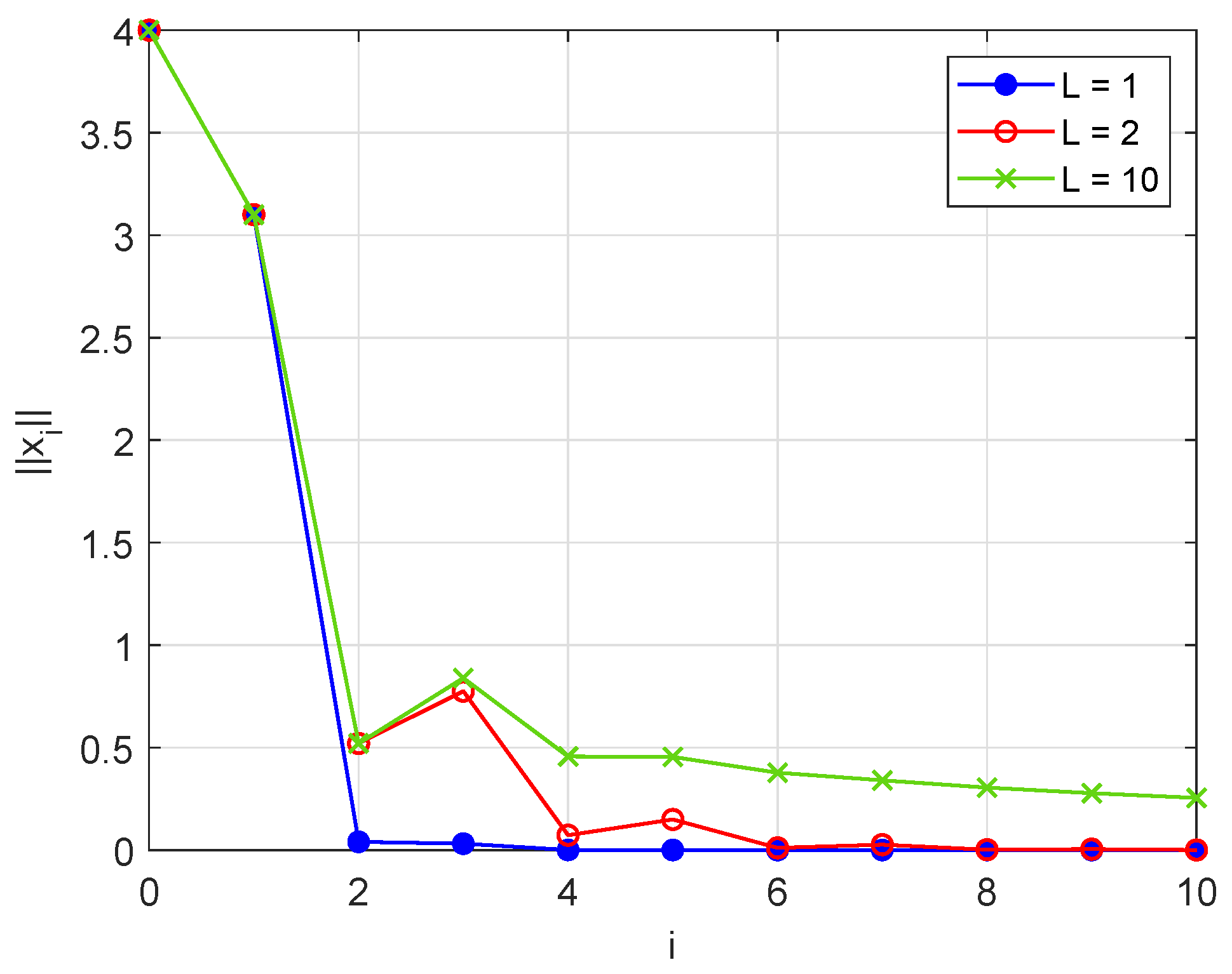
From (99) it follows that the considered system is practically superstable for $L=1$. The state vector norms for $x_0=\left[142\right]$ and different values of L are plotted in Figure 1. We can see the monotonic decrease only for $L=1$.

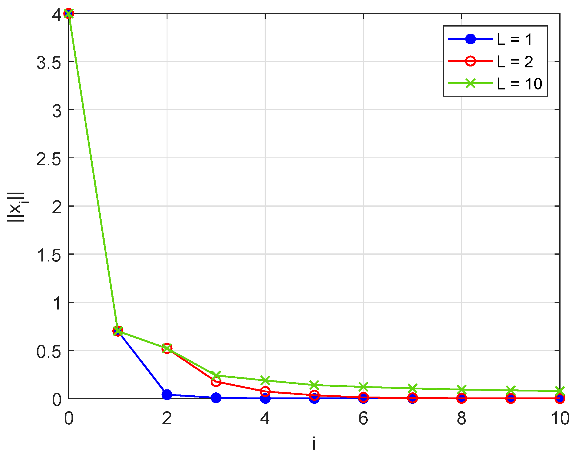
Now let us consider the SSF (60) with

$$\overline{K}=\left[\begin{array}{ccc}{k}_{11}& k_{12}& k_{13}\\ k_{21}& k_{22}& k_{23}\end{array}\right]$$

(100)

and

$$\begin{array}{c}\overline{K}\overline{E}{\overline{E}}^D=\left[\begin{array}{ccc}{k}_{11}& k_{12}+0.5k_{13}& 0\\ k_{21}& k_{22}+0.5k_{23}& 0\end{array}\right],\\ \overline{K}({\mathbb{I}}_3-\overline{E}{\overline{E}}^D)=\left[\begin{array}{ccc}0& -0.5k_{13}& k_{13}\\ 0& -0.5k_{23}& k_{23}\end{array}\right].\end{array}$$

(101)

Choosing $k_{13}=0$, $k_{23}=0$ yields $\overline{K}({\mathbb{I}}_3-\overline{E}{\overline{E}}^D)=0$. From (97) and

$$\overline{K}=\left[\begin{array}{ccc}0& 0& 0\\ 0& 1& 0\end{array}\right]$$

(102)

we have

$${\overline{A}}_{C1}={\overline{A}}_{1\alpha }-{\overline{B}}_1\overline{K}=\left[\begin{array}{ccc}0.1& 0.15& 0\\ 0& -0.1& 0\\ 0& -0.05& 0\end{array}\right],{\overline{A}}_{C2}={\overline{B}}_2\overline{K}=\left[\begin{array}{ccc}0& 0& 0\\ 0& 0& 0\\ 0& -1& 0\end{array}\right]$$

(103)

and from (72) ${\overline{F}}_C={\overline{A}}_{C1}$ for $\overline{G}=0$. The desired values of the norm $\parallel {\overline{F}}_C\parallel$ are also given by (99) since the superstability conditions of Theorems 7 and 8 depend only on the fractional order $\alpha$ of the system. Thus, we have

$$\begin{array}{c}\parallel {\overline{F}}_C\parallel =\parallel {\overline{A}}_{C1}\parallel =∥\left[\begin{array}{ccc}0.1& 0.15& 0\\ 0& -0.1& 0\\ 0& -0.05& 0\end{array}\right]∥=0.25,\\ \parallel {\overline{A}}_{C2}\parallel =∥\left[\begin{array}{ccc}0& 0& 0\\ 0& 0& 0\\ 0& -1& 0\end{array}\right]∥=1.\end{array}$$

(104)

Therefore, by Theorem 11 the DDFL system (1), (93) with $\alpha =0.4$ and the SSF (60), (102) is superstable (for $L\to \infty$) since $\parallel {\overline{F}}_C\parallel <0.4$ and $\parallel {\overline{A}}_{C2}\parallel \le 1$. The state vector norms for $x_0=[14-2]$ and different values of L are plotted in Figure 2. We can see the monotonic decrease in every considered case. Similar results can also be obtained for any $L>10$. The set of consistent initial conditions of the CL-DDFL system with SSF is different since from (75) for $i=0$ we have $x_0\in \mathrm{Im}({\mathbb{I}}_3+{\overline{A}}_{C2})\overline{E}{\overline{E}}^D$.

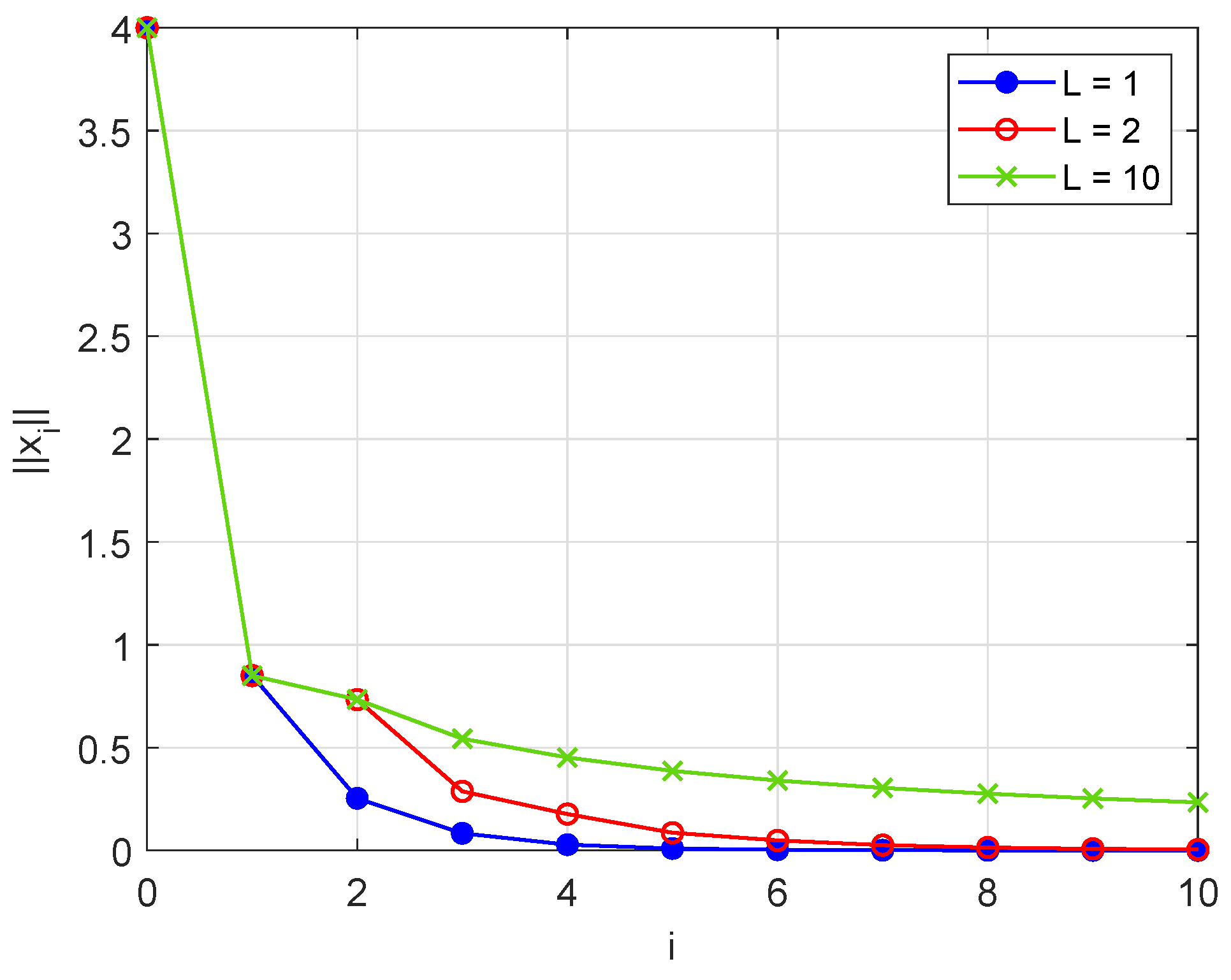
Finally, let us consider the DSF (79). In this case we cannot find the matrix H such that (88) holds since $\mathrm{rank}B=2$, $\mathrm{rank}[B{\mathbb{I}}_3-E]=3$ and the condition (89) is not satisfied. Using (83), (85), (93) and

$$H=\left[\begin{array}{ccc}0& 2& 2\\ 0& -2& 2\end{array}\right],K=\left[\begin{array}{ccc}0& 1& 0.125\\ 0& 0& 0\end{array}\right]$$

(105)

we obtain

$$A_C={(E+BH)}^{-1}(A-BK)=\left[\begin{array}{ccc}-0.3& 0.1& -0.0125\\ 0& -0.3333& 0.2917\\ 0& 0& -0.0625\end{array}\right]$$

(106)

and

$$A_{C\alpha }=A_C+{\mathbb{I}}_3\alpha =\left[\begin{array}{ccc}0.1& 0.1& -0.0125\\ 0& 0.0667& 0.2917\\ 0& 0& 0.3375\end{array}\right].$$

(107)

The norm of (107) is given by

$$\parallel A_{C\alpha }\parallel =∥\left[\begin{array}{ccc}0.1& 0.1& -0.0125\\ 0& 0.0667& 0.2917\\ 0& 0& 0.3375\end{array}\right]∥=0.3584.$$

(108)

Therefore, by Theorem 14, from (99) it follows that the DDFL system (1), (93) with $\alpha =0.4$ and the DSF (79), (105) is superstable (for $L\to \infty$) since $\parallel A_{C\alpha }\parallel <0.4$. The state vector norms for $x_0=\left[142\right]$ and different values of L are plotted in Figure 3. We can see the monotonic decrease in every considered case. Similar results can also be obtained for any $L>10$.

9. Concluding Remarks

In this article, the superstabilizing state-feedback control problem in DDFL systems with a regular matrix pencil has been studied. Methods for investigating the stability and superstability of such systems have been provided. Procedures for the computation of the SSF and DSF gain matrices such that the CL-DDFL system is superstable have been proposed. The main advantage of the presented approach is that it allows us to design the feedback control that affects pole-independent system properties such as superstability, for which the standard approach discussed in the literature is not applicable.

The main contributions of the article are as follows. A method for investigating the stability of DDFL systems based on the equivalent state-space model has been suggested (Theorems 4 and 5). Sufficient conditions for the superstability of DDFL systems have been provided (Theorem 9). Procedures for designing the SSF and DSF such that the CL-DDFL system is superstable have been proposed (Theorems 10, 11 and 14). The effectiveness of the presented approach has been demonstrated on a numerical example.

The sufficient conditions presented in the article were obtained through the use of many inequalities of matrix norms, which are easy to apply, but which do not give the exact result, e.g., from the inequalities (55) a noticeable overestimation may arise. An open problem is that of establishing the necessary superstability conditions of the considered class of dynamical systems.

This analysis can be further extended to fractional descriptor systems with different fractional orders.