Efficient Position Change Algorithms for Prolonging Driving Range of a Truck Platoon

Abstract

Cooperative automated driving technology has emerged as a potential way to increase the efficiency of transportation systems and enhance traffic safety by allowing vehicles to exchange relevant information via wireless communication. Truck platooning utilizes this technology and achieves synchronized braking and acceleration, controlling two or more trucks simultaneously. This synchronized control makes driving with a very short inter-vehicle distance among trucks possible and reduces aerodynamic drag. This provides significant fuel consumption reduction, both in leading and trailing trucks, and achieves fuel-saving improvement. However, the static positioning sacrifices trucks in the front since they consume more fuel energy because of more air resistance than the rears. To solve this in-equivalent fuel consumption reduction benefit, this paper presents several heuristic algorithms to balance fuel consumption reduction and prolong the driving ranges by exploiting position changes among trucks in a platoon. Furthermore, the proposed algorithms try to reduce the number of position changes as much as possible to prevent any fuel waste caused by the unnecessary position change operations. In this manner, each truck in the platoon is likely to share a similar fuel consumption reduction with fewer position change counts, thus addressing the challenge of in-equivalent fuel savings distribution and obtaining optimal fuel efficiency. Our extensive simulation results show that the proposed algorithms can prolong the total distance by approximately 3% increased in two-truck platooning and even higher in six-trucks platooning of approximately 8%. Moreover, our proposed algorithms can decrease the position change count and ensure that trucks only switch to position arrangement once with no duplicate. Therefore, truck platooning obtains the maximum driving range with fewer position change counts, thus achieving efficient fuel saving.

1. Introduction

Autonomous driving technology has significantly contributed to the automotive industry, where it promises the potential of improving safety and efficiency in the transportation system by reducing dangerous human driving behavior. This is based on the claim that 94% of crashes are caused by human errors [1]. While the number of vehicle traffic crashes is likely to rise consecutively, an autonomous vehicle becomes likewise one of the most intensively researched technologies to prevent such tragic accidents over the past decades. Furthermore, it also benefits many industries, including transportation and logistics, expecting to get positive impacts on cost reduction as it can decrease the cost of congestion and improve energy economy.

Truck platooning, one of the current widely known autonomous vehicle technologies, has continuously emerged in recent decades to address safety and sustainability issues in the transportation and logistic systems. This technology can be defined as a group of virtually synchronized trucks driving closely together in a single convoy. By using electronic coupling and wireless communications, it allows trucks to accelerate and decelerate simultaneously, thereby achieving driving with a small safety inter-vehicle space in which human drivers may not perform better. As a consequence of the small inter-vehicle distance, this significantly helps to improve fuel efficiency by reducing aerodynamic drag [2], which brings down fuel consumption and cuts optional costs. Several simulations-based studies [3,4,5,6,7] have proved that truck platooning results in fuel-saving approximately 10% on average, since air friction becomes a problem only for the leading truck such that it benefits trailing trucks with a much smaller resistance. Although previous experiments present diverse results due to different conditions [8], all results still validate that fuel efficiency can be improved the best in trailing trucks, providing much higher fuel saving compared to the lead one.

Even though truck platooning has already offered various benefits due to the lower fuel usage, we foresee that this technology can be improved to achieve a higher driving distance by changing the positions of the trucks within the platoon. The novel idea is based on the simple fact that trucks at the front consume more fuel energy than the rear trucks in the platoon. Thus, instead of having static positions during the entire driving, changing positions from time to time can redistribute the unequal fuel consumption rates evenly among the trucks. By exploiting such intuition, we have proposed preliminary position change algorithms in truck platooning [9]. The algorithms make trucks consume an almost similar amount of fuel by periodically changing the positions of trucks in the platoon until one runs out of energy. Theoretically, this algorithm allows truck platooning to drive longer because trucks with more fuel go to the front, where trucks with less energy can experience less air resistance at the rear positions. However, the results from our previous work [9] shows that the number of position changes is considered relatively high and may increase significant fuel consumption during the position change operations.

When considering the realistic scenario, one of the reasons for extra fuel consumption is an unsteady velocity caused by frequent acceleration and breaking. Even though the total driving range can be higher, one position change means trucks have to change their positions, thus wasting fuel energy in adjusting the velocity eventually. Our primary motivation is to maintain the maximum increased driving distance achieved with the position change methodology, yet with much less position change count.

In this paper, we mathematically formulate the position change problem as an optimization problem. Furthermore, the heuristic algorithms proposed in [9] are revised in a more rigorous manner so that they can be applied to more general cases. This paper also proposes an improved position change algorithm that promises a smaller number of position changes, achieving more efficient fuel-saving while still achieving the highest driving range. Basically, trucks with the higher remaining fuel capacity move to the front of the platoon such that all trucks arrange in descending order of fuel left. We notice that the position arrangement may have similar patterns over and over, since the platoon already shares fair fuel consumption. This urges us to reorganize the arrangement pattern where truck platooning only switches to each pattern once with no duplicates to reduce the number of position changes. The simulation-based evaluation shows that the number of position changes is significantly reduced compared to the original algorithm. Thus, it can significantly decrease fuel costs per freight transportation, thus enhancing fuel economy and providing much more traffic efficiency. To the best of our knowledge, our work is the first to bring position change methodology into truck platooning technology.

The contributions of the paper can be summarized as follows.

• We formulate the position change problem as an optimization problem in a more rigorous manner. We define the assumptions and the objects more clearly.
• We revise two previously proposed position change algorithms based on the formulated optimization problem.
• We propose a new objective, which is the number of position changes, and a new heuristic algorithm for the new objective.

The rest of the paper is organized as follows. In Section 2, we describe the background and review the related works. Section 3 proposes several heuristic position change algorithms, which focus on prolonging the driving range and reducing the number of position changes. We present the evaluation results of the proposed algorithms in Section 4, and discuss the computational complexity in Section 5. Lastly, the paper is concluded in Section 6.

2. Literature Review

Several research institutions and transportation manufacturers have eagerly studied and developed truck platooning technologies for decades, expecting a fully automated vehicle in the current timeline and bringing human beings a brighter future in the freight industry and transportation system. According to the levels of driving automation by SAE International [10], Level 5 or full automated refers to full driving automation, where vehicles automatically pilot themselves in all driving environments with no human driver required. Still, truck platooning realizes only SAE level 2 automated driving, where trucks are allowed to control both steering and acceleration/deceleration capabilities, yet the driver is needed and makes it fall short of self-driving automation. An effort aims to address challenges to accomplish platooning systems for higher automation levels, as well as ascertaining solutions to enhance fuel efficiency. Several studies have proved the benefits of reduced aerodynamic phenomena. However, vehicle configurations and other subject influencing factors are needed to be studied to achieve optimal fuel savings in the platoon. For example, the following questions should be addressed.

• What are the influencing factors on fuel consumption reduction in the truck platooning system?
• What are optimal configurations of trucks to get the highest fuel savings?
• Does vehicle position in the platoon affect fuel consumption for each truck? If yes, how does it remarkably influence the fuel consumption reduction in each position?

Many papers have been studied to answer the above questions. In early 2000, Bonnet et al. [4] conducted two-truck platooning experiments with heavy-duty ACTROS semi-trailer trucks. The lead truck is driven manually, and the trailing truck is operated automatically with a driver assistance system. Two measurement tests were carried out with two constant velocities of 80 km/h and 60 km/h and inter-vehicle distances from 5 m up to 16 m. The trailing truck experienced a remarkable fuel consumption reduction of 21% at 80 km/h velocity with 10 m longitudinal spacing, and the leading truck experienced a 7% reduction in the corresponding configurations. The demonstration results further show that both velocity and inter-vehicle distance significantly impact the fuel consumption reduction where the decreasing gap space makes reduction benefits increase, whereas decreasing speed makes the opposite outcomes. It should also be noted that the leading truck can also have fuel reduction in platooning compared to that case of driving alone.

A platoon of three tractor–trailer truck experiment was conducted under automated longitudinal platoon control by Lu et al. [5] in 2011. Besides the environmental conditions, they considerably investigate the effects of the position within the platoon and the inter-vehicle spacing. With three heavy trucks at 85 km/h speed and a gap spacing of 6 m, the third truck saves the most fuel among the three, and the second still achieves more fuel-saving than the first truck. To be specific, the leading truck achieves 4.3% of reduction in fuel consumption, and about 10% and 14% fuel savings are achieved for the second and the third truck, respectively.

The aerodynamic simulation in a two-truck platooning by Dávila et al. [6] has been carried out to select the most appropriate gaps between the platoon in 2013. This work consists of a series of CFD (Computational Fluid Dynamics) simulations from 3 m to 15 m gap spacing configurations, considering steady environmental conditions at 90 km/h velocity. The results show that trucks in the platoon remarkably achieve fuel-saving approximately from 7% to 15% at 8 m inter-vehicle distance, and about only 2% to 11% fuel saving at 15 m. This work also confirms that the fuel consumption can be reduced with the shortened gap spacing.

Lammert et al. [7] evaluated a two Class 8 tractor–trailer platoon on fuel consumption in 2014. The experiments were carried out with a steady-state speed from 55 mph to 70 mph or approximately 88 km/h to 113 km/h, with inter-vehicle gaps ranging from 20 ft to 75 ft or about 6 m to 23 m, and the total gross vehicle weights (GVW) of 65,000 lbs and 80,000 lbs. According to the experimental results, significant fuel savings can be achieved for both leading and trailing trucks where the first truck experienced up to 5.3% of fuel-saving, and the second truck experienced up to 9.7% fuel-saving. The best configuration is 88 km/h constant velocity, roughly 9 m inter-vehicle distances, and 65,000 GVW, which results in 6.4% fuel consumption reduction in the whole convoy. They further conclude that atmospheric conditions and heavy loads of trucks may significantly influence in savings attainable, considering heavily loaded vehicles consume fuel at a higher rate because of the increased airflow.

Truck platooning system experiments and studies have been summarized through Zhang et al.’s work [8] in 2020. The longitudinal space is considered the highest influencing factor in truck platooning fuel economy. The position and vehicle configurations are also made to the top-tree highest respectively. In summary, the overall performance of fuel consumption reduction in a platoon can be increased with closer longitudinal space. The vehicle’s position in the platoon influences fuel consumption in the way that trailing vehicles always experience more fuel savings and even more in next-order trucks due to the less aerodynamic drag. Masses and loads also significantly affect the percentage of fuel savings in the platoon, as the heavy loads consume fuel much more than the ordinarily loaded or empty trailer trucks.

All of the previous studies that we have discussed so far come to the conclusion that influencing factors such as longitudinal spacing, a vehicle position in a platoon, and vehicle configurations, affect the effectiveness of energy-saving in the truck platooning system. These factors influence the reduction of aerodynamic drags, thereby achieving reduced fuel consumption consistently. Nevertheless, experimental tests conducted under different conditions can cause different results, where the optimal solution for truck configurations cannot be determined. This is because it depends on various uncontrollable conditions, including road grades, presences of traffic, and weather conditions, which are restricted in reality. Still, these studies help us understand the influence of positions in a platoon on the unequal distributions of fuel consumption reduction, thus urging us to address the remaining challenge to improve fuel efficiency optimally.

In our previous work [9], we have introduced the position change problem, of which the objective is to prolong the driving range with the given amount of initial fuel. We have also proposed two heuristics (“Fuel Amount Heuristic (FAH)” and “Traveling Time Heuristic (TTH)”) for the position change problem to enable the platoon to drive as far as possible and reach the maximum driving range or distance, thus enhancing fuel-saving the most. The difference between the two heuristics is the conditions when the vehicles should change their positions. In “Fuel Amount Heuristic”, the platoon starts in the order of the initial fuel amount of the trucks. For any two adjacent vehicles, if the remaining fuel of the leading truck is less than the remaining fuel of the trailing truck by more than a threshold c, then the two vehicles should change their position. The intuition is that we want to put a vehicle with more energy into the front positions, but not so frequently. In the “Traveling Time Heuristic” algorithm, we first divide the time into multiple time slots. At the beginning of each time slot, the truck with the highest fuel moves to the front of the platoon and the second-highest moves to the second position, and so forth. Eventually, the platoon forms a descending order arrangement in each time slot and is ready for the next position changes until one of the trucks runs out of fuel. However, Ref. [9] only provide preliminary results of the proposed heuristic algorithms, and the description of the problem is not rigorous. Furthermore, they do not explicitly focus on the problem of frequent position changes.

3. The Position Change Problem and the Algorithms

In this section, we first formally define the position change problem. We need to clarify the input and output of the problem and the objective of the problem. Then, we combine the previously proposed two heuristic algorithms into a unified one and refine the description of the unified algorithm. Finally, we introduce a new objective of the position change problem, which is to minimize the number of position changes, and propose a new heuristic algorithm for this new objective.

3.1. Formulation of the Position Change Problem

A longitudinal formation with a very close inter-vehicle spacing allows the platooning technology to reduce aerodynamic drag, reducing the fuel consumption since a quarter of the fuel consumption is caused by air drags [11]. However, each truck has an unequal distribution of fuel consumption reduction depending on its position in the platoon. For example, the first truck in the platoon has the highest fuel consumption rate among the convoy. This may lead to the situation where the platoon needs to stop to refuel the trucks more often, which increases wasted time. Hence, we see the potential in improving the effectiveness of fuel energy by making the fuel consumption rates of the trucks to be balanced as much as possible, thus achieving a longer driving distance in total since all the fuel in each truck can be consumed efficiently.

Since the leading truck experiences aerodynamic drag the most and delivers the highest fuel consumption compared to the other trucks in the platoon, we ensure that trucks with more fuel should move to the front to encounter the extra air resistance while still holding the higher amount of fuel. Similarly, trucks with less fuel should move to the trailing positions where they can experience less aerodynamic drag and obtain a lower rate of fuel consumption. By changing positions periodically, the truck platooning is likely to manage a balanced amount of fuel along traveling, such that the longer total driving range can be achieved compared to the platoon without any position change. Both the two heuristic algorithms (“FAH” and “TTH”) proposed in [9] try to follow this intuition.

To achieve the longest driving distance, the threshold c of “FAH” and the time slot size $\delta$ of “TTH” should be very small. In other words, the platoon needs to change the positions whenever the ordering is not the same as the ordering of the number of fuels. Thus, theoretically, the two heuristic algorithms are the same when c and $\delta$ are very small, in which the order of the vehicles in the platoon is the order of remaining fuels at any instant. In the following, we formulate the position change problem by using the concept of time slots introduced in the “TTH” algorithm. We first define some notations in

Table 1. Notations.

Notation	Definition
V	Set of n vehicles in a platoon, i.e., $\{1,2,...,n\}$
$t_k$	Starting time of the time slot $k(\ge 0)$. The time is divided into multiple time slots. The length of each time slot is $\delta (=t_{k+1}-t_k)$.
$P(i,k)$	Position of a vehicle i at time slot k. P is the position change matrix.
$F_i\left(t\right)$	Fuel amount of a truck i at time t
$F\left(t\right)$	Set of remaining fuels of n trucks at time t, i.e., $\{F_1\left(t\right),F_2\left(t\right),...,F_n\left(t\right)\}$
r	Steady fuel consumption rate per unit distance
$g\left(j\right)$	Fuel consumption reduction rate at a truck position j, $1\le j\le n$. Lower position number means a front position in the platoon
s	Speed of the vehicles in the platoon

.

We assume that $g\left(j\right)\ge g\left(i\right)$ for any two positions i and j where $j>i$. It should be noted that $j>i$ means that the position i is in the front compared to the position j. Thus, this assumption means that front positions have a smaller consumption reduction rate than rear positions. In other words, a vehicle at position i consumes more fuel than at position j. Considering the fuel consumption reduction rate, the fuel amount at time $t_{k+1}$, i.e., $F_i\left(t_{k+1}\right)$, is given as follows:

$$\begin{array}{ccc}\hfill F_i\left(t_{k+1}\right)& =& F_i\left(t_k\right)-r\times (1-g\left(P(i,k)\right))\times (t_{k+1}-t_k)\times s\hfill \end{array}$$

(1)

$$\begin{array}{ccc}& =& F_i\left(t_k\right)-r\times (1-g\left(P(i,k)\right))\times \delta \times s\hfill \end{array}$$

(2)

In the above equations, $\delta \times s$ is the distance that a truck travels in a time slot. Since r is the fuel consumption rate per unit distance, the amount of fuel consumed in a time slot is $r\times \delta \times s$ in a non-platoon driving. However, due to the platooning effect, the fuel consumption is reduced by $(1-g(P(i,k)\left)\right)$ in such a way that when $g\left(P\right(i,k\left)\right)$ increases, the platoon has less fuel consumption. The set of initial amount of fuel at the beginning of driving is $F\left(0\right)=\{F_1\left(0\right),F_2\left(0\right),...,F_n\left(0\right)\}$.

The platoon needs to stop driving when a truck has empty fuel. Thus, if the fuel of any truck i becomes empty in a time slot K, i.e., $F_i\left(t_K\right)\ge 0$ and $F_i\left(t_{K+1}\right)<0$, then the longest driving range of the platoon is $K\times \delta \times s$. The objective of the problem is to produce a position change matrix P that achieves the longest driving range with the given set of the initial amount of fuels, $F\left(0\right)$, and the time slot size $\delta$. The optimization problem of position changes can be expressed as follows.

$$\begin{array}{cccc}\hfill & \underset{P(i,k)}{\mathrm{maximize}}\hfill & \hfill & K\hfill \\ \hfill & \mathrm{subject}\mathrm{to}\hfill & \hfill & t_0=0\hfill \\ \hfill & \hfill & & t_{k+1}=t_k+\delta ,k\ge 0\hfill \\ \hfill & \hfill & & F_i\left(t_k\right)\ge 0,\mathrm{for}i\in V,0\le k\le K\hfill \\ \hfill & \hfill & & F_i\left(t_{k+1}\right)=F_i\left(t_k\right)-r\times (1-g\left(P(i,k)\right))\times \delta \times s,\mathrm{for}0\le j\le K\hfill \\ \hfill & \hfill & & P(i,k)\in \{1,...,n\},\mathrm{for}i\in V\hfill \\ \hfill & \hfill & & P(i,k)\ne P(j,k),\mathrm{if}i\ne j\mathrm{for}i,j\in V\hfill \end{array}$$

Our primary objective is to maximize the number of time slots, K, while maintaining the remaining amount of fuels $F_i\left(t_k\right)$ non-negative. In other words, we want to increase the driving range. The variables in the above optimization problem are $P(i,k)$, which is the position of a vehicle i at time slot k. By changing the values of $P(i,k)$, we have different objective values K. There can be some remaining fuel in the vehicles, which is not enough for the next time slot. However, we ignore it and only consider the number of time slots that can be driven entirely because when $\delta$ is small, the remaining fuel becomes very small.

Now, we rigorously define “Traveling Time Heuristic” by using the notations defined in Table 1. “TTH” is described as in Algorithm 1. It can be easily proved that the proposed algorithm produces an optimal position sequence $P(i,k)$ for all the vehicles in the platoon in the sense that it produces the longest driving range. Furthermore, when $\delta$ goes to zero, we achieve the highest driving range possible because the platoon does not have any remaining fuel. It means that the platoon driving stops when one of the trucks has exactly zero fuel remaining.

Next, we discuss some properties of “TTH”. First of all, a simple lower bound and an upper bound of the driving range of the platoon can be constructed as follows. If the truck with the smallest initial fuel drives in the leading position all the time, the fuel depletes earliest, and the corresponding distance is given by Equation (3). Similarly, an upper bound is a case when the truck with the most initial fuel drives at the end of the platoon, and the distance is given by Equation (4).

$$\begin{array}{cc}\hfill \mathrm{a\; lower\; bound}:& \frac{min\left\{F\right(0\left)\right\}}{r\times (1-g(1\left)\right)}\end{array}$$

(3)

$$\begin{array}{cc}\hfill \mathrm{an\; upper\; bound}:& \frac{max\left\{F\right(0\left)\right\}}{r\times (1-g(n\left)\right)}\end{array}$$

(4)

Another thing is about the differences in the amount of fuels of the vehicles. “TTH” tries to reduce the differences in the amount of fuels of the vehicles. Theoretically, when the initial amounts of fuels are equal for all the vehicles, by applying “TTH”, the difference among the fuels at the any time slot is bounded by $r\times \delta \times s\times \left(g\right(n)-g(1\left)\right)$. The derivation of this amount is given at Lemma 1. The proof is given at the Appendix A.

Algorithm 1: Traveling Time Heuristic.

Input: V, $F\left(0\right)$, $\delta$  Output: P  V: the set of vehicles  $F\left(0\right)$: Initial fuel amounts at $t=0$, i.e., $F\left(0\right)=\{F_1\left(0\right),F_2\left(0\right),...,F_n\left(0\right)\}$  $\delta$: Size of each time slot  P: Positions of the vehicles at each time slot  $t\leftarrow 0$  $k\leftarrow 0$  while $F_i\left(t\right)>0$ for all i do   Sort the vehicles by their remaining fuel $F_i\left(t\right)$ in decreasing order   $c\left(i\right)$: the position of the vehicle i in the sorted list   for each vehicle $i\in V$ do    $P(i,k)\leftarrow c\left(i\right)$    /* calculate fuel amount at the next time slot */    $F_i(t+\delta )\leftarrow F_i\left(t\right)-r\times (1-g\left(P(i,k)\right))\times \delta \times s$   $t\leftarrow t+\delta$   $k\leftarrow k+1$  return P

Lemma 1.

When the initial amounts of fuels are equal for all the vehicles, by applying “TTH”, the difference among the fuels at time $t_k$ is bounded by $r\times \delta \times s\times \left(g\right(n)-g(1\left)\right)$ for $k\ge 0$.

It should be noted that the largest difference occurs after the time slot that starts with the equal amount of fuels for all the cars. For example, suppose that at $t_0$, all the fuel amounts are equal to x. Then, at time $t_1$, the first truck of the time slot 0 has fuel amount of $a_1^{\prime }=x-r\times \delta \times s\times (1-g\left(1\right))$ and the nth truck of the time slot 0 has fuel amount of $a_n^{\prime }=x-r\times \delta \times s\times (1-g\left(n\right))$. So the largest fuel difference at time $t_1$ is $(a_n^{\prime }-a_1^{\prime })=r\times \delta \times s\times (g\left(n\right)-g\left(1\right))$.

3.2. Reduction of Position Changes

As noted before, if we decrease $\delta$, the vehicles need to change their position within the platoon more frequently. Since the position change operation needs a change of speed of vehicles, which might cause extra consumption of fuel, it is very desirable to reduce the number of position changes. To address this ongoing problem, we turn our focus to reducing the number of position changes while achieving the same driving range as before.

The intuition of reduction in the number of position changes comes from the position change matrix P. For two time slot ids $k_1$ and $k_2$, if $P(i,k_1)=P(i,k_2)$ for all $i\in V$, we swap the time slot $k_1+1$ or $k_1-1$ with the time slot $k_2$. Thus, two consecutive time slots maintain the same position orders, which reduces the position change for the two time slots. As an example, let us consider a position change matrix P shown in

Table 2. A position change matrix P.

P		k
		0	1	2	3	4
i	1	1	2	3	1	2
	2	2	1	2	2	1
	3	3	3	1	3	3
	4	4	4	4	4	4

.

In this example, the number of vehicles is $n=4$ and the number of time slots is 5. There are same patterns of position arrangements when $k=0$ and $k=3$, and $k=1$ and $k=4$. In this case, we can reorder the time slots so that we have

Table 3. A reordered position change matrix P’.

P’		k
		0	1	2	3	4
i	1	1	1	2	2	3
	2	2	2	1	1	2
	3	3	3	3	3	1
	4	4	4	4	4	4

, which may have fewer position changes.

Before we discuss the algorithms to reorder a position change matrix, we need to define the definition of position changes. We come up with two different definitions of position changes. One way is to count the position changes vehicle-wise. When there is any position change for a vehicle in the platoon, every position change is counted as one change. For example, in Table 3, the positions of vehicle 1 changes from 1 to 2, and 2 to 3. Thus, vehicle 1 has two position changes. Similarly, vehicles $2,3$, and 4 have $2,1,0$ position changes, respectively. So the total number of position changes is 5.

Another way is to count the position changes time slot-wise. It is considered as one position change only if there is any position difference between two consecutive time slots. In Table 3, we only have two position changes: one between $k=1$ and $k=2$, and the other between $k=3$ and $k=4$. In this paper, we use the time slot-wise definition where it has only two position changes from $k=1$ to $k=2$ and from $k=3$ to $k=4$ in Table 3, compared to the case of Table 2, which has four position changes.

So the remaining question is how to find a good reordering of time slots of P. We propose a simple sort based algorithm called “Sorted Time Slot (STS)”. STS sorts the columns of P, which is generated by running the algorithm TTH described in Algorithm 1, in lexicographical order. The sorting operation in STS results in moving duplicate columns into consecutive columns, thus reducing the number of position changes. Actually, Table 3 is derived by running STS for the position change matrix P in Table 2. Since the algorithm is quite simple and intuitive, we do not elaborate further.

4. Performance Analysis and Simulation Results

In this section, we evaluate the performance of the heuristic algorithms that we have proposed: “Fuel Amount Heuristic (FAH)”, “Traveling Time Heuristic (TTH)”, and “Sorted Time Slot (STS)”. The performance metrics that we focus in this section are the total driving range and the number of position changes. Position change operation helps save the fuels of the trucks participating in the platoon by exploiting FAH and TTH. Furthermore, “STS” aims to reduce the number of position changes.

To simulate the algorithms in a more realistic environment, we first define some parameters used in the algorithms. The trucks are driving at the constant speed of s = 85 km/h and inter-distance spacing at 6 m, as it presents the most reliable longitudinal spacing that may provide the highest fuel-saving. Each truck exhibits the same fuel consumption rate at r = 32.6 L/100 km, which is known as the average EU tractor–trailers [12], and starts with the same amount of initial fuel of 300 gallons or 1135.62 L, i.e., $F_i\left(0\right)$ = 1135.62 L for all $i\in V$. We assume that there is no fuel consumption in the process of the position change. Furthermore, we also assume that there is no road or load-related fuel consumption. For the fuel consumption reduction parameter $g\left(i\right)$, we use the results studied by Lu et al. [5]. Thus, we set $g\left(1\right)=4.3\%$, $g\left(2\right)=10\%$, and $g\left(3\right)=14\%$. We further assume that from the fourth position and after, the consumption reduction rates are the same as 14%, i.e., $g\left(i\right)=14\%$ for $i\ge 3$, since there is no available information about the reduction rates after the third position in the existing literature.

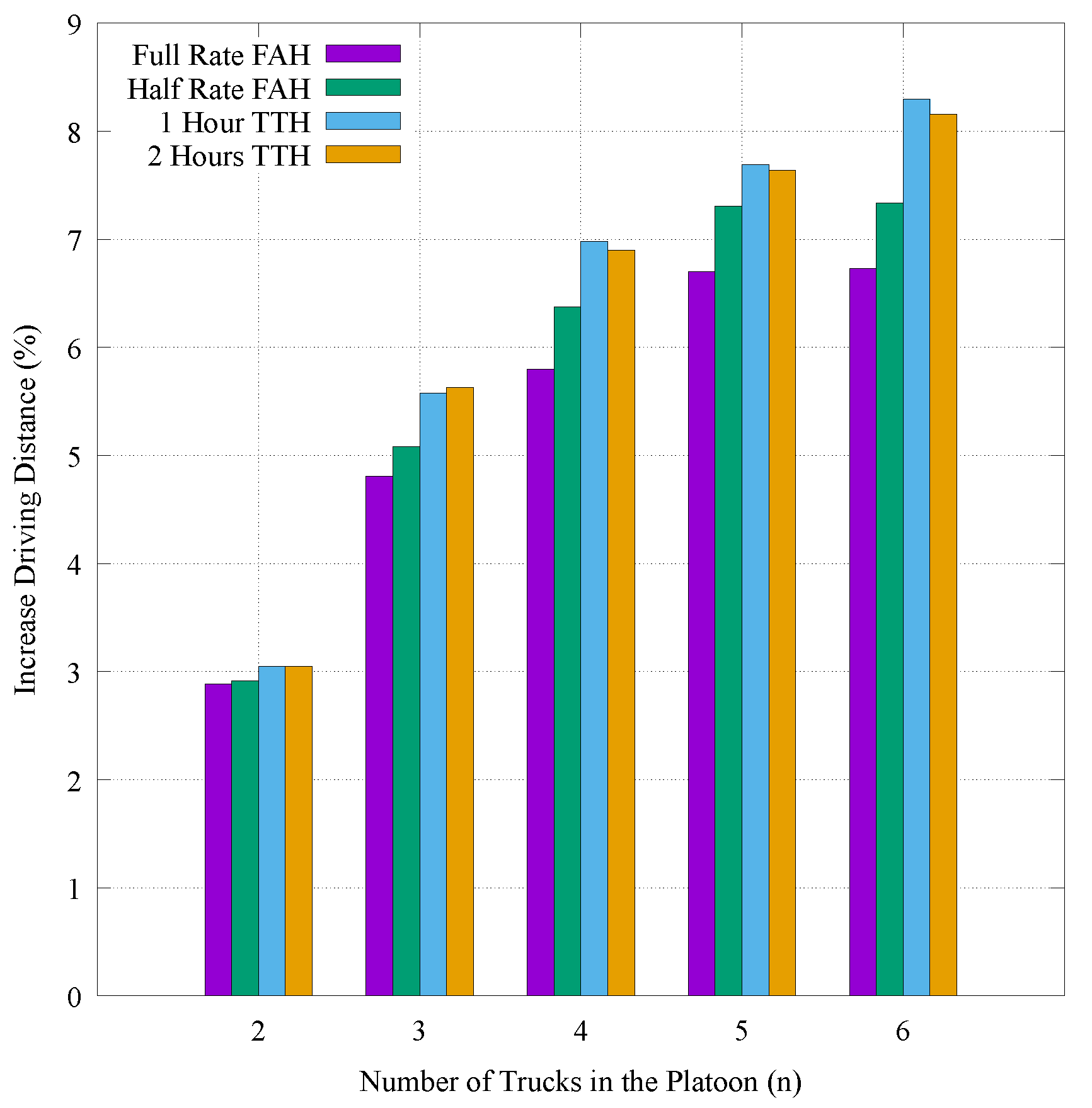
Figure 1 shows the increased driving distance compared to the fixed order truck platooning in percentage over a various number of trucks. For “Fuel Amount Heuristic (FAH)”, we set c with two different values. The first is to set c as an amount of fuel needed for 100 km traveling, based on fuel consumption rates, called “Full Rate”. The second one is to set c as the amount of fuel needed for 50 km traveling, called “Half Rate”. For “Traveling Time Heuristic (TTH)”, we set $\delta$ to 1 h and 2 h. We vary the number of trucks n from 2 to 6. The values of parameters used in this simulation are summarized in

Table 4. Simulation Parameters.

Parameter	Value	Unit
n: number of trucks in the platoon	2, ..., 6	-
s: velocity	85	km/h
r: consumption rate	0.326	L/km
$F_i\left(0\right)$: initial fuel at position i	1135.62	L
$g\left(i\right)$: fuel consumption reduction rate at truck position i	4.3%; $i=1$ 10%; $i=2$ 14%; $i\ge 3$	-
$c_1$: threshold of “Full Rate”	32.6	L
$c_2$: threshold of “Half Rate”	16.3	L
${\delta }_1$: time slot size of “1 Hour”	1	h
${\delta }_2$: time slot size of “2 Hours”	2	h

.

Since the initial fuel amounts are the same, the fixed order positioning represents the lower bound of the driving range. The comparative simulation result shows that changing vehicle positions by the proposed algorithms increases the cumulative fuel consumption reduction within the platoon, making the total driving range much longer with the same initial fuel capacity. Furthermore, it indicates that the higher the number of trucks in the platoon, the longer the driving distance. To be specific, the percentage of the increased range rises from approximately 2.8–3.0% in two-truck platooning to 6.7–8.1% in six-truck platooning. The result is justified by the concept of average reduction rates of n trucks. The operation of changing positions is to make the reduction rates of the trucks similar. In other words, the average reduction rate of the n trucks becomes $\frac{{\sum }_{j=1}^{n}g\left(j\right)}{n}$. Since $g\left(j\right)$ is larger for a larger j, the average reduction rate increases as n increases. Therefore, we have longer driving ranges.

Compared to Lu et al.’s work, since there are no position changes, the maximum fuel consumption reduction rate remains steady with the first truck position at 4.3% no regards the number of trucks in the platoon. Meanwhile, our proposed algorithm can obtain a higher fuel consumption reduction rate. For example, $\frac{4.3\%+10\%}{2}=7.15\%$ for two-truck platooning.

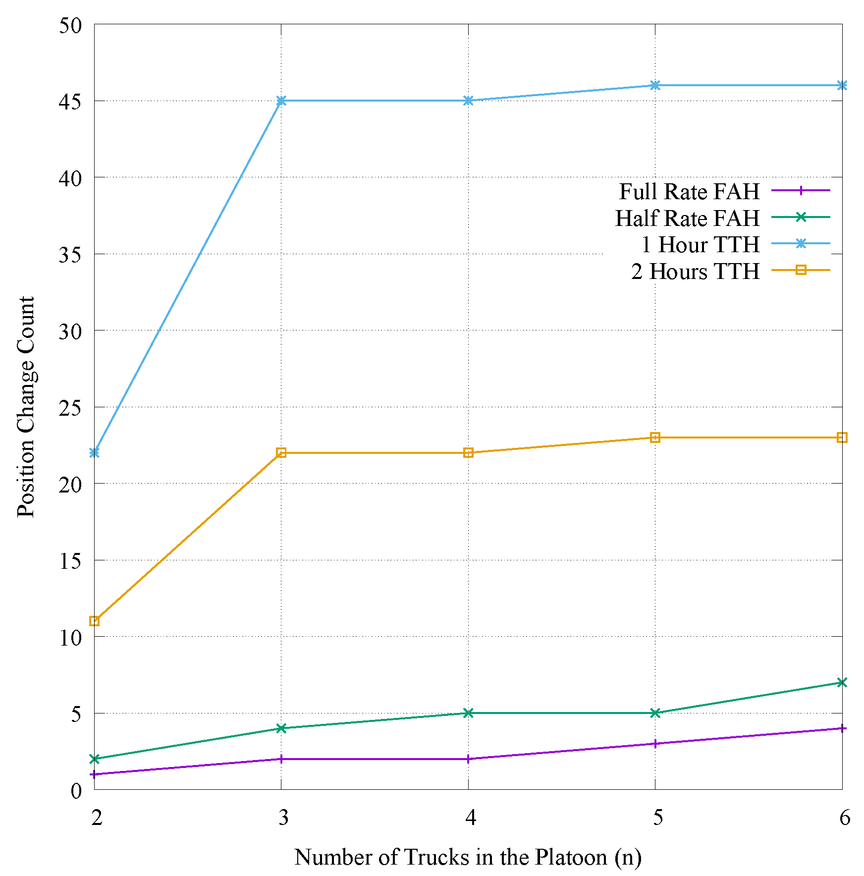
For the same simulation, Figure 2 shows the number of position changes in the platoon. Before analyzing the result, we first compute the driving range and driving hour without platooning. The driving range without platooning is $F_i\left(0\right)/r$ = 1135.62 L/(32.6 L/100 km) = 3483 km. Since the speed of the trucks is s = 85 km/h, the driving time is about 41 h. Due to the effect of position changes, the driving range and time become longer than those values. In Figure 2, FAH shows very few numbers of position changes, and TTH shows a high position change count. The reason is quite clear. In FAH, the position change occurs when the difference of the fuels of two consecutive trucks becomes larger than the fuel amount of 100 km driving, i.e., 32.6 L. For a simple calculation, we consider $g\left(1\right)$ and $g\left(2\right)$. The reduction rate difference is $5.7\%=\left(g\right(2)-g(1\left)\right)$. Thus, it takes 100 km/0.057 = 1754 km of driving to create this much fuel difference. Considering the speed of the trucks s = 85 km/h, it takes about 20 h. Thus, the position change happens 2 or 3 times the total driving. This count is for the first and second trucks. There are position changes at other positions, too. So it is quite reasonable to have 5 position changes when $n=4$ for Full Rate FAH.

Regarding the results of TTH, we have 22 time slots for $\delta =$ “1 Hour” at $n=2$. The count rises to approximately 46 rounds when $n\ge 3$. This number is quite reasonable considering the analysis of the driving time. Since the total driving time becomes more than 41 h due to the position changes, when $\delta$ = 1 h, we should have more than 41 position changes during the platooning. Similarly, position changing every “2 Hours” shows half of the “1 Hour” total number of position changes for each n.

One question is why we have only half of the position changes at $n=2$ compared to that of $n=3$. The reason is quite straightforward. When $n=2$, at every 2 h, the fuels of the two trucks become the same so that there is no need to change the positions, which results in half of the expected position changes. However, for $n\ge 3$, this is not the case. For example, when $n=3$, suppose that in the first time slot, we have sequences $(1,2,3)$. Then, in the second time slot, we should have the sequence of $(3,2,1)$. At the end of the second time slot, truck 1 and 3 have the same amount of fuel, but not truck 2. After the third time slot, there is no way to make the fuels of the three trucks the same. Therefore, for $n\ge 3$, we have a similar number of sequence changes to the driving hours.

Based on the simulation results so far, it is clear that if we increase $\delta$ in TTH, we have a lower driving range and lower switching counts. Similarly, if we decrease $\delta$, we have a higher driving range and a higher number of position changes. “Sorted Time Slot (STS)” helps reduce the position change counts while having the same driving range as TTH.

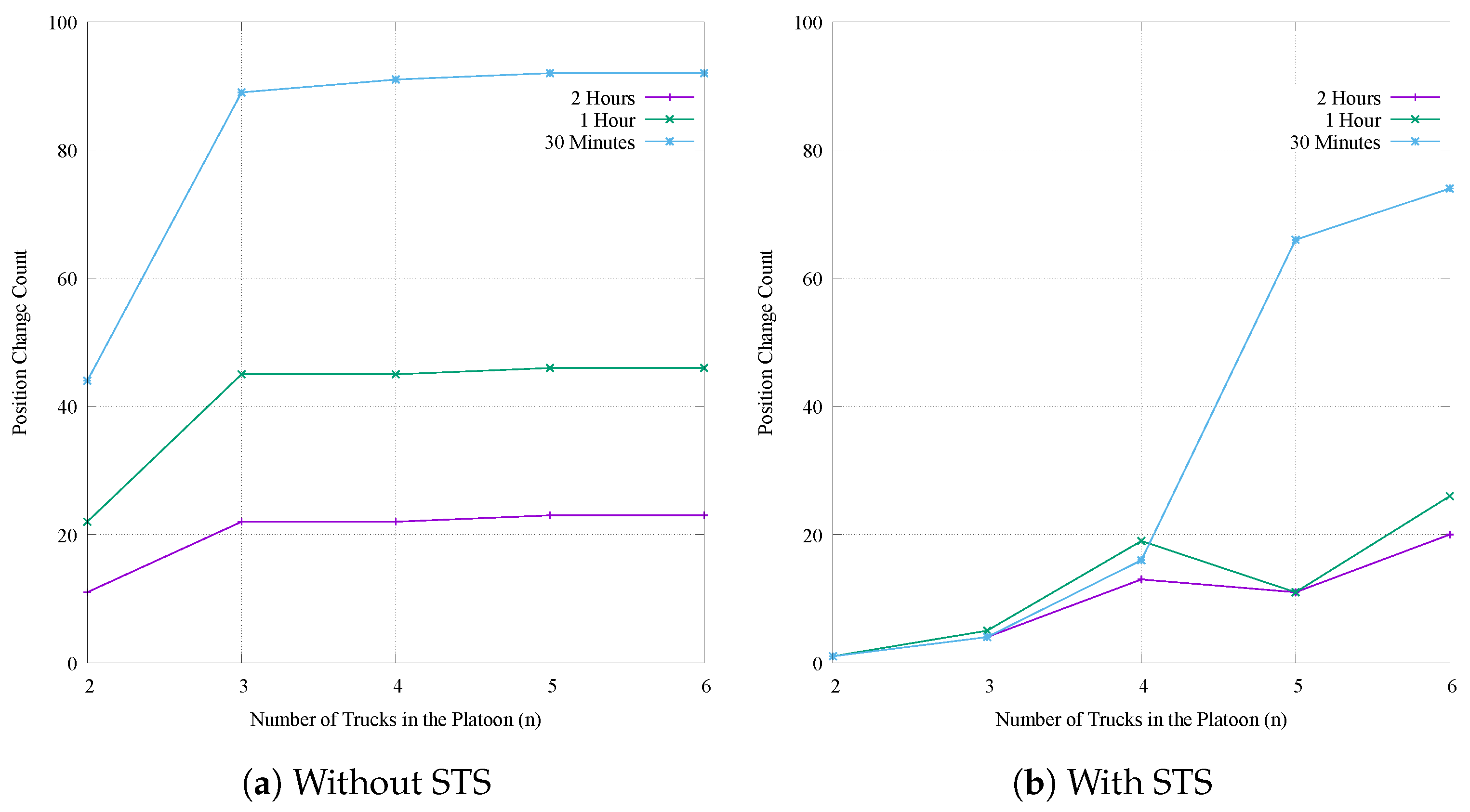
Figure 3 shows the comparison of sequence changing count with and without STS over the number of trucks. For the case without STS shown in Figure 3a, the results are the same as that of Figure 2. Theoretically, there can be $n!$ different position combinations. Then, the maximum number of position changes is $n!-1$. However, not all the cases appear in the positions because the number of time slots is much less than $n!$. Furthermore, there can be many duplicates in multiple time slots. Thus, sorting the time slots may reduce the number of position changes because we can rearrange the time slots so that duplicates join together. Figure 3b shows the switching counts with STS. It can be clearly seen that the number of position changes is much less for various time slot sizes $\delta$. Furthermore, we achieve the optimal position change count for $n=2$, which is just one, while still holding the longest driving distance. When $n=2$, the position change matrix P has columns of $(1,2)$ or $(2,1)$. In STS, we sort the position change matrix by their columns, so we have only one position change from $(1,2)$ to $(2,1)$.

The maximum number of unique position sequences for n trucks is $n!$. For example, $6!=720$. However, in Figure 3b, we have less than 80 counts for $n=6$. That is because we have only around 100 time slots when $\delta =30$ min. If there are more time slots, then we have more combinations of position sequences, thus many position changes. To see the effect of varying $\delta$, we also conduct the simulation under shorter $\delta$ from 10 to 60 min each is 10 min apart. 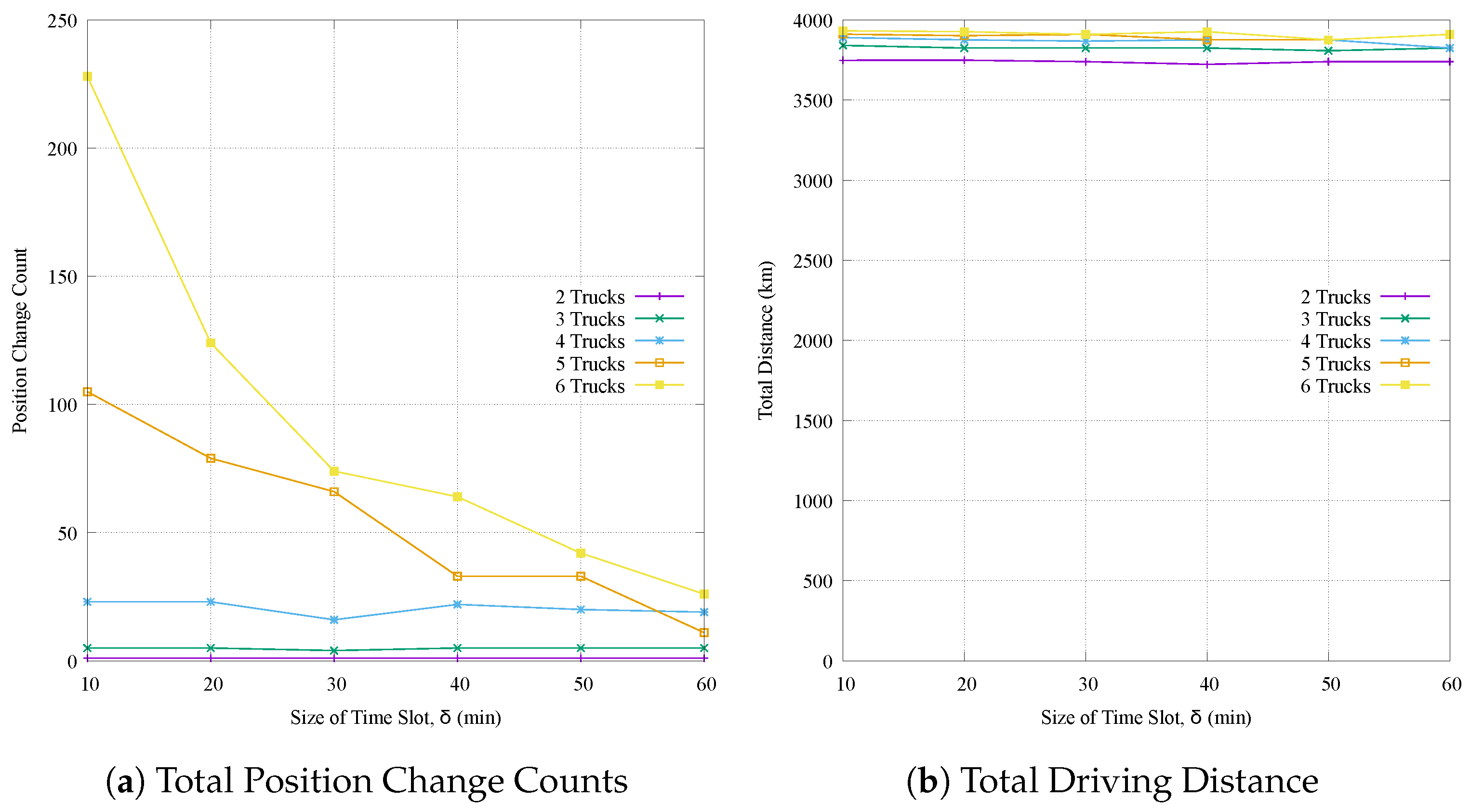Figure 4a shows the number of position changes over various $\delta$. A shorter time slot increases the number of time slots for the same amount of initial fuel. As we can expect, a smaller $\delta$ shows a higher position change count. This shows a trade-off between the number of position changes and the total driving range (distance).

To analyze the trade-off, we compute the total driving distances over $\delta$. Figure 4b shows the results. Interestingly, the total distances do not differ much for different $\delta$. The results are quite contrary to our intuition. Therefore, we further analyze the results. The case with $\delta =10$ and $n=2$ has 264 time slots to drive, and the remaining fuels are the same as 3.55566 L, which is not enough for the next 10 min time slot. Actually, $264=2^3\times 3\times 11=6\times 44$. Thus, 264 time slots for $\delta =10$ is 44 times slots for $\delta =60$. It means that for $n=2$, the two cases of $\delta =10$ and $\delta =60$ show the same driving distance and have same residual fuel of 3.55566 L. This is somewhat coincidental due to the specific initial amount of fuel. On average, for a time slot size $\delta$, there can be residual amount of fuels enough to drive for $\delta /2$ amount of time. Thus, if s = 85 km/h, then the average driving distance difference between $\delta =10$ and $\delta =60$ is about 40 km. Nonetheless, since the proposed algorithms try to reduce the differences in the fuels among the trucks, the distance difference may not be large regardless of the time slot size $\delta$.

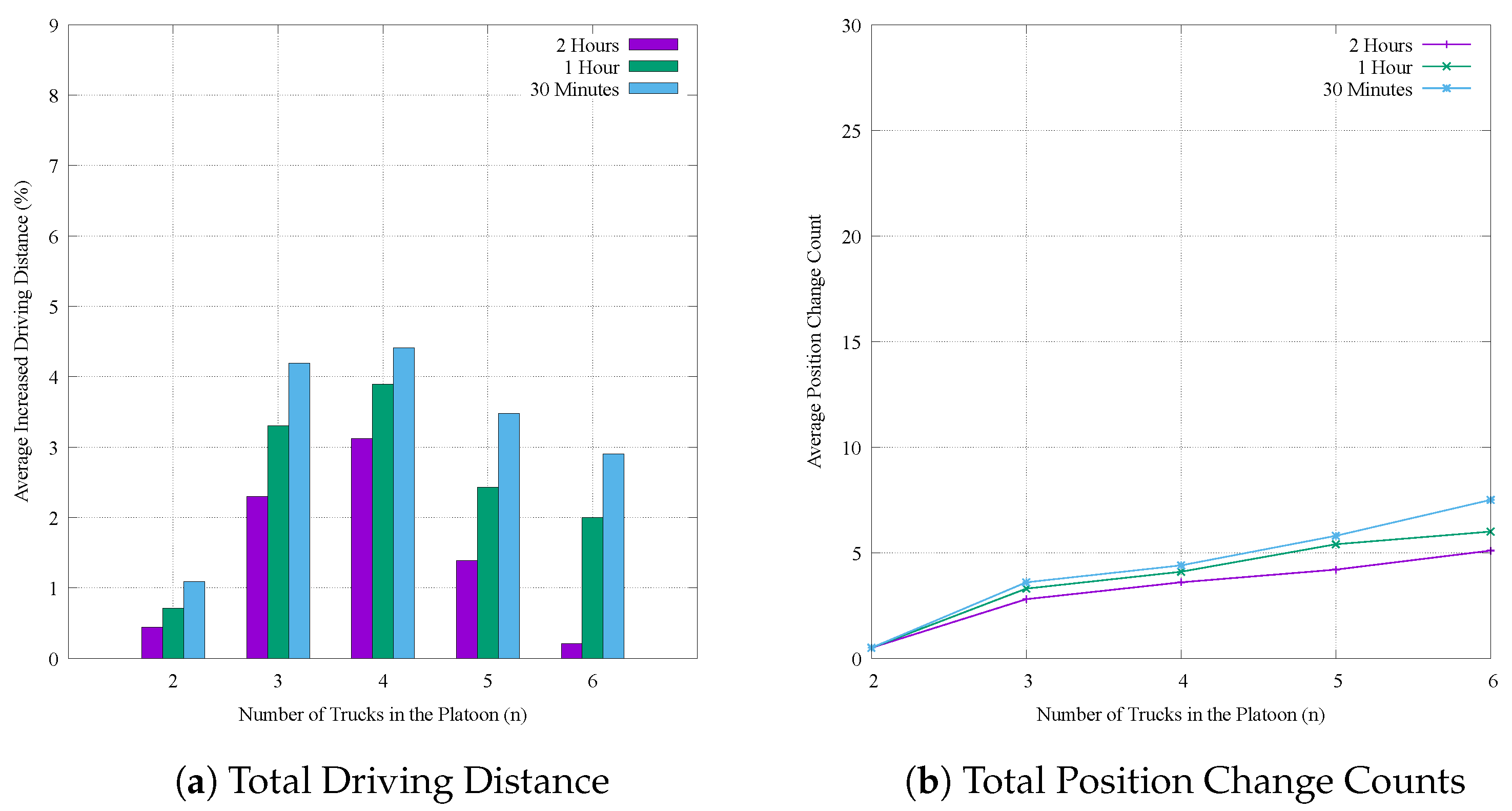
We further investigate the performance of STS when the amounts of initial fuels are unequal. We uniformly randomly select the initial fuel amount of a truck from $[250,300]$ gallons, or $[946.35,1135.62]$ L. The value of $\delta$ are set to be “30 Minutes”, “1 Hour” and “2 Hours” as in previous simulations. We run the STS algorithm ten times and calculate the averages of total distance and position change count over $n=2$ to 6. Figure 5a shows the average increased driving distance in percentage compared to the fixed order truck platooning with unequal initial fuel of 10-time runs on simulation per each $\delta$. Similar to Figure 1, the increased driving distance reaches up to 4.5%. Figure 5b presents the average position change count, where it can be seen that STS also successfully reduces position counts in the unequal initial amount of fuel. It should be noted that the distance enhancements are not as high as the case of equal initial fuel amount. This is because since the initial fuel amounts are unequal, during a number of initial time slots, the positions of the trucks may not change much. Then, the fixed order case may show similar sequences to the case of applying our algorithms. Nonetheless, we can conclude that STS successfully reduces position counts while achieving the higher driving range, regardless of the amount of initial fuel.

5. Discussion

In this section, we discuss our architectural heuristic approaches in both positive and negative details. We first discuss and compare the computation complexity of the three proposed heuristic algorithms.

In “Fuel Amount Heuristic (FAH)”, we first need to select the optimal threshold c that makes the driving distance prolonged to the maximum, yet with a reduced position change count. Since two adjacent vehicles should switch their positions when their fuel amounts are far apart from more than or equal c, the value of c should be small enough to make the position change possible, thus achieving a higher driving distance. However, it should not be too small, as it can make a large number of position change counts and waste energy for unnecessary position change operations. The computation complexity goes to the question, “What is the optimal c and how can we obtain it?”. In order to find the optimal c, we also need to look at other parameters, especially the initial fuel amount of each vehicle. We may have to conduct several rounds of trials and compare the results, which may cost high computation. The complexity goes even higher when considering the realistic scenarios of computing the actual fuel energy along traveling, not just one but all in convoy. Therefore, we recognize taking high computational cost as a negative point for FAH.

Similar to “Traveling Time Heuristic (TTH)”, the maximum increased driving distance with a small number of position change count can be obtained with the small value of $\delta$. Even though our simulation results show no remarkable difference in total driving distance, still with the small number of time slots, the possibility of position change is lower likewise. Therefore, there is no influential difficulty in choosing the value $\delta$. However, when considering the higher number of vehicles and a small amount of $\delta$ aspects, this may lead to the complicated position arrangement in a practical environment, since vehicles should align in the decreasing order in each time slot.

“Sorted Time Slot (STS)” promises a significant reduction in position change. However, remarkably, it negatively affects processing times as it has to sort vehicle position arrangement for all time slots such that it can move duplicate columns into consecutive columns after the position change heuristic algorithm is applied. Basically, the time complexity of our algorithms without STS methodology is $O(n^2\times \frac{distance}{\delta })$. With STS, the time complexity becomes $O(n^2\times \frac{distance}{\delta }\times k)$. Therefore, our STS may be inefficient on a large number of vehicles in platooning with the small value of $\delta$.

6. Conclusions and Future Works

Platooning technology benefits in reducing fuel energy consumption because a cooperative automated driving system with a small inter-vehicle helps the aerodynamic drag effect decrease. Even though the advantages of introduced fuel-saving already prolong the total driving distance of the platoon, we perceive a potential way to improve the driving range to be higher, thus enhancing fuel-saving to be the most efficient. Since vehicles at the front of the platoon will experience more air resistance than the rears, thereby consuming much more energy, vehicles in the platoon should change position from time to time so that each consumes nearly the same amount of fuel. In this paper, we propose two-position change heuristic algorithms to enhance fuel efficiency by balancing fuel consumption in each vehicle to get the highest increased driving range, “Fuel Amount Heuristic (FAH)” and “Traveling Time Heuristic (TTH)”. Furthermore, we also propose an enhancement of the original position change algorithms called “Sorted Time Slot (STS)” to decrease the number of position changes, as the higher number of changes, the more possibility of wasting fuel energy in unnecessary position change operations.

Through our demonstrated simulations, the results show that the proposed algorithm helps to increase the total driving distance significantly. The extended driving range reaches approximately 3% compared to the fixed order platooning in two-truck platooning and accomplishes around 8% increase in six-truck platooning. Therefore, we can conclude that the more vehicles in the platoon, the more driving range increases. Our improved position change algorithm (STS) also results in a reduced number of position changes by ensuring non-duplicated position arrangement along the traveling so that the number of position change counts decreases. We accomplish our purpose for truck platooning technology—to obtain the longest maximum driving distance with a fewer number of position changes, preventing more fuel loss in the process of the position change. In future works, we plan to apply our proposed algorithms to various scenarios and more realistic transportation environments to see whether those algorithms are possible to be implemented with practice-ready truck platooning.