Article

Unsupervised Anomaly Approach to Pedestrian Age Classification from Surveillance Cameras Using an Adversarial Model with Skip-Connections

by
Husnu Baris Baydargil
1,
Jangsik Park
1,* and
Ibrahim Furkan Ince
1,2
1
Department of Electronics Engineering, Kyungsung University, Busan 48434, Korea
2
Department of Digital Game Design, Nisantasi University, Maslak Mahallesi, Tasyoncasi Sokak, No: 1V, No:1Y Kod: 34481742 Sariyer, Istanbul 34398, Turkey
*
Author to whom correspondence should be addressed.
Appl. Sci. 2021, 11(21), 9904; https://doi.org/10.3390/app11219904
Submission received: 4 September 2021 / Revised: 5 October 2021 / Accepted: 12 October 2021 / Published: 23 October 2021
(This article belongs to the Topic Applied Computer Vision and Pattern Recognition)

Abstract

:
Anomaly detection is an active research area within the machine learning and scene understanding fields. Despite the ambiguous definition, anomaly detection is considered an outlier detection in a given data based on normality constraints. The biggest problem in real-world anomaly detection applications is the high bias of the available data due to the class imbalance, meaning a limited amount of all possible anomalous and normal samples, thus making supervised learning model use difficult. This paper introduces an unsupervised and adversarially trained anomaly model with a unique encoder–decoder structure to address this issue. The proposed model distinguishes different age groups of people—namely child, adult, and elderly—from surveillance camera data in Busan, Republic of Korea. The proposed model has three major parts: a parallel-pipeline encoder with a conventional convolutional neural network and a dilated-convolutional neural network. The latent space vectors created at the end of both networks are concatenated. While the convolutional pipeline extracts local features, the dilated convolutional pipeline extracts the global features from the same input image. Concatenation of these features is sent as the input into the decoder, which has partial skip-connection elements from both pipelines. This, along with the concatenated feature vector, improves feature diversity. The input image is reconstructed from the feature vector through the stacked transpose convolution layers. Afterward, both the original input image and the corresponding reconstructed image are sent into the discriminator and are distinguished as real or fake. The image reconstruction loss and its corresponding latent space loss are considered for the training of the model and the adversarial Wasserstein loss. Only normal-designated class images are used during the training. The hypothesis is that if the model is trained with normal class images, then during the inference, the construction loss will be minimal. On the other hand, if the untrained anomalous class images are input through the model, the reconstruction loss value will be very high. This method is applied to distinguish different age clusters of people using unsupervised training. The proposed model outperforms the benchmark models in both the qualitative and the quantitative measurements.

1. Introduction

Anomaly detection is an essential study field in visual image understanding. It is defined as an unexpected pattern recognition that is significantly different from the rest of the data. Some of the significant challenges include imbalanced data distribution, the difficulty of a generalizable feature extractor, variance in anomaly situations, and various environmental conditions in the data. There has been a massive surge in the availability of publicly available real-world datasets following recent trends. However, in most of these datasets, the class imbalance towards normal classes and lack of abnormal classes means these datasets lack diversity and are not capable of efficiently training supervised detection models [1]. In addition, labeling the data is a labor-intensive and costly endeavor. Deep learning models require large amounts of data for optimal performance, and the developed systems may have only a limited utility and sub-optimal generalization [2]. Under such cases, unsupervised anomaly detection has become the standard approach to such data distribution modeling. In such scenarios, the model is trained only with normal-designated class images to capture the data distribution. Afterward, the inference is performed with both normal and abnormal images to detect the deviation from the learned distribution of the normal data.
Various approaches have been proposed [3,4,5] for different domains for anomaly detection [6,7,8]. It is generally assumed that abnormal cases differ in higher and lower dimensional space, making the latent space a vital part of anomaly detection. Recent studies propose generative adversarial networks (GANs) [9] for anomaly detection due to their efficient mapping of the data distribution of both high-dimensional and low-dimensional features [10].
Public space is defined as a place that is open and accessible to people, including roads, public squares, parks, and beaches. Creating safer public spaces requires actions such as enhancing the security level against public security threats. Unemployment and different pathologies usually cause crime and economic inequality [11]. An increase in the population also increases this threat caused by anonymity and weaker interpersonal ties [12]. It is crucial to reduce the rate of urban crime to make these public spaces safer, mainly focusing on the "crime triangle"—place, victim, and the perpetrator [13]. The location can also have effects on impeding the crime or facilitating it.
Video surveillance cameras have become a prominent part of public spaces. Surveillance cameras are given an increased allocated budget all over the world. For example, three-quarters of the Home Office budget was allocated to surveillance-related projects from 1996 to 1998 in Great Britain [14]. In the last decade, cities in the United States have also done substantial development projects using surveillance data, 87% for areas with 250,000 or more [15].
Violence against children is defined as all forms of violence against people under 18. This act may come from parents, caregivers, peers, or strangers. It includes physical, sexual, and emotional violence as well as witnessing the violence. An estimated 1 billion children have experienced any form of violence aged 2–17 years [16]. This indicates that population-based surveillance of violence against the most vulnerable of the society, the children, and ordinary people is essential to target prevention and is endorsed in the United Nations 2030 Sustainable Development Agenda.
In this paper, an unsupervised anomaly detection model for different age groups of people, namely child, adults, and elderly, is proposed to achieve this goal. The proposed model has a parallel pipeline feature extractor, a conventional cascading convolutional neural network (CNN), and a cascading dilated convolutional neural network (DCN) with a dilation rate of two. At the end of both pipelines, the extracted features in the shape of fully connected layers are concatenated and then become the input for the generator, where it is used to reconstruct the original input image. The generator has partial-skip connections in a UNet-fashion [17] from both the CNN and the DCN pipeline, which allows the information from the shallow layers to propagate more efficiently to deeper layers [18] to alleviate the vanishing gradient problem, and the mode collapse [19]. Afterward, both the input image and the reconstructed output image are sent to a discriminator to be distinguished as real or fake. The discriminator’s latent vector also learns the reconstructed normal input’s latent space in the proposed scheme. The motivation to combine two sub-networks comes from the dilated convolution’s capability to extract global features without increasing the computational cost [20,21], and the combination of both the local and the global features improves the performance of the model as it was previously applied in the field of machine learning by concatenating the extracted local and global features which are then subsequently trained with traditional machine learning classifiers such as SVM [22,23]. In other words, the proposed scheme applies the same philosophy into a deep learning model by having both sub-networks extract these features automatically and then concatenate them as a result of the training. Moreover, as a part of the ablation study of the parallel encoder, supervised training is performed with a Softmax layer with three nodes added to the end of the concatenated feature vector to perform supervised classification.
To sum up, in this paper, an unsupervised anomaly detection model for age classes (child, adult, elderly) using surveillance image data is introduced. There are no unsupervised anomaly detection models for age detection with only full-body images to the authors’ best knowledge. The majority of the models are supervised and are based on facial features [24]. The deep learning model proposed in this paper is the extended and improved version of the previous work introduced in [25]. The multi-class normality scheme is applied where a single class in the dataset is designated to be the abnormal class, and the remaining classes are designated to be the normal class. The proposed model performs better than the authors’ previous work and all the benchmark models qualitatively and quantitatively.

2. Related Work

Starting with AlexNet’s [26] superior performance in The ImageNet Large Scale Visual Recognition Challenge (ILSVRC) against conventional methods, deep learning models have also created a new spark of interest in anomaly detection. With broad real-world applicable areas such as video surveillance [5], and biomedical engineering [4], a large number of papers have been published using anomaly detection [27]. The proposed model in this paper also follows recent reconstruction-based trends.
An influential model proposed by Schlegl et al. [4] uses adversarial training. In the paper, it is hypothesized that the latent vector of the GAN represents the data distribution. However, the authors initially train a generator and a discriminator with only normal images to achieve this. Afterward, using the frozen weights of the pre-trained generator and discriminator, they remap to the latent vector by optimizing the model based on its latent vector. The model shows an anomaly by showing a high anomaly score during the testing, a significantly better score than previous works. The main drawback of this proposal is the computational complexity due to the two-stage approach, and latent vector remapping is computationally costly. Following this work, Zenati et al. [28] use BiGAN [29], applying joint training to map the data distribution from the image and the latent space. Akcay et al. [10] propose an autoencoder (GANomaly) with an additional encoder added to the decoder’s end to train this autoencoder and the discriminator jointly. Afterward, Akcay et al. [30] propose an additional anomaly detection model with skip-connections trained jointly with the discriminator.
Human age in the literature is generally classified into four major categories: child (0–12 years), adolescent (13–18), adult (19–59), and senior adult (60 and above) [31]. Most of the age group classification approaches are either gait-based [31] or focus facial features [32]. These approaches range from using support vector machines [33] to complex CNN architectures [34]. However, the major issue with these approaches is that the choice of the dataset is labeled. These approaches have minimal use for real-time surveillance usage. External conditions such as lighting, image quality, positioning of the pedestrians, occlusion through other people, and other objects often cause less-than-ideal scenarios. The proposed model is trained to distinguish the abnormal and normal images and jointly minimize the distance between their latent vector representations.
As reconstruction-based approaches [4,10,28,30] show promising results in anomaly detection; a solution to this problem is the proposed unsupervised anomaly detection approach, where the input data does not have a label. Surveillance camera footage captured from regions in the Republic of Korea is used to train the proposed model. The pedestrians observed in the surveillance cameras are selectively cropped and are manually labeled with age classes, namely, the child, adult, and elderly. A total of 80% of the normal classes in a cluster to learn the data distribution of these classes is used for training. For comparison, the remaining 20% of the normal class images and an equal amount of corresponding anomalous class images are input through the model. An anomaly score is obtained for each image. The abnormal image’s deviation from the normal distribution is shown in its anomaly score compared with normal images, and this is used to detect outlier cases.

3. Proposed Model

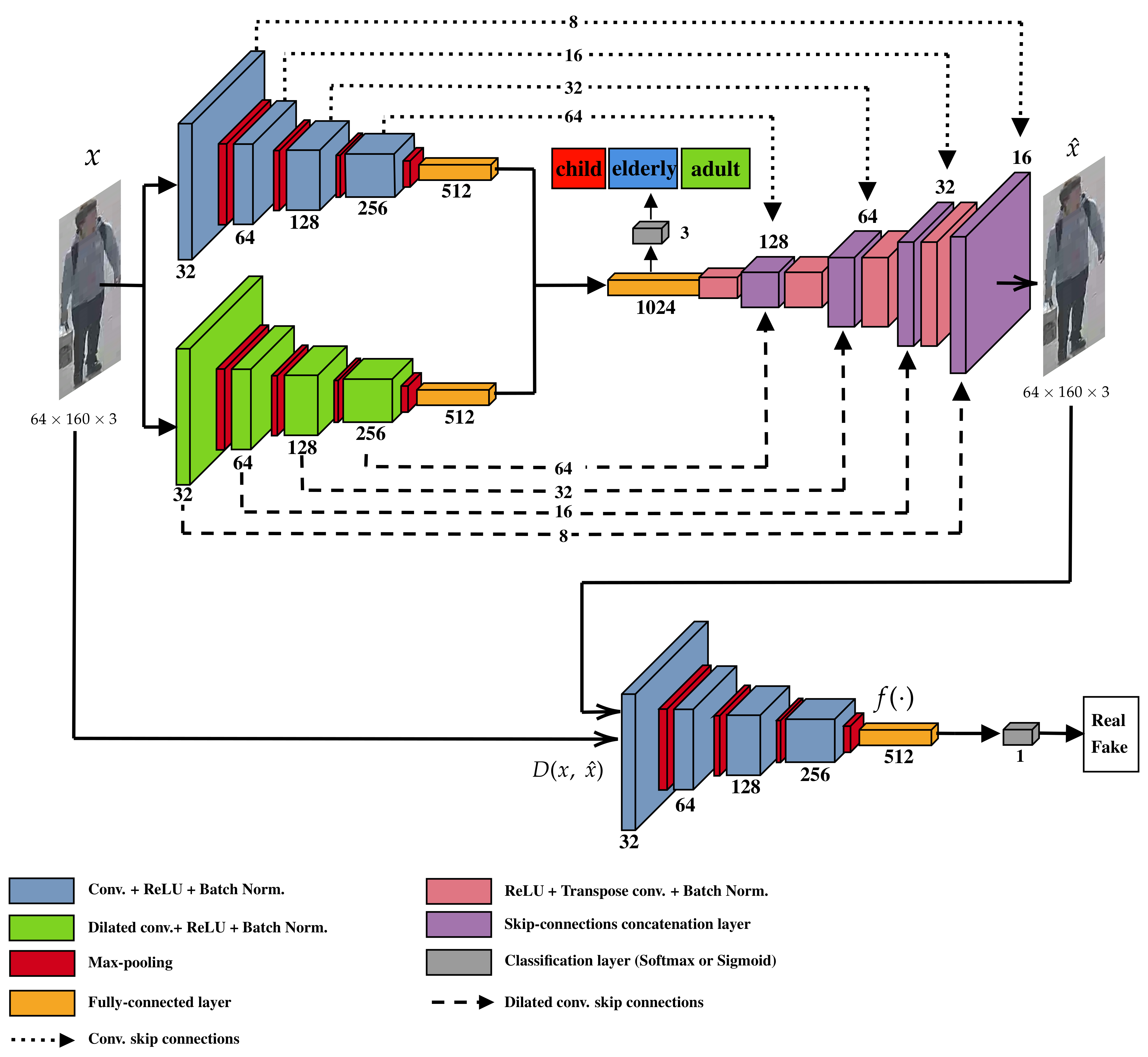
The proposed model is built with two primary components: the generator (G) and the discriminator (D) as shown in Figure 1. The generator includes an encoder with two cascading parallel sub-networks, a conventional convolutional pipeline (CNN), and a dilated convolutional pipeline (DCN) with a dilation factor of two. Both pipelines are four layers deep. Each layer uses 3 × 3 convolutional filters, followed by a rectified linear unit (ReLU) activation function, a batch normalization operation [35], and a max-pooling operation for spatial dimension reduction. This also means that the computational cost is identical between both the CNN and DCN (dilation rate has no effect on the computational complexity). The reasoning behind the parallel DCN is that the dilated convolutions increase the receptive field of the network while keeping the number of coefficients the same as its conventional counterpart, causing it to capture more global features [36]. The latent space vector created by the concatenation of the features obtained from CNN and DCN becomes the input of the decoder part of the generator. The four layer-deep up-sampling layers also concatenate the skip-connections from CNN and DCN to enable multi-scale capturing of the image space with high capability [37]. In the scenario of replacing the DCN with a CNN with 5 × 5 convolutions, the computational cost would increase 2.78 times due to the massive increase in the number of trainable parameters (from 387,840 trainable parameters to 1,077,334 trainable parameters). Moreover, 3 × 3 convolutions are highly optimized for modern computing libraries on GPU and CPU. Winograd algorithm [38] which is designed specifically for 3 × 3 convolutions with stride 1, is well supported by libraries like cuDNN [39].
The generator reconstructs a corresponding image x ^ from the input image x such that G : x z where x R ( w × h × c ) and z R d . The input image is sent through both CNN and DCN, and at the end of each network, the feature vectors are concatenated into the latent space vector z.
The discriminator (D) is comprised of a four-layer cascading CNN that is responsible for predicting the correct class (i.e., real or fake) based on the features of the input image. Its structure is identical to the CNN sub-network in the generator, with 3 × 3 convolutional filters, ReLU activation, and a batch normalization operation. At the end of the fully connected layer, there is a prediction layer that classifies normal images x and corresponding reconstructed images x ^ . When adversarially trained, the discriminator improves its capability to predict until the convergence is reached. A Softmax layer is also added at the end of the concatenated feature vector as an individual classification layer as an ablation study of the model. In this ablation study, the parallel feature extracting encoder is trained in a supervised method with the labeled dataset.
The dataset is split into the training set D t r containing N normal images where D t r = { x 1 , , x N } , and a test set D t e of A normal and abnormal images combined D t e = { ( x ^ 1 , y 1 ) , , { x ^ A , y A } where y A [ 0 , 1 ] denoting normal and abnormal classes, respectively. The main task is to train the model f on D t r and perform inference on D t e . In an ideal scenario, the size of the training set should be much larger than the testing set. Training helps the model map the dataset distribution in all vector spaces, causing it to learn both higher and lower-level features distinctly different from abnormal samples.
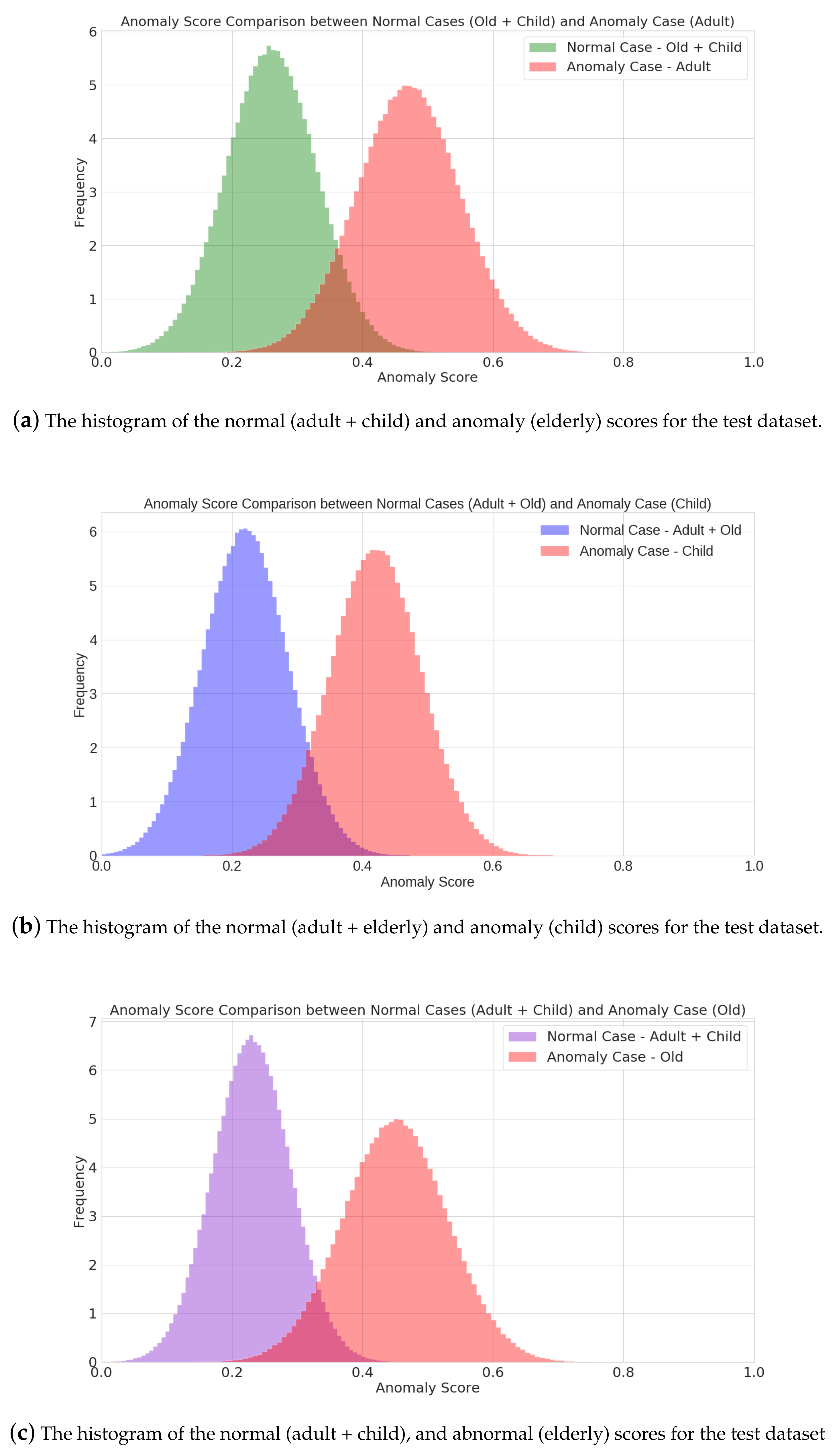
The task of the training is to capture and map the distribution of the training set D t r in both the image space and the latent vector space. It is hypothesized that defining an anomaly score A ( . ) should yield minimal scores for normal samples used in training but higher scores for abnormal samples that the model is not trained with. A higher anomaly score A ( x ) would indicate the sample x is from an abnormal class with respect to the data distribution learned by f from D t r .
Three loss functions have been implemented to train the proposed model. Each of the loss functions has its weighting in the training objective.
  • Contextual Loss: L 1 normalization between the input image x and the corresponding reconstructed image x ^ is applied to learn the image distribution. This causes the model to generate contextually similar images from normal samples. The loss is defined as:
    L c o n t e x t = E x p x | x x ^ | 1 .
  • Adversarial Loss: Wasserstein loss proposed in [40] is applied to improve the reconstruction performance for normal image x during training. This loss is helpful for the generator to reconstruct an image x ^ from the input image x as realistic as possible while helping the discriminator to classify real or fake (generated) samples. It is defined as:
    W ( q , p ) = min D max D D E x P r [ D ( x ) ] E x ^ P g [ D ( x ^ ) ]
    where D is the set of 1-Lipshitz functions and P g is the model distribution defined by x ^ = G ( z ) , z P ( z ) . The discriminator in WGAN is sometimes called a critic since it is not explicitly trained to classify; it minimizes the value function with respect to the generator parameters, W ( P r , P g ) .
  • Latent Loss: The L 2 loss is used to reconstruct the latent representations for the input x and the corresponding reconstruction x ^ . This ensures the network is sufficiently trained to produce contextually meaningful latent representations for normal samples. The final feature vector layer of the discriminator is used to obtain the features of the input image z = f ( x ) and for the reconstructed image, z ^ = f ( x ^ ) . The loss becomes:
    L l a t e n t = E x p x | f ( x ) f ( x ^ ) | 2 .
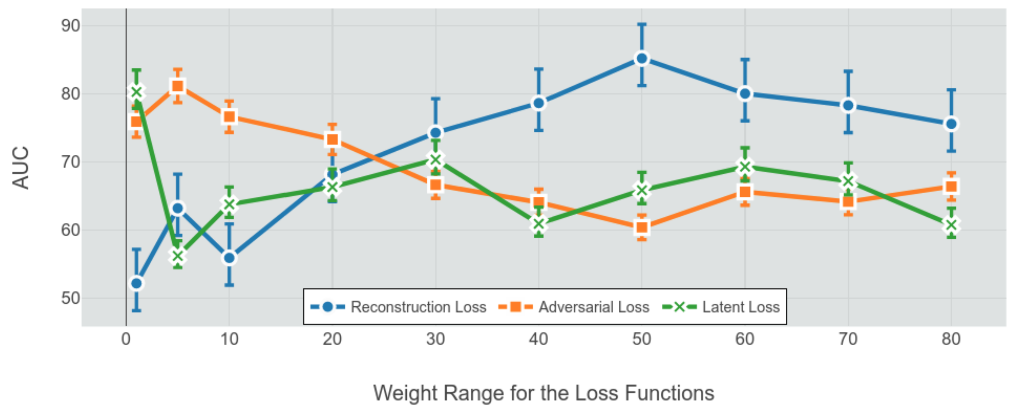
The total loss for the model becomes the weighted sum of all the losses:
L t o t a l = λ c o n t e x t L c o n t e x t + λ a d v L a d v + λ l a t e n t L l a t e n t .
where λ is the weighting parameter to assign the importance of individual losses. The optimal weighting in this study is done via a grid search operation. The optimal values for the weights can be seen in Figure 2.

4. Experimental Environment and Results

4.1. The Dataset

The dataset is obtained from various surveillance footage in the city of Busan Citizen’s Park, the Republic of Korea, with the permission of the Electronics and Telecommunication Research Institute (ETRI). Conventionally placed surveillance cameras (on top of metal poles) capture multiple areas. The full-body profile of each person is visible without undesired high-angle views. Furthermore, a ground-truth tool is made to crop and extract the pedestrians from multiple images. All of the images in the dataset have the same external conditions, such as lighting and the time of day. The total number of images in the dataset and the class-specific numbers can be seen in Table 1. The dataset split is arranged for multi-class normality, where a single class in the dataset is chosen to be the anomaly, and the rest of the classes are assigned as the normal class.
Only full-body images without any occlusion or truncation are used to generate the dataset. However, the distance of pedestrians in raw images from surveillance cameras varies significantly due to their relative position against the camera; the smallest image has 24 × 38 × 3 resolution (farthest pedestrian), and the largest image having 278 × 432 × 3 (closest pedestrian). These images are resized to the arithmetic mean resolution found in the dataset, which is found to be 64 × 160 × 3 . A set of example images in the dataset can be seen in Figure 3. The dataset is split between the anomaly cluster and normal cluster for each specific case, which are child anomaly vs. adult + elderly normal, adult anomaly vs. child + elderly normal, and elderly anomaly vs. child + elderly normal. During the training phase, the model is only trained with 80% of the normal-designated class. The remaining 20% of the normal-designated class and the anomaly class with an equal number of images are used during the testing phase. For instance, the proposed model is initially trained with 80% of the adult + elderly. The remaining 20% of images and the equal number of images from the anomalous class, child, are used for the inference. The detailed information about the train-test split can be found in Table 2.

4.2. Model Training

Modern anomaly detection models such as Skip-GANomaly [30], and AnoGAN [4] train the model on the majority of the normal-designated dataset and then run inference on the remaining normal data along with the unseen anomaly data. As a result, normal sample images are expected to have a low reconstruction loss, and their latent vectors will have similar characteristics. However, abnormal sample images are expected to fail in both cases since these images are from a class with which the model has not been trained.
Root Mean Square Propagation (RMSProp) optimization function with γ = 0.9 , η = 0.001 parameters are used for the model training. Three separate loss functions with specific weighting, shown in Section 3, are applied. Optimal loss weighting is found to be λ c o n t e x t = 50 , λ l a t e n t = 1 , λ a d v = 5 after a grid search shown in Figure 2. Model is trained for 50 epochs until the convergence was achieved. The batch size is taken as 128. Implementation of the system is done using TensorFlow [41] (Python 3.6.9, CUDA 10.0, cuDNN 7.3). The training is done on two NVIDIA P5000 GPUs. The anomaly score introduced in [29] gives a proper indication that the input image is considered real or fake, which is given in Equation (5) below:
A ( x ^ ) = ( 1 λ ) · R ( x ^ ) + λ · L ( x ^ )
where R ( x ^ ) is the reconstruction loss calculating the similarity between the real input image and the generated image based on Equation (1), and L ( x ^ ) is the latent representation loss calculating the difference between the real input image and the reconstructed image based on Equation (3). λ is the weighting parameter of the importance of each of the functions. In this study, λ = 0.2 is employed by default.
The next step is calculating the anomaly score for each inference image x ^ in the test set D t e and assign an anomaly score A such that A = { A i : A ( x ^ ) , x D t e } . Following the method proposed in [10], feature scaling (min-max normalization) is applied to A to scale the obtained scores within the range [ 0 , 1 ] . The updated anomaly score then becomes:
A ( x ^ ) = A ( x ^ ) m i n ( A ) m a x ( A ) m i n ( A )
After obtaining the A ( x ^ ) , for the entire test set, the obtained vectors are used to plot the anomaly score shown in Figure 4.

4.3. Experimental Results

The initial performance test of the proposed model, the ablation study, and the benchmark models (previously proposed anomaly detection model [25], Skip-GANomaly [30], GANomaly [10], EGBAD [28], and AnoGAN [4] is done by calculating the area under the curve (AUC) of the receiver operating characteristics (ROC). AUC is a function created using true-positive rates (TPR) and false-positive rates (FPR) with different threshold values during the inference process. The results for all the models can be seen in Table 3.
A qualitative evaluation metric called Frechet Inception Distance (FID) [42] is calculated for the proposed model and the benchmark models. This method is designed to evaluate the generated image quality by calculating the distance of feature vectors between the real image and the corresponding reconstructed image. This estimation is done using the Inception-v3 [43] image classification model. The conditional class probability and the confidence score of each image are combined. This is shown as:
F I D = | μ r μ g | 2 + T r ( r + g 2 ( r r g ) 1 / 2 )
where X r N ( μ r , r ) and X g N ( μ g , g ) are 2048-dimensional final average pooling activations (which is the default layer selected in this study) for real input images and the corresponding generated images. If both images are identical, the score should be 0. Although a lower score means better performance, an acceptable value for unsupervised learning is generally not known. In this study, a total of 500 constructed images from all three classes (adult, child, and elderly) are compared with their real counterparts, and an average FID score for all classes is obtained. The FID score comparison between the proposed model and the benchmark models can be seen in Table 4.
The third performance metric used for inference is classification accuracy. To achieve this, the parallel encoder network using both the CNN and the DCN has a Softmax layer (three nodes representing the three classes), added to the end of its feature vector, and supervised training is performed. For this training, stochastic gradient descent (SGD) with lambda decay and Nesterov momentum with the initial learning rate 10 2 is used for the proposed model and the benchmark models. Both the proposed model and the benchmark models are trained for 40 epochs. The benchmark models such as DenseNet-169 [44], Inception-v4 [45], ResNet-101 [46], and VGG19 [47] are compared with the proposed model’s classification accuracy. The classification results can be seen in Table 5.
To investigate the superior classification accuracy of the parallel feature extractor, different methods are investigated. One of the ways to explain this phenomenon is by investigating the class activation maps of the trained model during the inference. The following steps are taken during the inference:
  • Test data images are input into the parallel model, and the activation maps from each layer of sub-networks and the parallel model are obtained separately.
  • Probability density function (PDF) of each activation map is calculated, and the mean PDF is generated for both the CNN, DCN, and the parallel model.
  • Entropy is calculated from the average PDF for three separate modules (CNN, DCN, and the parallel model).
Entropy is considered a measure of randomness or uncertainty in an image, meaning the higher the entropy, the more complex the unpredictability [48]. According to Table 6, the parallel model has the lowest entropy for three classes, followed by the CNN and followed by the DCN. These values directly correspond to the corresponding model’s classification performance of the specific class.
Anomaly score comparison between three cases (normal-elderly vs. anomaly-child + adult, normal-child vs. anomaly-adult+elderly, normal-adult vs. anomaly-child+elderly) can be seen in Figure 4. Looking at the difference between the distributions between the normal and the abnormal cases, the proposed model is highly capable of distinguishing during the single-class anomaly detection inference.

5. Conclusions

In this study, an unsupervised, encoder-decoder model that is adversarially trained with skip-connections for age classification from CCTV data is proposed. The CNN sub-network of the proposed model extracts local features, and the DCN sub-network extracts global features of the input image. The potency of the parallel model is explained through the ablation study of the entropy images of sub-networks. The Latent vectors of these sub-networks are concatenated and become the input of the decoder, where the input image is reconstructed through transpose convolution. Both CNN and DCN networks have skip connections with the decoder-counterpart, assisting in the vanishing gradient problem. Afterward, the reconstructed image and the input image are input into the discriminator, where they are classified as real or fake. In the unsupervised training scheme, the model is trained with only normal-designated classes without labels. During the inference, the normal-designated classes and the anomaly-designated class is sent through the model, and the AUC and anomaly scores are calculated. The proposed model achieves up to 5% higher AUC score, 2% higher classification accuracy when fine-tuned, and an average of 1.568 lower FID score for three classes (child, adult, and elderly) than the next-best benchmark model. For future works, various methods for improving the proposed deep learning model will be investigated.

Author Contributions

Conceptualization, H.B.B. and J.P.; methodology, H.B.B. and J.P.; software, H.B.B.; validation, J.P. and I.F.I.; formal analysis, H.B.B., J.P., and I.F.I.; investigation, H.B.B., J.P., and I.F.I.; resources, J.P.; data curation, H.B.B.; writing—original draft preparation, H.B.B.; writing—review and editing, H.B.B. and J.P.; visualization, H.B.B.; supervision, J.P. and I.F.I.; project administration, J.P.; funding acquisition, J.P. All authors have read and agreed to the published version of the manuscript.

Funding

This research was supported by the BB21 plus funded by Busan Metropolitan City and Busan Institute for Talent & Lifelong Education (BIT) and Special Research Fund 2020 of Kyungsung University.

Institutional Review Board Statement

The study was conducted according to the guidelines of the Declaration of Helsinki and approved by the Institutional Review Board of Kyungsung University.

Informed Consent Statement

The surveillance dataset was obtained from the Electronics and Telecommunications Research Institute (ETRI), which is a South Korean government-funded research institute. Therefore, the subject consent used in the research was waived.

Data Availability Statement

The raw dataset was obtained from the Electronics and Telecommunications Research Institute (ETRI), South Korea. Due to the privacy laws regarding the protection of the recorded individuals with the surveillance cameras, the dataset used in this study is not publicly available.

Acknowledgments

The surveillance data used in this experiment was obtained from the Electronics and Telecommunications Research Institute (ETRI), South Korea.

Conflicts of Interest

The authors declare no conflict of interest. The funders had no role in the design of the study; in the collection, analyses, or interpretation of data; in the writing of the manuscript, or in the decision to publish the results.

Abbreviations

The following abbreviations are used in this manuscript:
CNNConvolutional Neural Network
DCNDilated Convolutional Neural Network
DCGANDeep Convolutional Generative Adversarial Networks
AnoGANAnomaly GAN
EGBADEfficient GAN-Based Anomaly Detection
BiGANBidirectional GAN
ReLURectified Linear Units
GANsGenerative Adversarial Networks
AUCArea Under the Curve
FIDFrechet Inception Distance
SGDStochastic Gradient Descent
RMSPropRoot Mean Square Propagation

References

  1. Johnson, J.M.; Khoshgoftaar, T.M. Deep Learning and Data Sampling with Imbalanced Big Data. In Proceedings of the 2019 IEEE 20th International Conference on Information Reuse and Integration for Data Science (IRI), Los Angeles, CA, USA, 30 July–1 August 2019; pp. 175–183. [Google Scholar] [CrossRef]
  2. Willemink, M.J.; Koszek, W.A.; Hardell, C.; Wu, J.; Fleischmann, D.; Harvey, H.; Folio, L.R.; Summers, R.M.; Rubin, D.L.; Lungren, M.P. Preparing Medical Imaging Data for Machine Learning. Radiology 2020, 295, 4–15. [Google Scholar] [CrossRef] [PubMed]
  3. Ahmed, M.; Naser Mahmood, A.; Hu, J. A survey of network anomaly detection techniques. J. Netw. Comput. Appl. 2016, 60, 19–31. [Google Scholar] [CrossRef]
  4. Schlegl, T.; Seeböck, P.; Waldstein, S.M.; Schmidt-Erfurth, U.; Langs, G. Unsupervised Anomaly Detection with Generative Adversarial Networks to Guide Marker Discovery. arXiv 2017, arXiv:cs.CV/1703.05921. [Google Scholar]
  5. Kiran, B.R.; Thomas, D.M.; Parakkal, R. An Overview of Deep Learning Based Methods for Unsupervised and Semi-Supervised Anomaly Detection in Videos. J. Imaging 2018, 4, 36. [Google Scholar] [CrossRef] [Green Version]
  6. Hodge, V.; Austin, J. A Survey of Outlier Detection Methodologies. Artif. Intell. Rev. 2004, 22, 85–126. [Google Scholar] [CrossRef] [Green Version]
  7. Pimentel, M.A.; Clifton, D.A.; Clifton, L.; Tarassenko, L. A review of novelty detection. Signal Process. 2014, 99, 215–249. [Google Scholar] [CrossRef]
  8. Chandola, V.; Banerjee, A.; Kumar, V. Anomaly Detection: A Survey. ACM Comput. Surv. 2009, 41. [Google Scholar] [CrossRef]
  9. Goodfellow, I.J.; Pouget-Abadie, J.; Mirza, M.; Xu, B.; Warde-Farley, D.; Ozair, S.; Courville, A.; Bengio, Y. Generative Adversarial Nets. In Proceedings of the 27th International Conference on Neural Information Processing Systems, NIPS’14, Montreal, QC, Canada, 8–13 December 2014; MIT Press: Cambridge, MA, USA, 2014; Volume 2, pp. 2672–2680. [Google Scholar]
  10. Akcay, S.; Atapour-Abarghouei, A.; Breckon, T.P. GANomaly: Semi-Supervised Anomaly Detection via Adversarial Training. arXiv 2018, arXiv:cs.CV/1805.06725. [Google Scholar]
  11. Horwitz, A.V. The Economy and Social Pathology. Annu. Rev. Sociol. 1984, 10, 95–119. [Google Scholar] [CrossRef]
  12. Granovetter, M. The Strength of Weak Ties. Am. J. Soc. 1973, 6, 1360–1380. [Google Scholar] [CrossRef] [Green Version]
  13. Tillyer, M.; Eck, J. Getting a handle on crime: A further extension of routine activities theory. Secur. J. 2010. [Google Scholar] [CrossRef]
  14. Armitage, R. To CCTV or Not to CCTV?: A Review of Current Research into the Effectiveness of CCTV Systems in Reducing Crime. 2002. Nacro Crime and Social Policy Section 237 Queenstown Road London SW8 3NP. Available online: http://eprints.hud.ac.uk/id/eprint/2542/ (accessed on 13 October 2021).
  15. Reaves, B.A. Local Police Departments, 2013: Equipment and Technology; U.S. Department of Justice, Office of Justice Programs, Bureau of Justice Statistics: Washington, DC, USA, 2015; NCJ 248767; Available online: https://bjs.ojp.gov/library/publications/local-police-departments-2013-equipment-and-technology (accessed on 21 June 2021).
  16. Hillis, S.; Mercy, J.; Amobi, A.; Kress, H. Global Prevalence of Past-year Violence Against Children: A Systematic Review and Minimum Estimates. Pediatrics 2016, 137. [Google Scholar] [CrossRef] [Green Version]
  17. Ronneberger, O. U-Net: Convolutional Networks for Biomedical Image Segmentation. arXiv 2015, arXiv:abs/1505.04597. [Google Scholar]
  18. Drozdzal, M.; Vorontsov, E.; Chartrand, G.; Kadoury, S.; Pal, C. The Importance of Skip Connections in Biomedical Image Segmentation. arXiv 2016, arXiv:cs.CV/1608.04117. [Google Scholar]
  19. Yang, Y.; Jin, R.; Xu, C. On the Effects of Skip Connections in Deep Generative Adversarial Models. In Proceedings of the Fourth International Conference On Computer Science And Artificial Intelligence, Zhuhai, China, 11–13 December 2020; 57, p. 57. [Google Scholar] [CrossRef]
  20. Lin, Y.; Wu, J. A Novel Multichannel Dilated Convolution Neural Network for Human Activity Recognition. Math. Probl. Eng. 2020, 2020. [Google Scholar] [CrossRef]
  21. Chim, S.; Lee, J.G.; Park, H.H. Dilated Skip Convolution for Facial Landmark Detection. Sensors 2019, 19, 5350. [Google Scholar] [CrossRef] [Green Version]
  22. Lisin, D.; Mattar, M.; Blaschko, M.; Learned-Miller, E.; Benfield, M. Combining Local and Global Image Features for Object Class Recognition. In Proceedings of the 2005 IEEE Computer Society Conference on Computer Vision and Pattern Recognition (CVPR’05)—Workshops, San Diego, CA, USA, 21–23 September 2005; p. 47. [Google Scholar] [CrossRef] [Green Version]
  23. Kabbai, L.; Abdellaoui, M.; Douik, A. Image classification by combining local and global features. Vis. Comput. 2018, 35, 679–693. [Google Scholar] [CrossRef]
  24. Horng, W.B.; Lee, C.P.; Chen, C.W. Classification of Age Groups Based on Facial Features. Tamkang J. Sci. Eng. 2001, 4, 183–192. [Google Scholar]
  25. Baydargil, H.B.; Park, J.S.; Kang, D.Y. Anomaly Analysis of Alzheimer’s Disease in PET Images Using an Unsupervised Adversarial Deep Learning Model. Appl. Sci. 2021, 11, 2187. [Google Scholar] [CrossRef]
  26. Krizhevsky, A.; Sutskever, I.; Hinton, G.E. ImageNet Classification with Deep Convolutional Neural Networks. Commun. ACM 2017, 60, 84–90. [Google Scholar] [CrossRef]
  27. Markou, M.; Singh, S. Novelty detection: A review-part 1: Statistical approaches. Signal Process. 2003, 83, 2481–2497. [Google Scholar] [CrossRef]
  28. Zenati, H.; Foo, C.S.; Lecouat, B.; Manek, G.; Chandrasekhar, V.R. Efficient GAN-Based Anomaly Detection. arXiv 2019, arXiv:cs.LG/1802.06222. [Google Scholar]
  29. Donahue, J.; Krähenbühl, P.; Darrell, T. Adversarial Feature Learning. arXiv 2017, arXiv:1605.09782. [Google Scholar]
  30. Akcay, S.; Atapour Abarghouei, A.; Breckon, T. Skip-GANomaly: Skip Connected and Adversarially Trained Encoder-Decoder Anomaly Detection. In Proceedings of the 2019 International Joint Conference on Neural Networks (IJCNN), Budapest, Hungary, 14–19 July 2019; pp. 1–8. [Google Scholar] [CrossRef] [Green Version]
  31. Li, X.; Makihara, Y.; Xu, C.; Yagi, Y.; Ren, M. Gait-Based Human Age Estimation Using Age Group-Dependent Manifold Learning and Regression. Multimed. Tools Appl. 2018, 77, 28333–28354. [Google Scholar] [CrossRef] [Green Version]
  32. Liu, X.; Zou, Y.; Kuang, H.; Ma, X. Face Image Age Estimation Based on Data Augmentation and Lightweight Convolutional Neural Network. Symmetry 2020, 12, 146. [Google Scholar] [CrossRef] [Green Version]
  33. Cortes, C.; Vapnik, V. Support-vector networks. Chem. Biol. Drug Des. 2009, 297, 273–297. [Google Scholar] [CrossRef]
  34. Dehghan, A.; Ortiz, E.; Shu, G.; Masood, S.Z. DAGER: Deep Age, Gender and Emotion Recognition Using Convolutional Neural Network. arXiv 2017, arXiv:cs.CV/1702.04280. [Google Scholar]
  35. Ioffe, S.; Szegedy, C. Batch Normalization: Accelerating Deep Network Training by Reducing Internal Covariate Shift. arXiv 2015, arXiv:cs.LG/1502.03167. [Google Scholar]
  36. Baydargil, H.B.; Park, J.; Kang, D.Y.; Kang, H.; Cho, K. A Parallel Deep Convolutional Neural Network for Alzheimer’s disease classification on PET/CT brain images. KSII Trans. Internet Inf. Syst. 2020, 14. [Google Scholar] [CrossRef]
  37. Schuster, R.; Wasenmuller, O.; Unger, C.; Stricker, D. SDC-Stacked Dilated Convolution: A Unified Descriptor Network for Dense Matching Tasks. In Proceedings of the 2019 IEEE/CVF Conference on Computer Vision and Pattern Recognition (CVPR), Long Beach, CA, USA, 15–20 June 2019; pp. 2551–2560. [Google Scholar] [CrossRef] [Green Version]
  38. Lavin, A.; Gray, S. Fast Algorithms for Convolutional Neural Networks. In Proceedings of the 2016 IEEE/CVF Conference on Computer Vision and Pattern Recognition (CVPR), Las Vegas, NV, USA, 27–30 July 2016; pp. 4013–4021. [Google Scholar]
  39. Chetlur, S.; Woolley, C.; Vandermersch, P.; Cohen, J.; Catanzaro, B.; Shelhamer, E. cuDNN: Efficient Primitives for Deep Learning. arXiv 2014, arXiv:1410.0759. [Google Scholar]
  40. Arjovsky, M.; Chintala, S.; Bottou, L. Wasserstein Generative Adversarial Networks. In Proceedings of the 34th International Conference on Machine Learning, Sydney, NSW, Australia, 6–11 August 2017; Volume 70, pp. 214–223. [Google Scholar]
  41. Abadi, M.; Agarwal, A.; Barham, P.; Brevdo, E.; Chen, Z.; Citro, C.; Corrado, G.S.; Davis, A.; Dean, J.; Devin, M.; et al. TensorFlow: Large-Scale Machine Learning on Heterogeneous Systems. 2015. Available online: tensorflow.org (accessed on 12 July 2021).
  42. Heusel, M.; Ramsauer, H.; Unterthiner, T.; Nessler, B.; Hochreiter, S. GANs Trained by a Two Time-Scale Update Rule Converge to a Local Nash Equilibrium. In Proceedings of the 31st International Conference on Neural Information Processing Systems, Long Beach, CA, USA, 4–9 December 2017; Curran Associates Inc.: Red Hook, NY, USA, 2017; pp. 6629–6640. [Google Scholar]
  43. Szegedy, C.; Vanhoucke, V.; Ioffe, S.; Shlens, J.; Wojna, Z. Rethinking the Inception Architecture for Computer Vision. In Proceedings of the 2016 IEEE Conference on Computer Vision and Pattern Recognition (CVPR), Las Vegas, NV, USA, 27–30 June 2016; IEEE Computer Society: Los Alamitos, CA, USA, 2016; pp. 2818–2826. [Google Scholar] [CrossRef] [Green Version]
  44. Huang, G.; Liu, Z.; Van Der Maaten, L.; Weinberger, K.Q. Densely Connected Convolutional Networks. In Proceedings of the 2017 IEEE Conference on Computer Vision and Pattern Recognition (CVPR), Honolulu, HI, USA, 21–26 July 2017; pp. 2261–2269. [Google Scholar] [CrossRef] [Green Version]
  45. Szegedy, C.; Ioffe, S.; Vanhoucke, V.; Alemi, A.A. Inception-v4, Inception-ResNet and the Impact of Residual Connections on Learning. In Proceedings of the Thirty-First AAAI Conference on Artificial Intelligence, San Francisco, CA, USA, 4–9 February 2017; AAAI Press: Palo Alto, CA, USA, 2017; pp. 4278–4284. [Google Scholar]
  46. He, K.; Zhang, X.; Ren, S.; Sun, J. Deep Residual Learning for Image Recognition. In Proceedings of the 2016 IEEE Conference on Computer Vision and Pattern Recognition (CVPR), Las Vegas, NV, USA, 26 June–1 July 2016; pp. 770–778. [Google Scholar] [CrossRef] [Green Version]
  47. Simonyan, K.; Zisserman, A. Very Deep Convolutional Networks for Large-Scale Image Recognition. arXiv 2015, arXiv:cs.CV/1409.1556. [Google Scholar]
  48. Thum, C. Measurement of the Entropy of an Image with Application to Image Focusing. Opt. Acta: Int. J. Opt. 1984, 31, 203–211. [Google Scholar] [CrossRef]
Figure 1. The proposed model architecture. The input image x size is 64 × 160 × 3 for both the encoder and the discriminator D ( x , x ^ ) . Encoder architecture has two sub-networks: a conventional CNN and a dilated convolutional CNN (DCN). Both CNN and DCN have 3 × 3 convolutional layers, with DCN having a dilation factor of two. At the end of both networks, the latent vectors are concatenated and become the input of the generator where the input image x is reconstructed as x ^ through the transpose convolution layers. In addition, a Softmax layer is added to this latent vector for the ablation test. When the parallel encoder is trained with the labeled data, classification is performed in this layer. Partial skip-connections from CNN and DCN into the generator model alleviate the vanishing gradient and the mode collapse phenomenons observed in deep learning models. Afterward, both the input image and the reconstructed images are sent through the discriminator. The images are classified as either real or fake in the sigmoid layer (with one node). The fully connected layer of the discriminator f ( · ) is utilized for anomaly detection during the inference. Each input image, whether it belongs to a normal-designated class or an anomaly-designated class, results in a reconstruction score, based on Equation (6).
Applsci 11 09904 g001
Figure 2. Loss function range search results for reconstruction loss, adversarial loss, and the latent loss. The model shows optimal performance with the parameters λ c o n t e x t = 50 , λ a d v = 5 , and λ l a t e n t = 1 . The most important weighting parameter is found to be the λ c o n t e x t .
Applsci 11 09904 g002
Figure 3. Example images from each class in the dataset: (a) Adult class, (b) Child class, and (c) Elderly class. It should be noted that in each class, there are also images of pedestrians moving in different directions (front-facing, back-facing, side-facing) and with different lighting conditions. Variation in the distance of pedestrians against the camera causes many images to have less-than-ideal quality, which should be taken into consideration in real-life applications.
Applsci 11 09904 g003
Figure 4. Anomaly scores for three different cases. The normalization of the anomaly value for each image of the test dataset forms a normal distribution in the histogram. It is expected that the normal inference images will form a normal distribution closer to zero, and the abnormal inference images will form a normal distribution closer to one.
Applsci 11 09904 g004
Table 1. The dataset information about the total number of images for each class.
ClassesNumber of Images
Elderly2809
Adult4477
Child1922
Total9208
Table 2. The train-test split of the dataset. A total of 80% of two normal-designated class images are used in a cluster during the training without labels, and the remaining 20% of each normal-designated class, as well as the equal-numbered anomaly-designated class images, are used during the inference. Anomaly-designated class images are not used during the training.
TrainTest
CasesAdultChildElderlyTotalAdultChildElderlyTotal
Anomaly (Child) vs. Normal (Adult + Elderly)2247-3581582856214588962916
Anomaly (Adult) vs. Normal (Child + Elderly)-15373581511812813858962562
Anomaly (Elderly) vs. Normal (Adult + Child)22471537-37845623859471894
Table 3. The results for the area under the curve (AUC) of receiver operating characteristics (ROC) of the proposed model, the previously proposed model for Alzheimer’s disease anomaly detection, the ablation study of the single convolutional pipeline as well as the single dilated convolutional pipeline, Skip-GANomaly, GANomaly, EGBAD, and AnoGAN.
NormalAnomalyProposed ModelConv. OnlyD. Conv. OnlyPrevious Model [25]Skip-GANomaly [30]GANomaly [10]EGBAD [28]AnoGAN [4]
Adult + ElderlyChild88.4582.3675.8485.0783.3480.4579.6378.57
Child + AdultElderly83.4381.6673.0180.4479.3278.8276.1674.53
Child + ElderlyAdult84.1680.7271.5882.8981.2580.0175.3473.42
Table 4. FID score comparison for three different classes (Adult, Child, and Elderly) for the benchmark models, the proposed model, and the ablation study of the proposed model. Note that a lower score generally means better performance.
ModelsAdultChildElderly
EGBAD [28]20.33421.51019.817
AnoGAN [4]19.43920.14518.056
GANomaly [10]15.31016.48114.006
Skip-GANomaly [30]8.3659.9316.480
Previous Model [25]6.9427.4186.569
Ablation Conv.8.62110.0156.714
Ablation Dilated Conv.13.14814.21011.729
Proposed Model5.1286.3324.765
Table 5. The classification accuracy results for the proposed model, the ablation study (convolutional pipeline-only, and dilated convolutional pipeline-only), and the benchmark classification models including DenseNet-169, Inception-v4, ResNet-101, and VGG19.
ClassesFull ModelConv. OnlyD. Conv. OnlyDenseNet-169 [44]Inception-v4 [45]ResNet-101 [46]VGG19 [47]
Adult89.9183.3478.3887.4686.5183.4582.20
Elderly90.2481.5276.2387.9082.4381.9880.71
Child86.8084.2777.5684.5380.9280.2678.43
Table 6. Entropy values of the class activation maps (CAMs) from CNN and DCN modules and the parallel model. The entropy values and the classification accuracy have a correlation on classification accuracy, caused by the unpredictability, which can be seen in Table 5.
ClassesCNNDCNParallel Model
Adult2.437822.823461.61425
Elderly2.372592.905231.59523
Child2.502242.912931.63562
Publisher’s Note: MDPI stays neutral with regard to jurisdictional claims in published maps and institutional affiliations.

